The Influence of Quantum Critical Fluctuations of Circulating Current Order Parameters on the Normal State Properties of Cuprates

Abstract

We study a model of the quantum critical point of cuprates associated with the ”circulating current” order parameter proposed by Varma. An effective action of the order parameter in the quantum disordered phase is derived using functional integral method, and the physical properties of the normal state are studied based on the action. The results derived within the ladder approximation indicate that the system is like Fermi liquid near the quantum critical point and in disordered regime up to minor corrections. This implies that the suggested marginal Fermi liquid behavior induced by the circulating current fluctuations will come in from beyond the ladder diagrams.

I Introduction

In spite of the intensive studies of the last 15 years the microscopic origin of the high temperature superconductors (HTSC) still remains elusive. However, the physical properties in each regime of phase diagram are now well established. [1] The normal state properties of the cuprate supercondcutors are highly anomalous. They deviate substantially from the Fermi liquid behavior and are believed to be of a non-Fermi liquid. Especially, the anomalous normal state properties near optimal doping concentration can be characterized by the phenomenological marginal Fermi liquid (MFL) theory. [2] The MFL theory rests on a single hypothesis that there exist excitations whose spectral function is given by

$${\rm Im}P(\omega,{\bf q})\sim\cases{-N(E_{F})\frac{\omega}{T},\quad|\omega|\ll T\cr-N(E_{F}){\rm sgn}\omega,\quad|\omega|\gg T,}$$ (1)

where $N(E_{F})$ is the unrenormalized density of states at the Fermi energy, and ${\rm sgn\omega}=\omega/|\omega|$. The important features of the spectral function Eq. (1) are its independence of the momentum ${\bf q}$ and its scaling form as a function of $\omega/T$. The $\omega/T$ scaling is the hallmark of quantum critical point (QCP), thus the scaling form of the spectral function very strongly suggests a proximate QCP. If QCP indeed underlies the MFL behaviour, the momentum independence of Eq. (1) implies infinitely large dynamical exponent $z_{d}$ of QCP.

Most of the normal state properties associated with two-particle correlations near optimal doping have been found consistent with the MFL theory. [2] Recently, the validity of MFL was confirmed also for single-particle properties. The recent angle-resolved photoemission experiment by Valla et al. [3] found that the single-particle self-energy is given by the MFL form. They measured the imaginary part of the electron self-energy of the optimal Bismuth HTSC along a nodal direction, and obtained ${\rm Im}\Sigma({\bf k},\epsilon)\sim\max(|\epsilon|,T)$. This observation renewed the interest in the MFL theory, and especially, in the microscopic basis of the MFL and conjectured proximate QCP.

There are several models rooted on the idea of QCP which attempt to explain various aspects of HTSC[4, 5, 6]. In general, it is necessary to introduce a certain local order parameter to define a QCP. The present experimental data put strong constraint on the possible form of the order parameter. In particular, there is no evidence of broken translational symmetry, so the order parameter of QCP should be chosen to respect the translational symmetry. The theory by C. M. Varma [4, 5] is based on the order parameter which does respect the translation symmetry but breaks the time reversal symmetry and the four-fold rotation symmetry. The construction of such order parameter necessitates the full set of the copper $d$ and the oxygen $p_{x,y}$ orbitals. The explicit form of the (complex) order parameter is

$$\Psi(T,x)=\frac{V}{2}\sum_{{\bf p},\sigma}\langle\sin\frac{p_{x}a}{2}d^{\dagger}_{{\bf p}\sigma}p_{x{\bf p}\sigma}-\sin\frac{p_{y}a}{2}d^{\dagger}_{{\bf p}\sigma}p_{y{\bf p}\sigma}\rangle,$$ (2)

where $V$ is coupling constant, and $a,x$ is lattice constant of unit cell[7] and doping concentration, respectively. $\sigma$ is spin quantum number. At zero temperature, $\Psi(T=0,x<x_{c})\neq 0$. The critical doping $x_{c}\sim 0.2$ [5, 8] defines the QCP.

In QCP theory of HTSC by Varma, the anomalous normal state corresponds to the finite temperature region of the disordered regime $T>T_{c}>0,x\sim x_{c}$. In this regime the critical fluctuations of order parameter determine the physical properties. Varma made an extensive study on the general class of models which can give rise to the order parameter (2), and gave an heuristic (and essentially non-perturbative) derivation of the susceptibility $\chi(\omega,{\bf q})$ which controls the critical fluctuation of order parameter in the normal state[4]. In this paper, we have chosen a simplified model considered by Varma [5] and derived an effective action (See Eq.(20).) of the order parameter systematically in the functional integral formalism. Such effective action can be also regarded as time-dependent Landau-Ginzburg type free energy. The lowest order term of the effective action (See Eq.(30).) amounts to the summation of the ladder-type diagrams. The physical properties deduced from the lowest order term of the effective action are not compatible with the experimental data of the normal states. For an example, the electron self-energy derived from the lowest order effective action is Fermi liquid-like apart from logarithmic correction. If we accept the heuristic derivations by Varma, the inadequacy of the lowest order approximation implies the importance of higher order terms beyond the ladder diagrams.

This paper is organized as follows: In Sec.II, we introduce our model and derive the functional integral representation of the effective action. In Sec.III, the concrete form of the effective action is obtained up to the 4th order. In Sec.IV, we analyze the effective action following Moriya’s self-consistent renormalization scheme, and calculate some physical quantities. In Sec.V, we conclude this paper with the summary and some concluding remarks.

II Formulation

The basic model is the three-band Hubbard model[4, 5, 9].

$$H = H_{0}+H_{1}+H_{2},$$ (3)

$$H_{0} = \sum_{{\bf k},\sigma}\,\Big{(}\epsilon_{d}\,n_{d{\bf k}\sigma}+2t_{pd}d^{\dagger}_{{\bf k}\sigma}\big{[}s_{x}({\bf k})p_{x{\bf k}\sigma}+s_{y}({\bf k})p_{y{\bf k}\sigma}\big{]}-4t_{pp}s_{x}({\bf k})s_{y}({\bf k})p^{\dagger}_{x{\bf k}\sigma}p_{y{\bf k}\sigma}+{\rm H.C.}\Big{)},$$ (4)

$$H_{1} = \sum_{i\sigma}\,U_{d}n_{di\sigma}n_{di-\sigma}+U_{p}(n_{pxi\sigma}n_{pxi-\sigma}+n_{pyi\sigma}n_{pyi-\sigma}),$$ (5)

$$H_{2} = 2V\sum_{{\bf k},{\bf k}^{\prime},{\bf q},\sigma,\sigma^{\prime}}\,c_{x}({\bf q})\,d^{\dagger}_{{\bf k}+{\bf q}\sigma}d_{{\bf k}\sigma}\,p^{\dagger}_{x{\bf k}^{\prime}-{\bf q}\sigma^{\prime}}p_{x{\bf k}^{\prime}\sigma^{\prime}}+c_{y}({\bf q})\,d^{\dagger}_{{\bf k}+{\bf q}\sigma}d_{{\bf k}\sigma}\,p^{\dagger}_{y{\bf k}^{\prime}-{\bf q}\sigma^{\prime}}p_{y{\bf k}^{\prime}\sigma^{\prime}}.$$ (6)

$i$ is a lattice site index, and $c_{x,y}({\bf k})=\cos\frac{k_{x,y}a}{2},s_{x,y}({\bf k})=\sin\frac{k_{x,y}a}{2}$. $H_{1}$ is the on-site repulsion term which suppresses the doubly occupied states. $H_{2}$ is the nearest neighbor repulsion ($V>0$) term between copper $d$ and oxygen $p_{x},p_{y}$ orbitals written in momentum space. The order parameter of circulating current (CC) phase comes from $H_{2}$. To simplify our problem, we implement the effect of $H_{1}$ by a substitution $t_{pd}\to xt_{pd},\;t_{pp}\to xt_{pp}$[5]. Certainly, this is very crude approximation and the effect of $H_{1}$ shoud be more carefully included in due course.

It is easy to show, by re-indexing momenta, that $H_{2}$ can be written as

$$H_{2} = -V\sum_{i=1,2,3,4\sigma\sigma^{\prime}}\hat{O}^{\dagger}_{\sigma\sigma^{\prime}i}\hat{O}_{\sigma^{\prime}\sigma i}$$ (7)

$$\hat{O}_{1\sigma^{\prime}\sigma}({\bf q}) = \sum_{{\bf k}^{\prime}}\,\Big{(}s_{{\bf k}^{\prime}x}p^{\dagger}_{x{\bf k}^{\prime}\sigma^{\prime}}-s_{{\bf k}^{\prime}y}p^{\dagger}_{y{\bf k}^{\prime}\sigma^{\prime}}\Big{)}\,d_{{\bf k}^{\prime}+{\bf q}\sigma},$$ (8)

$$\hat{O}_{2\sigma^{\prime}\sigma}({\bf q}) = \sum_{{\bf k}^{\prime}}\,\Big{(}s_{{\bf k}^{\prime}x}p^{\dagger}_{x{\bf k}^{\prime}\sigma^{\prime}}+s_{{\bf k}^{\prime}y}p^{\dagger}_{y{\bf k}^{\prime}\sigma^{\prime}}\Big{)}\,d_{{\bf k}^{\prime}+{\bf q}\sigma},$$ (9)

$$\hat{O}_{3\sigma^{\prime}\sigma}({\bf q}) = \sum_{{\bf k}^{\prime}}\,\Big{(}c_{{\bf k}^{\prime}x}p^{\dagger}_{x{\bf k}^{\prime}\sigma^{\prime}}-c_{{\bf k}^{\prime}y}p^{\dagger}_{y{\bf k}^{\prime}\sigma^{\prime}}\Big{)}\,d_{{\bf k}^{\prime}+{\bf q}\sigma},$$ (10)

$$\hat{O}_{4\sigma^{\prime}\sigma}({\bf q}) = \sum_{{\bf k}^{\prime}}\,\Big{(}c_{{\bf k}^{\prime}x}p^{\dagger}_{x{\bf k}^{\prime}\sigma^{\prime}}+c_{{\bf k}^{\prime}y}p^{\dagger}_{y{\bf k}^{\prime}\sigma^{\prime}}\Big{)}\,d_{{\bf k}^{\prime}+{\bf q}\sigma}.$$ (11)

The expectation value of the operator $\hat{O}_{1\sigma\sigma}\equiv\hat{O}_{1\sigma}$ is the order parameter of CC phase Eq.(2) up to constant factor. Because the critical fluctuation of $\hat{O}_{1\sigma}$ is most dominant near QCP, the remainder $H_{2}^{\prime}=-V\sum_{i=2,3,4,\sigma^{\prime}\sigma}\hat{O}^{\dagger}_{\sigma^{\prime}i}\hat{O}_{\sigma i}-V\sum_{\sigma^{\prime}\neq\sigma}\hat{O}^{\dagger}_{\sigma^{\prime}\sigma 1}\hat{O}_{\sigma\sigma^{\prime}1}$ can be treated as perturbations near QCP. We will not take the effect of $H_{2}^{\prime}$ into account explicitly in this work. Note that the operator $\hat{O}_{1\sigma}$ is odd under the $C_{4}$ symmetry of square lattice. The reduced Hamiltonian which incoporates the physics associated with CC phase is

$$\tilde{H} = \sum_{{\bf k},\sigma}\,\Big{(}\epsilon_{d}\,n_{d{\bf k}\sigma}+2td^{\dagger}_{{\bf k}\sigma}\big{[}s_{x}({\bf k})p_{x{\bf k}\sigma}+s_{y}({\bf k})p_{y{\bf k}\sigma}\big{]}-4t^{\prime}s_{x}({\bf k})s_{y}({\bf k})p^{\dagger}_{x{\bf k}\sigma}p_{y{\bf k}\sigma}+{\rm H.C.}\Big{)}$$ (12)

$$- V\sum_{\sigma,{\bf q}}\hat{O}_{\sigma}^{\dagger}({\bf q})\,\hat{O}_{\sigma}({\bf q}),$$ (13)

where $t\equiv xt_{pd},t^{\prime}\equiv xt_{pp}$. We could have adopted a basis where kinetic term of the reduced Hamiltonian is diagonalized. The advantage of our choice of basis is that the coupling between order parameter and fermions is simple and that it admits the formal manipulations of functional integral method. Using Hubbard-Stranovich transformation, the partition function can be written in the functional integral form.

$$Z = \int D[\Psi_{l\sigma},\bar{\Psi}_{l\sigma^{\prime}}]\,D[N_{\sigma}]\,\exp[-S(\Psi,\bar{\Psi},N)],$$ (14)

$$S = \sum_{lm,\sigma\sigma^{\prime}}\,\sum_{i\epsilon,\epsilon^{\prime},{\bf k},{\bf k}^{\prime}}\,\bar{\Psi}_{l\sigma}(i\epsilon^{\prime},{\bf k}^{\prime})\,\Big{[}K_{0}^{-1}-VM\Big{]}\,\Psi_{m\sigma^{\prime}}(\epsilon,{\bf k})+V\sum_{\sigma}\sum_{{\bf q},\omega}N_{\sigma}^{\dagger}(i\omega,{\bf q})N_{\sigma}(i\omega,{\bf q}),$$ (15)

where the six component spinor is defined $\Psi_{l\sigma}(i\epsilon,{\bf k})=\Big{(}d_{{\bf k}\sigma},p_{x{\bf k}\sigma},p_{y{\bf k}\sigma}\Big{)}$. $l,m$ are the orbital indices. The explicit form of kernel matrix is ($\mu$ is the chemical potential.)

$$K_{0}^{-1}(i\epsilon,i\epsilon^{\prime};{\bf k},{\bf k}^{\prime};lm;\sigma\sigma^{\prime})=\delta_{\epsilon\epsilon^{\prime}}\,\delta_{\sigma\sigma^{\prime}}\delta_{{\bf k}{\bf k}^{\prime}}\pmatrix{\epsilon_{d}-i\epsilon-\mu&2ts_{x}({\bf k})&2ts_{y}({\bf k})\cr 2ts_{x}({\bf k})&-i\epsilon-\mu&-4t^{\prime}s_{x}({\bf k})s_{y}({\bf k})\cr 2ts_{y}({\bf k})&-4t^{\prime}s_{x}({\bf k})s_{y}({\bf k})&-i\epsilon-\mu}.$$ (16)

The explicit form of the matrix $M$ is ($k=(i\epsilon,{\bf k}),k^{\prime}=(i\epsilon^{\prime},{\bf k}^{\prime})$.)

$$M(k^{\prime},k;\sigma^{\prime}\sigma;lm)=\delta_{\sigma\sigma^{\prime}}\pmatrix{0&N_{k^{\prime}-k}s_{x}({\bf k})&-N_{k^{\prime}-k}s_{y}({\bf k})\cr N^{\dagger}_{k-k^{\prime}}s_{x}({\bf k}^{\prime})&0&0\cr-N^{\dagger}_{k-k^{\prime}}s_{y}({\bf k}^{\prime})&0&0}.$$ (17)

The effective action of order parameter $N_{\sigma}$ can be obtained by integrating out the electrons $\Psi_{\sigma l}$. ($q=(i\omega,{\bf q})$.)

$$S_{{\rm eff}}=V\sum_{\sigma q}N^{\dagger}_{\sigma}(q)N_{\sigma}(q)-2\,\ln{\rm Det}(K_{0}^{-1}-VM),$$ (18)

where the factor of 2 of the second term comes from the spin degeneracy. From now on the spin index of $N$ will be suppressed. By expanding the determinant of (18) the (time-dependent) Landau-Ginzburg type action can be obtained. In principle, the action (18) contains all the elements for the description of the critical properties of our model. The mean-field phase diagram can be determined by minimizing (18) with respect to $N,N^{\dagger}$. Using relation $\delta\ln\det A=\delta{\rm Tr}\ln A={\rm Tr}A^{-1}\delta A$, we get

$$N^{\dagger}(q)=-2\sum_{k,k^{\prime},a,b}\left(\frac{1}{K_{0}^{-1}-VM}\right)_{k,k^{\prime};lm}\,\frac{\delta M_{k^{\prime},k;ml}}{\delta N(q)}.$$ (19)

Eq.(19) is the mean-field equation written in matrix form. According to the mean-field solution by Varma[5], Eq.(19) has a non-trivial solution for $x<x_{c}\sim 0.2$ and $T<T_{c}(x)$ with $T_{c}(x_{c})=0$. The non-trivial mean-field solution is of the form $N=iR$, where $R$ is real. It should be noted that only the solution of this type preserves $C_{4}\times T$, where $T$ is the time reversal. Thus, we expect that the susceptibility of the imaginary component of $N$ $\langle{\rm Im}N(q){\rm Im}N(-q)\rangle$ would diverge as $q\to 0,x\to x_{c}+0^{+}$ at zero temperature, reflecting the large critical fluctuation near QCP. The susceptibility determines the critical properties near QCP. In the quantum disordered phase, the mean-field equation (19) has a trivial solution $N=0$, and we may expand the action (18) as a power series of $N$.

III Effective Action

One can show that the terms with odd powers of $N$ vanish in the expansion of the determinant of (18) by using the transformation property of $N$ under $C_{4}$ rotation. Expanding the determinant up to the 4-th order we get

$$S_{{\rm eff}} = 2V\sum_{q}N^{\dagger}(q)N(q)+\sum_{q}\,\Big{[}\Pi_{A}(q)\,N(q)N^{\dagger}(q)+\Pi_{B}(q)\,(N(q)N(-q)+N^{\dagger}(q)N^{\dagger}(-q))\Big{]}$$ (20)

$$+ \sum_{q_{i},i=1,2,3,4}\,\Big{[}\Pi_{C}(q_{i})N(q_{1})N(q_{2})N^{\dagger}(q_{3})N^{\dagger}(q_{4})+\Pi_{D}(q_{i})\,N(q_{1})N^{\dagger}(q_{2})\,(N(q_{3})N(q_{4})+N^{\dagger}(q_{3})N^{\dagger}(q_{4}))$$ (21)

$$+ \Pi_{E}(q_{i})\,(N(q_{1})N(q_{2})N(q_{3})N(q_{4})+N^{\dagger}(q_{1})N^{\dagger}(q_{2})N^{\dagger}(q_{3})N^{\dagger}(q_{4}))\Big{]}+O(N^{6},N^{8},\ldots).$$ (22)

The appropriate momentum-energy conservation rules are to be understood for the 4th order terms. The explicit expressions of the polarization functions $\Pi_{i}$ are relegated to the appendix. Since the $d,p_{x},p_{y}$ electrons are the linear combinations of the anti-bonding $a$, the bonding $b$, and the non-bonding $c$ electron operators, the polarization functions $\Pi_{i}$’s contain both intra-band ($aa$) and inter-band ($ab$ or $ac$) contributions.

For analyses later, it is convenient to decompose the order parameter $N$ into the real and imaginary components. In real space ($x=(\tau,{\bf x})$.), the decomposition is

$$N(x)=N_{1}(x)+iN_{2}(x),N^{\dagger}(x)=N_{1}(x)-iN_{2}(x).$$ (23)

In momentum-frequency space,

$$N(q)=N_{1}(q)+iN_{2}(q),N^{\dagger}(q)=N_{1}(-q)-iN_{2}(-q).$$ (24)

In terms of real components $N_{1},N_{2}$ the quadratic part of the effective action (20) can be written as

$$S_{{\rm eff}}^{(2)}=\sum_{q}\Big{[}\tilde{\pi}_{1}(q)N_{1}(q)N_{1}(-q)+\tilde{\pi}_{2}(q)N_{2}(q)N_{2}(-q)\\ +i\tilde{\pi}_{3}(q)\big{(}N_{1}(q)N_{2}(-q)-N_{1}(-q)N_{2}(q)\big{)}\Big{]},$$ (25)

where

$$\tilde{\pi}_{1}(q) = 2V+\Pi_{A}(q)+2\Pi_{B}(q),$$ (26)

$$\tilde{\pi}_{2}(q) = 2V+\Pi_{A}(q)-2\Pi_{B}(q),$$ (27)

$$\tilde{\pi}_{3}(q) = 2V+\Pi_{A}(q).$$ (28)

Using the results Eq.(B21) for $\Pi_{A}(q)$ and $\Pi_{B}(q)$, $\tilde{\pi}_{i}(q)$’s ($i=1,2,3$) can be parametrized as

$$\tilde{\pi}_{i}(i\omega,{\bf q})=\delta_{i}+a_{i}|{\bf q}|^{2}+b_{i}\omega^{2}+\frac{|\omega|}{\Gamma_{i}|{\bf q}|}-i\eta\omega,$$ (29)

where $a_{1}=a_{3},\Gamma_{1}=\Gamma_{3}$. The polarization functions $\tilde{\pi}_{i}(q)$ contain both the intra-band and the inter-band contributions. In particular, the Landau damping term which exists for $|\omega|<\Gamma_{i}|{\bf q}|$ solely stems from the intra-band contribution. The parametrizations Eq.(29) are valid for $|\omega|<\mu$ (See Appendix B.). At this point, we observe that $N_{1}(q)N_{1}(-q)$ and $N_{2}(q)N_{2}(-q)$ of Eq.(25) are even in $q$, while $(N_{1}(q)N_{2}(-q)-N_{1}(-q)N_{2}(q))$ is odd in $q$. Therefore, only the even parts of $\tilde{\pi}_{1}(q)$ and $\tilde{\pi}_{2}(q)$ and the odd part of $\tilde{\pi}_{3}(q)$ contribute to $S_{{\rm eff}}^{(2)}$.

$$S_{{\rm eff}}^{(2)}=\sum_{q}\Big{[}\pi_{1}(q)N_{1}(q)N_{1}(-q)+\pi_{2}(q)N_{2}(q)N_{2}(-q)+i\pi_{3}(q)\big{(}N_{1}(q)N_{2}(-q)-N_{1}(-q)N_{2}(q)\big{)}\Big{]},$$ (30)

$$\pi_{1}(i\omega,{\bf q}) = \delta_{1}+a_{1}|{\bf q}|^{2}+\frac{|\omega|}{\Gamma_{1}|{\bf q}|}+b_{1}\omega^{2},$$ (31)

$$\pi_{2}(i\omega,{\bf q}) = \delta_{2}+a_{2}|{\bf q}|^{2}+\frac{|\omega|}{\Gamma_{2}|{\bf q}|}+b_{2}\omega^{2},$$ (32)

$$\pi_{3}(i\omega,{\bf q}) = -i\eta\omega.$$ (33)

The propagators (or the susceptibilities) of order parameters can be read off from Eq.(30,31).

$$\langle N_{1}(q)N_{1}(-q)\rangle = \frac{\pi_{2}(q)}{\pi_{1}(q)\pi_{2}(q)-(\pi_{3}(q))^{2}},$$ (34)

$$\langle N_{2}(q)N_{2}(-q)\rangle = \frac{\pi_{1}(q)}{\pi_{1}(q)\pi_{2}(q)-(\pi_{3}(q))^{2}},$$ (35)

$$\langle N_{1}(q)N_{2}(-q)\rangle = \frac{-i\pi_{3}(q)}{\pi_{1}(q)\pi_{2}(q)-(\pi_{3}(q))^{2}}.$$ (36)

Let us define $D_{ij}(q)=\langle N_{i}(q)N_{j}(-q)\rangle$. The explicit form of the $D_{22}(i\omega,{\bf q})$ is

$$D_{22}(i\omega,{\bf q})=\Big{[}\delta_{2}+a_{2}|{\bf q}|^{2}+b_{2}\omega^{2}+\frac{|\omega|}{\Gamma_{2}|{\bf q}|}+\frac{\eta^{2}\omega^{2}}{\delta_{1}+a_{1}|{\bf q}|^{2}+b_{1}\omega^{2}+\frac{|\omega|}{\Gamma_{1}|{\bf q}|}}\Big{]}^{-1}.$$ (37)

Eq.(37) is valid within the ladder approximation (See below.). As discussed in the previous section, the critical fluctuation of $N_{2}$ is important near QCP, thus the susceptibility $D_{22}(i\omega,{\bf q})$ determines the physical properties near QCP. Obviously, $\delta_{2}$ is the parameter which controls the proximity to QCP. The precise location of QCP is determined by the condition

$$[D_{22}^{(ren)}]^{-1}(i\omega\to 0,{\bf q}\to 0)=0,$$ (38)

where $D_{22}^{(ren)}(i\omega,{\bf q})$ is the fully renormalized susceptibility which includes all of the higher order corrections. Since $\delta_{1}$ is expected to be large, we can approximate the last term of (37) as $\frac{\eta^{2}}{\delta_{1}}\omega^{2}$ and absorb it into $b_{2}$. Then, within ladder approximation, the imaginary part of the retarded $D_{22}^{R}(\omega,{\bf q})$ becomes

$${\rm Im}D_{22}^{R}(\omega>0,{\bf q}) \approx \Theta(\Gamma_{2}|{\bf q}|-\omega)\frac{\frac{\omega}{\Gamma_{2}|{\bf q}|}}{(\delta_{2}+a_{2}|{\bf q}|^{2})^{2}+(\frac{\omega}{\Gamma_{2}|{\bf q}|})^{2}}$$ (39)

$$+ \Theta(\omega-\Gamma_{2}|{\bf q}|)\delta(\delta_{2}+a_{2}|{\bf q}|^{2}-b_{2}\omega^{2}),$$ (40)

where $\Theta(x)$ is the step function ($\Theta(x)=1,x>0;\Theta(x)=0,x<0$.).

If we neglect the higher order terms like $N^{4},N^{6},\ldots$, the quadratic action Eq.(30) amounts to the ladder approximation. This can be verified by the direct calculation of susceptibility $\langle\hat{O}(q)\hat{O}^{\dagger}(q)\rangle$ (See Eq.(7).) both by the functional integral formalism and the conventional perturbation theory. Then, following Mahan’s treatment of excitons [10], we might expect the excition-like poles in the susceptibility. This pole can be identified in Eq.(37) by analytic continuation $i\omega\to\omega+i\delta$. QCP in the ladder approximation is equivalent to the vanishing of the exciton-like gap.

The coefficients of the 4th order terms $\Pi_{C}(q_{i}),\Pi_{D}(q_{i}),\Pi_{E}(q_{i})$ depend on the momenta of order parameters. For small $q_{i}$’s, $\Pi_{C}(q_{i}),\Pi_{D}(q_{i}),\Pi_{E}(q_{i})$ can be expanded in $q_{i}$. Neglecting the dependences on momenta, the 4th order terms of the effective action can be expressed as (in real space $x=(\tau,{\bf x})$.)

$$S_{{\rm eff}}^{(4)}=\int d^{3}x\Big{[}\frac{\lambda_{1}}{4!}\,N_{1}^{4}(x)+\frac{\lambda_{2}}{4!}\,N_{2}^{4}(x)+\frac{\lambda_{3}}{2!2!}\,N_{1}^{2}(x)N_{2}^{2}(x)\Big{]},$$ (41)

where

$$\lambda_{1}=4!(\Pi_{C}(0)+2\Pi_{D}(0)+2\Pi_{E}(0)),\;\;\lambda_{2}=4!(\Pi_{C}(0)-2\Pi_{D}(0)+2\Pi_{E}(0)),\;\;\lambda_{3}=2!2!(2\Pi_{C}(0)-12\Pi_{E}(0)).$$ (42)

$S_{{\rm eff}}^{(4)}$ introduces the lowest order corrections beyond ladder diagrams. It also renormalizes the electron self-energy at one loop order. The importances of still higher order terms will be discussed at Sec.V.

Near QCP $\delta_{2}=0$, the naive perturbation theory breaks down because of the infrared divergences as can be demonstrated by caculating the correction to free energy with $S=S_{{\rm eff}}^{(2)}+S_{{\rm eff}}^{(4)}$. These divergences can be handled by the self-consistent renormalization scheme developed by Moriya[11].

IV Self-Consistent Renormalization

To cure the infrared divergences we have to determine the critical parameter $\delta_{2}$ self-consistently including the effect of the 4th order terms Eq.(41). The self-consistent equation in real space for the renormalized $\delta_{2}^{R}(T)$ is [11, 12]

$$\delta_{2}^{R}(T)=\delta_{2}+\frac{\lambda_{2}}{4}D_{22}(0;\delta_{1},\delta_{2}^{R}(T))+\frac{\lambda_{3}}{4}D_{11}(0;\delta_{1},\delta_{2}^{R}(T)),$$ (43)

where the dependences on the critical parameter are indicated explicitly. We can neglect the renormalization of $\delta_{1}$ since it does not control the critical behaviour. Let $\delta_{1}^{*},\delta_{2}^{*}$ be the bare value of $\delta_{1},\delta_{2}$ for which $\delta_{2}^{R}(T=0)=0$. In other words, $\delta_{1}^{*},\delta_{2}^{*}$ defines the zero temperature QCP. Then, the temperature dependence of the $\delta_{2}^{R}(T)$ for $\delta_{1}^{*},\delta_{2}^{*}$ can be determined. By subtracting the Eq.(43) at $T\neq 0$ and $T=0$ for $\delta_{1}^{*},\delta_{2}^{*}$, we get

$$\delta_{2}^{R}(T)=\frac{\lambda_{2}}{4}\Big{(}D_{22}(0;\delta_{1}^{*},\delta_{2}^{R}(T))-D_{22}(0;\delta_{1}^{*},\delta_{2}^{R}=0)\Big{)}+\frac{\lambda_{3}}{4}\Big{(}D_{11}(0;\delta_{1}^{*},\delta_{2}^{R}(T))-D_{11}(0;\delta_{1}^{*},\delta_{2}^{R}=0)\Big{)}.$$ (44)

Using the relation,

$$D_{ij}(0)=\int\frac{d^{2}{\bf q}}{(2\pi)^{2}}\int_{0}^{\infty}\frac{d\omega}{\pi}\coth\frac{\omega}{2T}{\rm Im}D_{ij}^{R}(\omega,{\bf q}).$$ (45)

we can reexpress Eq.(44) as

$$\delta_{2}^{R}(T) = \frac{\lambda_{2}}{4}\int\frac{d^{2}{\bf q}}{(2\pi)^{2}}\int_{0}^{\infty}\frac{d\omega}{2\pi}\Big{[}(\coth\frac{\omega}{2T}-1){\rm Im}D^{R}_{22,\delta_{2}^{R}(T)}(\omega,{\bf q})$$ (46)

$$+ \Big{(}{\rm Im}D^{R}_{22,\delta_{2}^{R}(T)}(\omega,{\bf q})-{\rm Im}D^{R}_{22,\delta_{2}^{R}(T)=0}(\omega,{\bf q})\Big{)}\Big{]}$$ (47)

$$+ \frac{\lambda_{3}}{4}\Big{[}D_{22}\to D_{11}\Big{]}.$$ (48)

The first term of Eq.(46) determines the temperature dependence. The last term of Eq.(46) ($D_{11}$ part ) gives the subleading contribution proportional to $T^{3}$, while the first term and the second term give $T\ln(\delta_{2}^{R}(T)+T^{2})+{\rm const.}\times\delta_{2}^{R}(T)$. At low temperature, the dominant contribution to the integral comes from the low frequency region, where the Landau damping gives the largest contribution to ${\rm Im}D^{R}(\omega,{\bf q})$. Carrying out integrals up to logarithmic accuracy, we get

$$\delta_{2}^{R}(T)\sim T\ln\frac{1}{T}.$$ (49)

Now we compute some physical properties based on the self-consistent renormalization scheme.

Specific Heat- The singular behaviour of specific heat near QCP can be obtained by computing free energy with renormalized $\delta_{2}^{R}(T)$. Integrating out order parameter $N$ with the effective action Eq. (30), we get the singular piece of the free energy in (self-consistent) ladder approximation.

$$\Delta F=\int\frac{d^{2}{\bf q}}{(2\pi)^{2}}\int_{0}^{\infty}\frac{d\omega}{\pi}\coth\frac{\omega}{2T}{\rm Im}\ln\Big{[}\pi_{1}^{R}(\omega,{\bf q})\pi_{2}^{R}(\omega,{\bf q})-(\pi_{3}^{R}(\omega,{\bf q}))^{2}\Big{]}.$$ (50)

The most dominant contribution to the free energy at low temperature comes from the low-$\omega$ region. In that region, we can neglect the $\omega^{2}$ terms of polarization functions $\pi^{R}_{i}$ in the free energy compared to Landau damping term. Then, the most singular contribution comes from $\pi_{2}^{R}(\omega,{\bf q})$.

$$\Delta F_{{\rm sing}}\sim\int\frac{d^{2}{\bf q}}{(2\pi)^{2}}\int_{0}^{\infty}\frac{d\omega}{2\pi}\coth\frac{\omega}{2T}{\rm tan}^{-1}\left(\frac{\omega/\Gamma_{2}|{\bf q}|}{\delta_{2}^{R}(T)+a_{2}|{\bf q}|^{2}}\right),$$ (51)

Using the expansion $\tan^{-1}y\sim y-y^{3}/3$, and taking derivative of $\Delta F_{{\rm sing}}$ with respect to temperature we get the singular part of the specific heat.

$$C_{v}\sim\frac{T}{\sqrt{\delta_{2}^{R}(T)}}-\frac{T^{3}}{T(\delta_{2}^{R}(T))^{3}}.$$ (52)

The above result is not compatible with experimental data in normal state which shows almost T-linear behaviour. We have to keep in mind that the result Eq.(52) is essentially due to the intra-band contribution to the polarization function $\pi_{2}^{R}$. In three dimension, the above result would be

$$C_{v}\sim T\ln\delta_{2}^{R}(T)-\frac{T^{3}}{(\delta_{2}^{R}(T))^{3}}\ln\frac{T}{\sqrt{\delta_{2}^{R}(T)}}.$$ (53)

Electron Self-Energy-The coupling between order parameter and the anti-bonding electron (conduction electron) can be obtained by substituting Eq.(A6) into Eq.(14).

$$-Va^{\dagger}_{k^{\prime}}\,\Big{[}N_{1}(k^{\prime}-k)f(k,k^{\prime})+iN_{2}(k^{\prime}-k)g(k,k^{\prime})\Big{]}\,a_{k},$$ (54)

where the coupling matrix elements are(notations are defined in Appendix A.)

$$f/g=\frac{2t}{(\xi_{A})_{k}(\xi_{A})_{k^{\prime}}}\,\Big{[}E_{A}({\bf k}^{\prime})(s_{x}^{2}({\bf k})-s_{y}^{2}({\bf k}))\pm E_{A}({\bf k})(s_{x}^{2}({\bf k}^{\prime})-s_{y}^{2}({\bf k}^{\prime}))\Big{]}.$$ (55)

Note that when the momentum transfer ${\bf k}^{\prime}-{\bf k}$ is small the matrix element $g(k,k^{\prime})$ is proportional to $({\bf k}-{\bf k}^{\prime})\cdot({\bf k}+{\bf k}^{\prime})$, therefore, the coupling with the critical order parameter $N_{2}$ is suppressed for the forward scatterings. Considering the scattering with $N_{2}$, the imaginary part of the electron self-energy can be written as

$${\rm Im}\Sigma^{R}(\epsilon,{\bf p}) = V^{2}\int\frac{d^{2}{\bf q}}{(2\pi)^{2}}\int_{0}^{\infty}\frac{d\omega}{\pi}[({\bf p}+\frac{{\bf q}}{2})\cdot{\bf q}]^{2}{\rm Im}D^{R}_{22}(\omega,{\bf q})$$ (56)

$$\times \Big{[}\delta(\epsilon+\omega-\xi^{A}_{{\bf p}+{\bf q}})(n_{B}(\omega)+n_{F}(\epsilon+\omega))+\delta(\epsilon-\omega-\xi^{A}_{{\bf p}+{\bf q}})(1+n_{B}(\omega)-n_{F}(\epsilon-\omega))\Big{]},$$ (57)

where the unimportant factors of the couplings are omitted. At zero temperature ($\delta_{2}^{R}=0$), the self-energy (56) becomes (assuming $\epsilon>0$),

$${\rm Im}\Sigma^{R}(\epsilon,{\bf p})=V^{2}\int\frac{d^{2}{\bf q}}{(2\pi)^{2}}\int_{0}^{\epsilon}\frac{d\omega}{\pi}[({\bf p}+\frac{{\bf q}}{2})\cdot{\bf q}]^{2}{\rm Im}D^{R}_{22}(\omega,{\bf q};\delta^{R}_{2}=0)\delta(\epsilon-\omega-\xi^{A}_{{\bf p}+{\bf q}}).$$ (58)

Let us first consider the zero temperature case. ${\rm Im}D^{R}_{22}(\omega,{\bf q};\delta^{R}_{2}=0)$ behave differently depending on the relative magnitude of $\omega$ and $\Gamma_{2}|{\bf q}|$ (see Eq.(39).). If $\omega>\Gamma_{2}|{\bf q}|$, then the typical values of momentum and frequency are given by $\omega\sim q_{\parallel}\sim q_{\perp}$. $q_{\parallel/\perp}$ is the component of ${\bf q}$ parallel/perpendicular to ${\bf p}$. Therefore, the $|{\bf q}|^{2}$ term in the vertex can be neglected compared to ${\bf p}\cdot{\bf q}$. Carrying out the integrals, we find the self-energy is proportional to $\epsilon^{2}$. If $\omega<\Gamma_{2}|{\bf q}|$, $\omega\sim q_{\parallel}$, while $q_{\perp}\sim\omega^{1/3}$. Therefore, $q_{\perp}\gg q_{\parallel}$, the ${\bf p}\cdot{\bf q}$ term in the vertex can be neglected compared to $|{\bf q}|^{2}$. Carrying out integrals, with the momentum cut-off of the order of the external momenta ${\bf p}$, we find the self-energy is proportional to $-\epsilon^{2}\ln\epsilon^{1/3}$. The contribution from the region $|\omega|<\Gamma|{\bf q}|$ is larger than that of from $|\omega|>\Gamma|{\bf q}|$ by a logarithmic factor. Thus, the self-energy at zero temperature is

$${\rm Im}\Sigma^{R}(\epsilon,{\bf p},T=0)\sim-\epsilon^{2}\ln|\epsilon|^{1/3}.$$ (59)

Because the vertex $[({\bf p}+\frac{{\bf q}}{2})\cdot{\bf q}]^{2}$ suppresse the low momentum processes very strongly, the self-energy does not show anomalous behaviour except for the logarithmic factor. At finite temperature, the bose factor $n_{B}(\omega)$ dominates the integral. Therefore, the frequency integral is effectively cut off by the temperature. Carrying out the integrals, we find the result is proportional to $-T^{2}\ln T^{1/3}$. Combining the results for the zero temperature and the finite temperature cases, we can write

$${\rm Im}\Sigma^{R}(\epsilon,{\bf p},T)\sim-(\max(\epsilon,T))^{2}\ln[\max(\epsilon,T)]^{1/3}.$$ (60)

The self-energy Eq.(60) is like that of Fermi-liquid apart from the minor logarithmic factor. Eq.(60) is also essentially determined by intra-band contribution to the polarization function like specific heat.

The results obtained within self-consistent renormalizaton Eq.(52, 60) are not compatible with those of MFL theory. Clearly, we have to incorporate the higher order corrections beyond ladder approximation. However, the results Eq.(52, 60) might be applicable to overdoped region, namely the deep in the disordered phase, where the critical fluctuation is less important, so that the higher order correction is not important. In this region, the temperature dependence of $\delta_{2}^{R}(T)$ can be ignored, and the results Eq.(52, 60) are consistent with the experimental data in overdoped region.

V Summary and Concluding Remarks

In summary, we have studied a model of HTSC proposed by C. M. Varma which predicts QCP associated with the circulating current order parameter. The results derived with the ladder approximation indicates that the system is like Fermi liquid near the quantum critical point and in the disordered regime. In particular, the imaginary part of electron self-energy is proportional to $[\max(\epsilon,T)]^{2}$ up to minor logarithmic correction. Thus, the ladder approximation is not sufficient in describing the properties anomalous normal state, for which MFL theory gives adequate phenomenological description. For the proper explanation of the anomalous normal state properties the consideration of higher order corrections beyond ladder approximation seems to be crucial.

To get some clues on the role of higer order correction, let us estimate a higher order digram which corresponds to the vertex correction of the susceptibility $D_{22}(i\omega,{\bf q})$ beyond ladder approximation. Let us consider the renormalization of the susceptibility by the 4th order terms of (20). The full momentum and frequency dependences of $\Pi_{C}(q_{i}),\Pi_{D}(q_{i}),\Pi_{E}(q_{i})$ should be retained in evaluating the higher order correction. As has been discussed in Sec.IV, the coupling between the anti-bonding conduction electrons and the order parameter is strongly suppressed for small momentum transfer. As can be shown directly by substituting (A6) into (14) and (17), the coupling $a^{\dagger}_{{\bf p}+{\bf q}}b_{\bf p}N_{2}({\bf q})+{\rm H.C.}$ is not suppressed at small ${\bf q}$. Thus, we have to consider a diagram which renormalize $D_{22}$ with only ($a^{\dagger}_{{\bf p}+{\bf q}}b_{\bf p}N_{2}({\bf q})+{\rm H.C.}$)-type vertex. The first of such diagram is (See Fig.1),

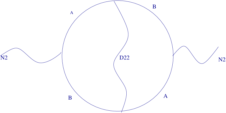
FIG. 1.: A higher order diagram which renormalize the susceptibility $\langle N_{2}N_{2}\rangle$. The roman letter A, B indicates the Green function $G_{A/B}$ (see Eq.(A7).), and the wiggly line is the propagator $D_{22}(k)$.

With the notations $q=(i\omega,{\bf q}),p=(i\epsilon,{\bf p}),k=(i\Omega,{\bf k})$, the analytic expression of Fig. 1 is

$$({\rm Fig.1})\sim V^{4}\sum_{p,k}\,G_{B}(p)G_{A}(p+k)G_{B}(p+k+q)G_{A}(p+q)D_{22}(k),$$ (61)

where the non-singular parts of vertices are omitted. The most singular contribution coming from the low energy region can be estimated as follows: First, put $k=0$ in $G_{A/B}$ and do $p$ integral. Second, carry out the remaining integral in $k$. If any infrared divergence occurs, cut the divergence by $\max(q,\delta_{2})$. The result of $p$ integral is

$$I_{p}\sim\frac{1}{\omega^{2}}\,\ln\Big{[}1+\frac{\omega^{2}}{(E_{B}(k_{F})-\mu)^{2}}\Big{]}.$$ (62)

Major contribution in momentum integral comes from $|{\bf p}|>p_{F}$, where ${\bf q}$ can be neglected. Usually $\omega^{2}\ll(E_{B}(k_{F})-\mu)^{2}$, then $I_{p}$ is non-singular. The diagram Fig.1 gives non-singular contribution, which just renormalizes some coefficients of the susceptibility. Therefore, the straightforward perturbative computation at two loop order does not give indications of singular behaviour. However, if we assume, following Varma’s heuristic derivation [4], that in the strong coupling limit (large $V$) $E_{B}(k_{F})-\mu$ can be replaced by an excitonic energy scale which corresponds $\delta_{2}$ in our notation, then $I_{p}$ becomes highly singular as we approach the quantum critical point $(\delta_{2}\rightarrow 0)$. The justification of the above replacement and the further investigation of consequences of the singularity will be further studied. The approach using the (non-perturbative) dynamical mean-field theory[13] is currently under investigation.

ACKNOWLEDGEMENTS

We are grateful to Chandra Varma for useful discussions and comments on the manuscript. We are also thankful to Yunkyu Bang for discussions on the three-band Hubbard models. This work was supported by the Korea Science and Engineering Foundation (KOSEF) through the grant No. 1999-2-11400-005-5, and by the Ministry of Education through Brain Korea 21 SNU-SKKU Program.

A Diagonalization of Kinetic Term

The fermion Green functions can be obtained by inverting the kernel matrix $K_{0}^{-1}$ Eq.(16). The diagnonalization of the free Hamiltonian $H_{0}$ gives three bands: the anti-bonding $E_{A}({\bf k})$, the bonding $E_{B}({\bf k})$, and the non-bonding $E_{C}({\bf k})$. In the limiting case $t^{\prime}=xt_{pp}=0$, the closed expression of each band is

$$E_{A,B}({\bf k})=\frac{\epsilon_{d}}{2}\pm\frac{E({\bf k})}{2},\;E_{C}({\bf k})=0,$$ (A1)

where $E({\bf k})=\Big{[}(\epsilon_{d})^{2}+(4t)^{2}s^{2}({\bf k})\Big{]}^{1/2}$ with $s^{2}({\bf k})=s_{x}^{2}({\bf k})+s_{y}^{2}({\bf k})$. Finite $t^{\prime}$ gives dispersion to the non-bonding band which we ignore. However, $t^{\prime}$ plays a crucial role in the description of the current pattern of the ordered phase. Since only the disorded phase is considered in this paper, we will take $t^{\prime}=0$. Let $U$ be the unitary matrix which diagonalizes $K_{0}^{-1}$.

$$U^{\dagger}K_{0}^{-1}U=\pmatrix{E_{A}({\bf k})-\mu-i\epsilon&0&0\cr 0&E_{B}({\bf k})-\mu-i\epsilon&0\cr 0&0&E_{C}({\bf k})-\mu-i\epsilon\cr}.$$ (A2)

The explicit form of the unitary matrix is given by $U=(|{\bf r}_{1}\rangle,|{\bf r}_{2}\rangle,|{\bf r}_{3}\rangle)$, where $|{\bf r}_{j}\rangle$ is the j-th eigen-column vector of $K_{0}^{-1}$. The matrix of fermion Green’s function is

$$\hat{G}=U\pmatrix{\frac{1}{i\epsilon+\mu-E_{A}({\bf k})}&0&0\cr 0&\frac{1}{i\epsilon+\mu-E_{B}({\bf k})}&0\cr 0&0&\frac{1}{i\epsilon+\mu-E_{C}({\bf k})}\cr}U^{\dagger},$$ (A3)

where the row and the column of $\hat{G}$ is indexed by $d,p_{x},p_{y}$. The explicit form of the unitary matrix $U$

$$U=\pmatrix{\frac{E_{A}({\bf k})}{\xi_{A}({\bf k})}&\frac{E_{B}({\bf k})}{\xi_{B}({\bf k})}&0\cr\frac{2ts_{x}({\bf k})}{\xi_{A}({\bf k})}&\frac{2ts_{x}({\bf k})}{\xi_{B}({\bf k})}&\frac{s_{y}({\bf k})}{\xi_{C}({\bf k})}\cr\frac{2ts_{y}({\bf k})}{\xi_{A}({\bf k})}&\frac{2ts_{y}({\bf k})}{\xi_{B}({\bf k})}&\frac{-s_{x}({\bf k})}{\xi_{C}({\bf k})}\cr},$$ (A4)

where $\xi_{A/B}({\bf k})=\Big{[}E_{A/B}^{2}({\bf k})+(2t)^{2}s^{2}({\bf k})\Big{]}^{1/2}$. When $\epsilon_{d}=0$, the matrix elements of $U$ simplify considerably.

$$U=\pmatrix{\frac{1}{\sqrt{2}}&-\frac{1}{\sqrt{2}}&0\cr\frac{s_{x}}{\sqrt{2}s}&\frac{s_{x}}{\sqrt{2}s}&\frac{s_{y}}{s}\cr\frac{s_{y}}{\sqrt{2}s}&\frac{s_{y}}{\sqrt{2}s}&-\frac{s_{x}}{s}\cr}.$$ (A5)

The relation between the diagonalized fermion operators $a,b,c$ and the original $(d,p_{x},p_{y})$ operators are

$$[a,b,c]^{{\rm tr}}=U^{\dagger}[d,p_{x},p_{y}]^{{\rm tr}},$$ (A6)

where ${\rm tr}$ denotes the tranpose of a matrix. In case $\epsilon_{d}=0$, the direct relations between fermion Green functions are

$$G_{dd} = \frac{1}{2}(G_{A}+G_{B}),G_{dp_{x}}=\frac{s_{x}}{2s}(G_{A}-G_{B}),G_{dp_{y}}=\frac{s_{y}}{2s}(G_{A}-G_{B}),$$ (A7)

$$G_{p_{x}p_{x}} = \frac{s_{x}^{2}}{2s^{2}}(G_{A}+G_{B})+\frac{s_{y}^{2}}{s^{2}}G_{c},G_{p_{y}p_{y}}=\frac{s_{y}^{2}}{2s^{2}}(G_{A}+G_{B})+\frac{s_{x}^{2}}{s^{2}}G_{c},G_{p_{x}p_{y}}=\frac{s_{x}s_{y}}{2s^{2}}(G_{A}+G_{B}-2G_{c}),$$ (A8)

where $G_{A/B/C}=\frac{1}{i\epsilon+\mu-E_{A/B/C}({\bf k})}$.

B Polarization Functions

The explicit expressions of the polarization functions $\Pi_{a}(q)$ are

$$\Pi_{A}(q) = \frac{2V^{2}T}{N_{0}}\sum_{\epsilon}\sum_{\bf p}\,G_{dd}(p+q)\,\Big{(}s_{x}^{2}({\bf p})\,G_{p_{x}p_{x}}(p)+s_{y}^{2}({\bf p})\,G_{p_{y}p_{y}}(p)-2s_{x}({\bf p})s_{y}({\bf p})\,G_{p_{x}p_{y}}(p)\Big{)}$$ (B1)

$$\Pi_{B}(q) = \frac{V^{2}T}{N_{0}}\sum_{\epsilon}\sum_{\bf p}\,\Big{[}G_{dp_{x}}(p)s_{x}({\bf p})-G_{dp_{y}}(p)s_{y}({\bf p})\Big{]}\Big{[}G_{dp_{x}}(p+q)s_{x}({\bf p}+{\bf q})-G_{dp_{y}}(p+q)s_{y}({\bf p}+{\bf q})\Big{]}$$ (B2)

$$\Pi_{C}(q_{i}) = 3V^{4}\,\sum_{p}\,G_{dd}(p_{1})\,G_{dd}(p_{3})\,\Big{(}s_{x}^{2}({\bf p}_{2})G_{p_{x}p_{x}}(p_{2})+s_{y}^{2}({\bf p}_{2})G_{p_{y}p_{y}}(p_{2})-2s_{x}({\bf p}_{2})s_{y}({\bf p}_{2})\,G_{p_{x}p_{y}}(p_{2})\Big{)},$$ (B3)

$$\times \Big{(}s_{x}^{2}({\bf p}_{4})G_{p_{x}p_{x}}(p_{4})+s_{y}^{2}({\bf p}_{4})G_{p_{y}p_{y}}(p_{4})-2s_{x}({\bf p}_{4})s_{y}({\bf p}_{4})\,G_{p_{x}p_{y}}(p_{4})\Big{)},$$ (B4)

$$\Pi_{D}(q_{i}) = 2V^{4}\,\sum_{p}\,G_{dd}(p_{1})\,\Big{(}s_{x}^{2}({\bf p}_{2})G_{p_{x}p_{x}}(p_{2})+s_{y}^{2}({\bf p}_{2})G_{p_{y}p_{y}}(p_{2})-2s_{x}({\bf p}_{2})s_{y}({\bf p}_{2})\,G_{p_{x}p_{y}}(p_{2})\Big{)}$$ (B5)

$$\times \Big{[}G_{dp_{x}}(p_{3})s_{x}({\bf p}_{3})-G_{dp_{y}}(p_{3})s_{y}({\bf p}_{3})\Big{]}\Big{[}G_{dp_{x}}(p_{4})s_{x}({\bf p}_{4})-G_{dp_{y}}(p_{4})s_{y}({\bf p}_{4})\Big{]},$$ (B6)

$$\Pi_{E}(q_{i}) = \frac{V^{4}}{2}\,\prod_{i=1,4}\,\Big{[}G_{dp_{x}}(p_{i})s_{x}({\bf p}_{i})-G_{dp_{y}}(p_{i})s_{y}({\bf p}_{i})\Big{]},$$ (B7)

where the signs of momentum and energy along the loop of the 4th order diagrams are to be implicitly understood. $N_{0}$ is the number of lattice sites. Let us assume $\epsilon_{d}=0$. Using the relation (A7) we can compute $\Pi_{A}(q)$ and $\Pi_{B}(q)$.

$$\Pi_{A}(q) = V^{2}\int\frac{d^{2}{\bf p}}{(2\pi)^{2}}T\sum_{\epsilon}\Big{[}\frac{(s_{x}^{2}({\bf p})-s_{y}^{2}({\bf p}))^{2}}{2s^{2}({\bf p})}G_{A}(p+q)G_{A}(p)$$ (B8)

$$+ \frac{(s_{x}^{2}({\bf p})-s_{y}^{2}({\bf p}))^{2}}{2s^{2}({\bf p})}\big{(}G_{A}(p+q)G_{B}(p)+G_{A}(p)G_{B}(p+q)\big{)}$$ (B9)

$$+ \frac{(s_{x}^{2}({\bf p})-s_{y}^{2}({\bf p}))^{2}}{2s^{2}({\bf p})}G_{B}(p+q)G_{B}(p)+\frac{4s_{x}^{2}({\bf p})s_{y}^{2}({\bf p})}{s^{2}({\bf p})}G_{B}(p+q)G_{C}(p)$$ (B10)

$$+ \frac{4s_{x}^{2}({\bf p})s_{y}^{2}({\bf p})}{s^{2}({\bf p})}G_{A}(p+q)G_{C}(p)\Big{]}.$$ (B11)

$$\Pi_{B}(q) = V^{2}\int\frac{d^{2}{\bf p}}{(2\pi)^{2}}T\sum_{\epsilon}\frac{(s_{x}^{2}({\bf p})-s_{y}^{2}({\bf p}))^{2}}{2s^{2}({\bf p})}\frac{(s_{x}^{2}({\bf p}+{\bf q})-s_{y}^{2}({\bf p}+{\bf q}))^{2}}{2s^{2}({\bf p}+{\bf q})}$$ (B12)

$$\times \Big{[}G_{A}(p)G_{A}(p+q)+G_{B}(p)G_{B}(p+q)-G_{A}(p)G_{B}(p+q)-G_{B}(p)G_{A}(p+q)\Big{]}.$$ (B13)

The angular factors do not introduce any singular features in the integral, and they will be ignored. The calculation of $G_{A}G_{A}$ correlation function gives the well-known result (at zero temperature),

$$\int\frac{d^{2}{\bf p}}{(2\pi)^{2}}T\sum_{\epsilon}G_{A}(p)G_{A}(p+q)\sim-N(E_{F})\Big{[}1-\frac{|\omega|}{v_{F}|{\bf q}|}-|{\bf q}|^{2}\Big{]},$$ (B14)

where $N(E_{F})$ is the unrenormalized density of states at the Fermi level, and the purely numerical constants are suppressed. The result (B14) is valid for $|{\bf q}|<p_{F},|\omega|<v_{F}|{\bf q}|$. In the regime, $|\omega|\gg v_{F}|{\bf q}|$, the correlation function (B14) is proprotional to $|{\bf q}|^{2}/\omega^{2}$, therefore, it is small. The summation over frequency of $G_{A}(p+q)G_{B}(p)$ correlation function gives

$$\int\frac{d^{2}{\bf p}}{(2\pi)^{2}}T\sum_{\epsilon}G_{A}(p+q)G_{B}(p)=\int\frac{d^{2}{\bf p}}{(2\pi)^{2}}\frac{n_{F}(E_{B}({\bf p})-\mu)-n_{F}(E_{A}({\bf p}+{\bf q})-\mu)}{i\omega+E_{B}({\bf p})-E_{A}({\bf p}+{\bf q})}.$$ (B15)

Similary,

$$\int\frac{d^{2}{\bf p}}{(2\pi)^{2}}T\sum_{\epsilon}G_{B}(p+q)G_{A}(p)=\int\frac{d^{2}{\bf p}}{(2\pi)^{2}}\frac{n_{F}(E_{A}({\bf p})-\mu)-n_{F}(E_{B}({\bf p}+{\bf q})-\mu)}{+i\omega+E_{A}({\bf p})-E_{B}({\bf p}+{\bf q})}.$$ (B16)

At low temperature $n_{F}(E_{B}({\bf p})-\mu)\approx 1$, therefore, the anti-bonding electrons should lie outside the Fermi surface. Thus, for the momentum $|{\bf q}|<p_{F}$, (B15) and (B16) do not depend on ${\bf q}$. Carrying out the integrals, we get for $|\omega|<2t$,

$$\int\frac{d^{2}{\bf p}}{(2\pi)^{2}}T\sum_{\epsilon}\Big{(}G_{B}(p)G_{A}(p+q)+G_{A}(p)G_{B}(p+q)\Big{)}\sim-\frac{\Lambda_{0}-p_{F}}{4\pi t}\Big{(}1-\frac{\omega^{2}}{(2t)^{2}}\Big{)}.$$ (B17)

$\Lambda_{0}$ is the momentum cut-off, or the size of Brillouin zone. In the opposite limit, $|\omega|\gg 2t$,

$$\int\frac{d^{2}{\bf p}}{(2\pi)^{2}}T\sum_{\epsilon}\Big{(}G_{B}(p)G_{A}(p+q)+G_{A}(p)G_{B}(p+q)\Big{)}\sim-\frac{\Lambda_{0}-p_{F}}{2\pi}\frac{2t}{|\omega|^{2}}.$$ (B18)

$G_{A}G_{C}$ can be computed analogously.

$$\int\frac{d^{2}{\bf p}}{(2\pi)^{2}}T\sum_{\epsilon}G_{c}(p)G_{A}(p+q)\sim\frac{N(E_{F})}{2\pi}\,\ln\frac{\mu-i\omega}{\xi_{0}+\mu},$$ (B19)

where $\xi_{0}$ is the energy cut-off. In the limit, $|\omega|<\mu$,

$$\int\frac{d^{2}{\bf p}}{(2\pi)^{2}}T\sum_{\epsilon}G_{c}(p)G_{A}(p+q)\sim-\frac{N(E_{F})}{2\pi}\Big{(}{\rm const.}+\frac{i\omega}{\mu}\Big{)}.$$ (B20)

The correlation functions $G_{B}G_{B}$ and $G_{B}G_{C}$ give negligible contributions at low temperature because the bonding band and the non-bonding band are fully occupied. Combining all of the above results, we can write

$$\Pi_{A}(q) = b_{1}N(E_{F})V^{2}\Big{[}-c_{1}+|{\bf q}|^{2}+\frac{|\omega|}{v_{F}|{\bf q}|}+\frac{\omega^{2}}{(2t)^{2}}+\ln\frac{\mu-i\omega}{\xi_{0}+\mu}\Big{]},$$ (B21)

$$\Pi_{B}(q) = b_{2}N(E_{F})V^{2}\Big{[}c_{2}+|{\bf q}|^{2}+\frac{|\omega|}{v_{F}|{\bf q}|}-\frac{\omega^{2}}{(2t)^{2}}\Big{]},$$ (B22)

where $b_{1},b_{2},c_{1}$ are the positive numerical constants. $c_{2}$ is also a numerical constants which can positive or negative depending on doping and bandwidth. In case of our interest, $c_{2}$ is positive.

REFERENCES

• [1] Physical Properties of High Temperature Superconductors, edited by D. M. Ginsburg (World Scientific, Singapore, Vol I (1989), Vol II (1990), Vol III (1992), vol IV (1994)).
• [2] C. M. Varma, P. B. Littlewood, S. Schmitt-Rink, E. Abrahams, and A. E. Ruckenstein, Phys. Rev. Lett. 63, 1996 (1989).
• [3] T. Valla, A. V. Fedorov, P. D. Johnson, B. O. Wells, S. L. Hulbert, Q. Li, G. D. Gu, and N. Koshizuka, Science 285, 2110 (1999).
• [4] C. M. Varma, Phys. Rev. B 55, 14554 (1997).
• [5] C. M. Varma, Phys. Rev. Lett. 83, 3538 (1999).
• [6] S. Chakravarty, B. I. Halperin, D. R. Nelson, Phys. Rev. B 39, 2344 (1989); S. Sachdev and J. Ye, Phys. Rev. Lett. 69, 2411 (1992); A. Sokol and D. Pines, Phys. Rev. Lett. 71, 2813 (1993); V. J. Emery and S. A. Kivelson, Phys. Rev. Lett. 71, 3701 (1993); C. Castenalli, C. Di Castro, and M. Grilli, Phys. Rev. Lett. 75, 4650 (1995).
• [7] Hereafter, unless indicated explicitly, the lattice unit $a=1$ will be used throughout this paper.
• [8] $x_{c}\sim 0.2$ is an estimate obtained from the mean-field theory.
• [9] C. M. Varma, S. Schmitt-Rink, and E. Abrahams, Solid State Comm. 62, 681 (1987).
• [10] G. D. Mahan, Many-Particle Physics, (Plenum Press, New York, 1986).
• [11] T. Moriya, Spin Fluctuations in Itinerant Electron Magnetism, Solid State Science 56, (Springer-Verlag, Berlin, 1985).
• [12] N. Nagaosa, Quantum Field Theory in Strongly Correlated Systems, (Springer-Verlag, Berlin, 1999).
• [13] A. Georges, G. Kotliar, W. Krauth, and M. Rozenberg, Rev. Mod. Phys. 68, 13 (1996).