[

Growing Dynamics of Internet Providers.

Abstract

In this paper we present a model for the growth and evolution of Internet providers. The model reproduces the data observed for the Internet connection as probed by tracing routes from different computers. This problem represents a paramount case of study for growth processes in general, but can also help in the understanding the properties of the Net. Our main result is that this network can be reproduced by a self-organized interaction between users and providers that can rearrange in time. This model can then be considered as a prototype model for the class of phenomena of aggregation process in social networks.

]

Networks are systems composed by elementary units, the nodes, connected by directed or undirected links. The number of links pointing to a node, $k$, is known as the degree of the node, whose distribution gives the network connectivity. This simple structure is almost ubiquituous in Nature, and the reason of such a success is often linked to the optimization of some cost function. For example, in all transport processes networks are selected to efficiently distribute the quantities of interest among the sites connected. Networks could also be used to describe both the spreading of information or diseases [1] and physical structures as, for example, river basins [2], biological distribution networks (vascular systems)[3] and some properties of the hardware layout of Internet[4, 5]. A detailed discussion of such networks and some models are described in Ref.[6].

Here, we present some experimental measures of the network of Internet providers and we propose a simplified model in order to explain them. It is worth to note that this network does not correspond to the one composed by the web pages. This network is composed by the physical connections of the computers and the measures come from the analysis of the data provided by the Internet Mapping Project [7] Hereafter we are going to discuss only this particular system and we do not want to describe neither web pages network nor other social systems. Recently[5], some statistical properties of the connectivity of this physical network of Internet have been investigated. For such a system, a tree-like structure has been found by checking the routers connections from a starting point. Despite the bias introduced by observing the Net from a single node, some statistical feature can be established, as the power law distribution of the degree. Here, instead we are focusing on the possible dynamics behind the formation of such a structure. The main results from the data analysis is the power-law distribution of site degree showing the absence of a particular scale. It would be tempting then, to assume that such scale-free distribution has been originated by some sort of optimization of the supply present in the providers market. This is the main idea inspiring our dynamical model that should mimic the evolution of a system of users and providers. The model we propose here is in close relationship with a prototype growth model introduced by Simon [8] and recently improved [6, 9] in order to explain the widespread occurrence of fractal behaviour in several cases ranging from the web-pages statistics [10, 11] to scientific citation[12] actors in the same movie cast [13, 14, 15, 16]. Some of the networks considered displays these scale-free properties, as a result of some optimization, as, for example, for the blood vessels [3] or the river basins [17]. In others, a ”Small World” phenomenon arises [1], and through suitable shortcuts all the points are connected one each other in few steps. Together with the numerical analysis upon real social networks, a strong effort is provided by the physicists’ community to find suitable theoretical models for such systems.

The set of data is obtained through a computer instruction that allows to trace the route from one terminal to any allowed address in the Internet domain. The $UNIX$ command traceroute records all the nodes through which the target is reached from the starting point where the command is run. These paths can change over time for the following reasons. Firstly the routes reconfigure since the path is variable according to the traffic at the moment or more generally according to the availability of the connection. Secondly the whole structure is physically evolving due to the new connections that take place. Nevertheless the main statistical properties of this structure remain constant in time even if the total number of connections increases. These data can be put in a tree-like structure such that providers are organized in levels: the main providers on the top level are linked to secondary providers, that provide the connection to successive levels down to the common user level. The degree of the providers can now be computed over all the levels of the network. The main result is that the Probability Density Function (PDF) to find a node with degree $k$ scales following a power law (see Fig.1) where the exponent $\gamma$ is equal to $2.2$.

$$P(k)=k^{-\gamma}$$ (1)

Since a similar value, is also known to describe the power-law distribution of links in web pages, it is possible that a similar evolution holds for both of them.

In particular, we propose a mechanism that describes the development of the connections between two subsequent levels in a network. In our model, two different classes of nodes are present, representing providers and users (that, possibly, could act as providers for a lower level of users). Sites representing providers can have several links, pointing to other sites corresponding to users. Users, on the other hand, have a single link, pointing to their provider. They are not allowed to have more than one provider. By iterating this microscopical interaction level by level one could, in principle, recover the whole tree-structure of the network. At each time step, a node is added to the network. The new node can be either a provider with a probability $r$ or a user with probability $1-r$. When a provider is added, $D(t)$ users in the network are chosen at random, and rewired to the new provider. Links to the previous providers are then removed. We assume that the integer number $D(t)$ is a random variable with Poisson distribution and mean value $d$. This aims to mimic the fact that a real provider decides to enter the network when it expects to acquire a certain number of connected users, $d$ on average, according to some microeconomical optimization rule. The randomness of $D(t)$ takes into account inexact forecasts about the number of rewiring users.

This addition of a provider does not change the total number of links in the network. Instead, when a user is added it is linked through a new link to an existing provider. Then, the addition of a user increases by one the total number of links. The probability that a provider acquires a new user is proportional to its degree, that is, the number of users it is linked to. This rule known as ”richer gets richer condition” is at the basis of the typical behaviour observed in scale-free networks[9, 14] differently from the features shown by ordinary random graph[18]. We call $k_{i}(t)$ the degree of the $i$-th provider (introduced at time $t_{i}$) and

$$K(t)=\sum_{i}k_{i}(t)$$ (2)

the total number of links (and users) in the network, at time $t$. A user is added at a rate $(1-r)$ per time step and is connected to a provider with probability proportional to its degree. Then, the $i$-th provider acquires a new link with a probability $(1-r)k_{i}/K$. A provider is added with probability $r$ at each time step. Each user has the same probability $1/K$ to be rewired to the new provider. Thus, a provider with degree $k_{i}$ loses $l$ users ($l>0$) with “binomial” probability $P_{C}(l)$

$$P_{C}(l)=r\left(\begin{array}[]{clcr}{D(t)}\\ {l}\end{array}\right)(k_{i}/K)^{l}(1-k_{i}/K)^{D(t)-l},$$ (3)

whose mean value is $D(t)k_{i}/K$. The degree of a provider does not change with the remaining probability $(1-r)(1-k_{i}/K)+r(1-k_{i}/K)^{D(t)}$. Since new links are created at rate $(1-r)$ per time step, the number of links at time $t$ is $K(t)=(1-r)t$, for large $t$ values. Thus, one can compute the time evolution of the average connectivity $\overline{k_{i}}(t)$ over many realizations of the model. To do that, we assume that the correlation between $k(t)$ and $D(t)$ can be neglected and that the two average can be taken independently and $D(t)$ be replaced by $d$ in the mean value of eq. (3):

$$\overline{k_{i}}(t+1)=\overline{k_{i}}(t)+(1-r)\frac{\overline{k_{i}}(t)}{K(t)}-rd\frac{\overline{k_{i}}(t)}{K(t)},$$ (4)

where the second term in the right hand side of this equation corresponds to the addition of a new user, and the third term corresponds to the subtraction of links after the birth of a new provider. This equation can be written in the continuous limit as

$$\frac{d\overline{k_{i}}}{dt}=\frac{1-(d+1)r}{(1-r)t}\overline{k_{i}};$$ (5)

This, with the boundary condition $k_{i}(t_{i})=d$, gives

$$\overline{k_{i}}(t)=d\left(\frac{t}{t_{i}}\right)^{\sigma}$$ (6)

where

$$\sigma=\frac{1-(d+1)r}{1-r}.$$ (7)

One can see that $k_{i}(t)/K(t)$ goes to $0$ as $t$ goes to $\infty$ for all $i$, showing that no node grows in degree as fast as the whole network. The stability of the network is then assured. The dynamical behavior described in equation (6) is in good agreement with the numerical simulations of the model, whose dynamical properties are shown in the inset of Fig.1 for a single provider. By means of this relation between time and degree, we can now compute the probability that a provider has a degree less than $k$, $P(k_{i}<k)$. We assume that $P(k_{i}<k)\simeq P(\overline{k_{i}}<k)$. Solving equation (6) for $t_{i}$, one can see that

$$\overline{k_{i}(t)}<k\Longleftrightarrow\frac{t_{i}}{t}>\left(\frac{k}{d}\right)^{-\frac{1-r}{1-(d+1)r}}.$$ (8)

This means that providers with a degree less than a given value $k$ are those ones which have been added to the network after a corresponding time, and have not had time enough to develop a cluster of $k$ users around them. Since nodes are added at a uniform rate,

$$P(k_{i}<k) \simeq P(t_{i}/t>(k/d)^{-\frac{1-r}{1-(d+1)r}})=$$ (9)

$$= 1-\left(\frac{k}{d}\right)^{-\frac{1-r}{1-(d+1)r}}.$$ (10)

We can then write for the PDF $p(k)=dP(k_{i}<k)/dk$, which yields

$$p(k)\sim k^{-\gamma};$$ (11)

where

$$\gamma=\frac{2-(d+2)r}{1-(d+1)r}.$$ (12)

12 provides us with an upper bound on $r$, since one can see that the exponent diverges at $r=\frac{1}{d+1}$. Numerical simulations, as shown in Fig.1, follow the predicted behavior. We recall here that the external parameters $r$ and $d$ are estimated by statistical surveys of the Internet. Through the traceroute procedure one can describe the connection to the outlet by means of a tree-like structure. However, the iteration of this procedure does not show the whole structure of a given region of Internet, since cross-links between sites at the same distance are not seen. Yet, some statistical property of the considered network can still be established. We assume that traceroute shows only a given fraction $\mu<1$ of the real number $k$ of links pointing to a site. This, however, does not affect the shape of the distribution (if it is a scale-free one) and the reliability of our statistical survey. We then call $k_{eff}=\mu k$ the apparent degree of a site. By the traceroute picture of the physical network of Internet, the degree distribution density $q(k_{eff})$ shows a power-law behavior

$$q(k_{eff})\sim k_{eff}^{-\alpha}$$ (13)

where $\alpha\simeq 2.2$. For the considerations made above, the exponent found by the traceroute analysis is a good approximation of the real value. This value is slightly different from the $2.48$ recovered by the analysis of Ref.[4]. We believe that this difference arises mainly from the growth of the Internet, (that is now very different from that at the time). This enables us to write $\gamma\simeq 2.2$. The connectivity $\langle{k}\rangle$ cannot be computed by traceroute, since the fraction $\mu$ is unknown. Nevertheless, $\langle{k}\rangle$ is provided in other published statistical analysis [19], according to which the connectivity is $3.4$. Nevertheless, we checked that for the first layers ifo the data analyzed the measured value is not that far from the above one. We also notice a decrease of the connectivity with the distance from the source of traceroute. We decide here to focus on the first levels that can be effectively probed by this analysis. If we assume that our model describes the way a network is built at each level, the predicted value for $\langle{k}\rangle$ is

$$\langle{k}\rangle=1+\frac{1-r}{r}.$$ (14)

The unity in the right hand side takes into account that each site has a provider and a link that points to it, this is not considered in our model and must be explicitly added. The second term is the ratio between users and providers in our model.

This equation provides us with the value of $r\simeq 0.29$. Replacing this value into equation (12) one can recover the value of $d\simeq 0.41$. Such a value of $d$, smaller than $1$, shows that our model describes the real structure of Internet when some provider is introduced without rewiring any user, as it is suggested by the third term in the right hand side of equation (4). If a new providers is born and no user get rewired, the provider is sentenced to death, since a provider without users cannot survive.

Until now computation has been done in the limit hypothesis of connection between users and only one provider. One can study through numerical simulation the behaviour when users are allowed to be linked with different users. In this case, when a provider is added, users rewired to it keep their old provider connection.

In our model, the possibility to be connected to several users corresponds to neglecting the third term in equation (4), which takes into account the probability for a provider to lose a user due to a newborn provider, and replacing $K(t)$, the total number of links, by

$$K(t)=[1+r(d-1)]t,$$ (15)

since now one link is added when a user is added, and $d$ links, on average, when a provider is added. Performing the same computation as above, one would expect to obtain a scale-free degree distribution, with an exponent

$$\gamma=\frac{2+r(d-2)}{1-r}.$$ (16)

This behavior is confirmed by simulations, as can be seen in Fig.2. In addition, we simulated the case in which providers merge at a uniform rate. We assume that at each time step, providers are added at a rate $r$, with a probability $f<r$ a randomly chosen provider vanishes and users connected to it are rewired to another provider, according to the “richer-gets-richer” rule, and users are introduced with probability $u=1-r-f$. The assumption made on $f$ is needed to avoid the extinction of almost all provider as each merging decreases by $1$ the number of provider. If the merging rate is higher than the birth rate of new providers the number of providers rapidly tends to $1$. As well as in the previous versions of the model, this growing network displays a scale-free distribution of degree. This result is shown in the lower part of Fig.2, where we plotted the degree distribution for different values of $r$ and constant $f$. This scale free behaviour characteristic of “social” networks, has been recently explained[14] by means of two ingredients: firstly, the number of nodes has to grow in time and secondly the nodes with greater degree are advantaged in acquiring new links. This model gives an exponent $\gamma=3$, while the real exponents found in the social networks considered above are in the range between $2$ and $3$. Since then, other models of growing networks have been proposed, whose degree distribution are closer to the real ones in the corresponding real network [20, 21]. The model we introduced describes the dynamical development of a network composed by two classes of nodes, as it is the case in the Internet connections between providers and users. In fact, the physical structure of Internet is made of superposed levels of nodes, corresponding to providers, subproviders, or users at the lowest level, whose distribution of degree has been recently found to show a power law behavior. The model exhibits the same scale-free shape depending on the external parameters $r$, i.e. the providers fraction in the total number of nodes, and $d$, the average number of users who join a new born provider. The parameters can be naturally tuned to realistic values to recover the exact exponent of the tail of the distribution of the degree.

We acknowledge the support of EU contract FMRXCT980183.

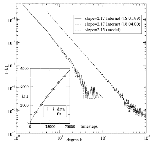
FIG. 1.: The degree distribution in the model with $r=0.29$ and $d=0.41$ and in the real Internet data collected on different days. In the inset there is the temporal behavior of the degree of a provider.

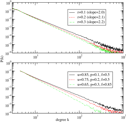
FIG. 2.: (above) Degree distribution for different values of the providers birth rate $r$ allowing users to have more than one provider. (below) Degree distribution with different user birth rates $u=1-r$ and probability of merging $f$.

REFERENCES

- [1] D.J. Watts, Small Worlds, Princeton University Press,
- [2] I. Rodriguez-Iturbe and A. Rinaldo, Fractal River Basins, Chance and Self-Organization, Cambridge University Press, Cambridge (1997).
- [3] J.R. Banavar, A. Maritan, A.Rinaldo Nature, 399 130 (1999).
- [4] M. Faloutsos, P. Faloutsos, C. Faloutsos ACM SIGCOMM ’99 Comput. Commun Rev., 29 251 (1999).
- [5] G. Caldarelli, R. Marchetti, L. Pietronero, Europhys. Lett., 52 386 (2000)
- [6] L. N. A. Amaral, A. Scala, M. Barthelemy, H. E. Stanley Proc. Nat. Acad. Sci. U.S.A. 97, 11149 (2000).
- [7] A description of the project, together with maps done by B. Cheswick and H. Burch are available at http://www.cs.bell-labs.com/who/ches/map/index.html
- [8] Simon, H.A., Biometrika 42, 425-440 (1955)
- [9] R. Albert, H. Jeong H. and A.-L. Barabási, Nature, 401 (1999) 130.
- [10] S. Bornholdt and H. Ebel, cond-mat/0008465.
- [11] S.N. Dorogotsev, J.F.F. Mendes, and A.N. Samukhin, cond-mat/0009090
- [12] M.E.J. Newman cond-mat/0011144.
- [13] B.A. Huberman and L.A. Adamic, Nature, 401 (1999) 131
- [14] A.-L. Barabási and R. Albert, Science 286, 509-512 (1999).
- [15] A.-L. Barabási and R. Albert, Phys. Rev. Lett. 85, 5234 (2000).
- [16] D.J. Watts and S.H. Strogatz, Nature, 393 (1998) 440.
- [17] A. Maritan, A. Rinaldo, R. Rigon, A. Giacometti, I. Rodriguez-Iturbe, Phys. Rev. E, 53 1510 (1996).
- [18] P. Erdös, R. Renyi Publ. Math. Inst. Hung. Acad. Sci., 5 (1960).
- [19] Data are available at the following URL http://moat.nlanr.net/Routing/rawdat
- [20] S.N.Dorogotsev and J.F.F. Mendes, Phys. Rev. E 62, 1842 (2000), cond-mat/0001419
- [21] P.L. Krapivsky, S.Redner, and F. Leyraz, cond-mat/0005139