Transmission Probability for Interacting Electrons
Connected to Reservoirs

1 Introduction

Effects of electron correlation on transport through small interacting systems have been a subject of current interest. For instance, the Kondo effect${}^{\hbox{\immediate{\bf{?}})}}$ in quantum dots has been studied intensively, and recent experiments${}^{\hbox{\immediate{\bf{?}},\penalty 1000\hskip 0.91003pt plus 0.70004pt minus 0.70004pt{\bf{?}},\penalty 1000\hskip 0.91003pt plus 0.70004pt minus 0.70004pt{\bf{?}})}}$ have demonstrated a qualitative agreement with theoretical predictions.${}^{\hbox{\immediate{\bf{?}},\penalty 1000\hskip 0.91003pt plus 0.70004pt minus 0.70004pt{\bf{?}},\penalty 1000\hskip 0.91003pt plus 0.70004pt minus 0.70004pt{\bf{?}})}}$

To investigate transport properties of small systems, it is essential to use theoretical approaches which are able to treat correctly both the interaction and quantum interference effects. The Keldysh formalism${}^{\hbox{\immediate{\bf{?}})}}$ has been applied to nonequilibrium systems.${}^{\hbox{\immediate{\bf{?}},\penalty 1000\hskip 0.91003pt plus 0.70004pt minus 0.70004pt{\bf{?}})}}$ Caroli et al have shown for noninteracting electrons that the current is determined by single-particle excitations between the two chemical potentials of the left and right leads.${}^{\hbox{\immediate{?})}}$ However, to our knowledge, the same feature has been shown to hold for interacting electrons only in a special case where the hopping matrix elements, which connects an interacting region at the center and the two leads, satisfy a certain condition.${}^{\hbox{\immediate{?})}}$ Although this condition for the connectivity is not so important for a single Anderson impurity, it restricts the application of the formulation to interacting systems consisting of a number of quantum levels. Our motivation of a series of works is based on a conjecture: as far as the linear response is concerned, the current through small interacting systems may be determined by low-lying states near the Fermi energy. It has been clarified without the assumption of the connectivity that the conductance is written in terms of the Green’s function at the Fermi energy $\epsilon=0$, at zero temperature $T=0$.${}^{\hbox{\immediate{\bf{?}},\penalty 1000\hskip 0.91003pt plus 0.70004pt minus 0.70004pt{\bf{?}})}}$ This is caused by a ground-state property of Fermi systems, i.e., the imaginary part of the self-energy vanishes at $\epsilon=0$, $T=0$.${}^{\hbox{\immediate{\bf{?}})}}$ Consequently, the contribution of the vertex corrections vanishes. The proof was provided based on the Kubo formalism making use of the diagrammatic analysis,${}^{\hbox{\immediate{\bf{?}},\penalty 1000\hskip 0.91003pt plus 0.70004pt minus 0.70004pt{\bf{?}})}}$ and it justifies an interpretation of the conductance in terms of the free quasi-particles.${}^{\hbox{\immediate{\bf{?}},\penalty 1000\hskip 0.91003pt plus 0.70004pt minus 0.70004pt{\bf{?}})}}$

The purpose of this paper is to generalize the formulation to finite temperatures. To this end, we have carried out the analytic continuation of the vertex part making use of a Éliashberg theory of the analytic properties, which was originally proposed to the translational invariant Fermi systems${}^{\hbox{\immediate{\bf{?}})}}$ and extended to lattice systems.${}^{\hbox{\immediate{\bf{?}})}}$ Compared to these examples, the situation we are considering is different in the following points: systems have no translational symmetry, and noninteracting leads connected to the interacting region keep the initial and final scattering states unrenormalized. One of the main results is that the conductance can be expressed as eq. (2.37) using the transmission probability ${\cal T}(\epsilon)$ which is defined in terms of a current vertex eq. (2.38) or a three-point correlation function eq. (3.6). It can be also written in the Lehmann representation as eq. (6.6).

We apply the formulation to a series of Anderson impurities of size $N$ (=1,2,3,4). For $N\geq 2$, the off-diagonal (non-local) elements of the self-energy and current vertex play important roles on the transport properties.${}^{\hbox{\immediate{?})}}$ Therefore, it is essential to perform calculations with a current-conserving approach. We calculate ${\cal T}(\epsilon)$ in an electron-hole symmetric case using the order $U^{2}$ self-energy and current vertex which satisfy a generalized Ward identity. At low temperatures, the value of the conductance is determined by the low energy part of ${\cal T}(\epsilon)$ because of the Fermi factor $-\partial f/\partial\epsilon$ in eq. (2.37). Nevertheless, the high energy part of ${\cal T}(\epsilon)$ also has much information about the excitation spectrum of interacting electrons: ${\cal T}(\epsilon)$ has two broad peaks of the upper and lower Hubbard bands in addition to $N$ resonant peaks which have direct correspondence with the noninteracting spectrum. At low temperatures, the peak structures near the Fermi energy depend on whether $N$ is even or odd: the Kondo peak is situated at $\epsilon=0$ for odd $N$ while it is a valley for even $N$. The even-odd oscillation becomes small with increasing $T$ and disappears at high temperatures $T\mathrel{\mathchoice{\lower 3.0pt\vbox{\halign{$\m@th\displaystyle\hfill#\hfil$\cr>\crcr\sim\crcr}}}{\lower 3.0pt\vbox{\halign{$\m@th\textstyle\hfill#\hfil$\cr>\crcr\sim\crcr}}}{\lower 3.0pt\vbox{\halign{$\m@th\scriptstyle\hfill#\hfil$\cr>\crcr\sim\crcr}}}{\lower 3.0pt\vbox{\halign{$\m@th\scriptscriptstyle\hfill#\hfil$\cr>\crcr\sim\crcr}}}}T_{K}$, where $T_{K}$ is the Kondo temperature.

In §2, we describe the formulation, and introduce the transmission probability ${\cal T}(\epsilon)$ carrying out the analytic continuation of the vertex part. In §3, the alternative expression of ${\cal T}(\epsilon)$ is given in terms of a three-point correlation function, and the current conservation is discussed in terms of a generalized Ward identity. In §4, we apply the formulation to a linear chain of the Anderson impurities. Summary is given in §5. The Lehmann representation of ${\cal T}(\epsilon)$ is given in Appendix.

2 Conductance and Transmission Probability

In this section we describe a finite temperature formulation for the current through small interacting systems connected to reservoirs based on the linear response theory. We perform the analytic continuation of the vertex part following Éliashberg,${}^{\hbox{\immediate{?})}}$ and introduce the transmission probability for interacting electrons, ${\cal T}(\epsilon)$, by which the conductance can be expressed in a Landauer type form.${}^{\hbox{\immediate{\bf{?}},\penalty 1000\hskip 0.91003pt plus 0.70004pt minus 0.70004pt{\bf{?}},\penalty 1000\hskip 0.91003pt plus 0.70004pt minus 0.70004pt{\bf{?}})}}$

2.1 Model

We start with a system which consists of three regions; a finite central region ($C$) and two reservoirs on the left ($L$) and the right ($R$). The central region consists of $N$ resonant levels, and the interaction $U_{j_{4}j_{3};j_{2}j_{1}}$ is switched on only for the electrons in this region. We assume that each of the reservoirs is infinitely large and has a continuous energy spectrum. The central region and the reservoirs are connected with the mixing matrix elements $v_{L}^{\phantom{\dagger}}$ and $v_{R}^{\phantom{\dagger}}$, as illustrated in Fig. 1. The Hamiltonian is given by

$${\cal H}\ = \ {\cal H}_{L}+{\cal H}_{R}+{\cal H}_{C}^{0}+{\cal H}_{C}^{int}+{\cal H}_{mix}\;,$$ (2.1)

$${\cal H}_{L} = \sum_{ij\in L}\sum_{\sigma}\left(\,-t_{ij}^{L}-\mu\,\delta_{ij}\,\right)c^{\dagger}_{i\sigma}c^{\phantom{\dagger}}_{j\sigma}\;,$$ (2.2)

$${\cal H}_{R} = \sum_{ij\in R}\sum_{\sigma}\left(\,-t_{ij}^{R}-\mu\,\delta_{ij}\,\right)c^{\dagger}_{i\sigma}c^{\phantom{\dagger}}_{j\sigma}\;,$$ (2.3)

$${\cal H}_{C}^{0} = \sum_{ij\in C}\sum_{\sigma}\left(\,-t_{ij}^{C}-\mu\,\delta_{ij}\,\right)c^{\dagger}_{i\sigma}c^{\phantom{\dagger}}_{j\sigma}\;,$$ (2.4)

$${\cal H}_{C}^{int} = {1\over 2}\sum_{\{j\}\in C}\sum_{\sigma\sigma^{\prime}}U_{j_{4}j_{3};j_{2}j_{1}}\,c^{\dagger}_{j_{4}\sigma}c^{\dagger}_{j_{3}\sigma^{\prime}}c^{\phantom{\dagger}}_{j_{2}\sigma^{\prime}}c^{\phantom{\dagger}}_{j_{1}\sigma}\;,$$ (2.5)

$${\cal H}_{mix} = -\sum_{\sigma}v_{L}^{\phantom{\dagger}}\left(\,c^{\dagger}_{1\sigma}c^{\phantom{\dagger}}_{0\sigma}+c^{\dagger}_{0\sigma}c^{\phantom{\dagger}}_{1\sigma}\,\right)-\sum_{\sigma}v_{R}^{\phantom{\dagger}}\left(\,c^{\dagger}_{N+1\sigma}c^{\phantom{\dagger}}_{N\sigma}+c^{\dagger}_{N\sigma}c^{\phantom{\dagger}}_{N+1\sigma}\,\right).$$ (2.6)

Here $c^{\dagger}_{j\sigma}$ ($c^{\phantom{\dagger}}_{j\sigma}$) creates (destroys) an electron with spin $\sigma$ at site $j$, and $\mu$ is the chemical potential. $t_{ij}^{L}$, $t_{ij}^{R}$, and $t_{ij}^{C}$ are the intra-region hopping matrix elements in each regions $L$, $R$, and $C$, respectively. The labels $1$, $2$, $\ldots$, $N$ are assigned to the sites in the central region. Specifically, the label $1$ ($N$) is assigned to the site at the interface on the left (right), and the label $0$ ($N+1$) is assigned to the site at the reservoir-side of the left (right) interface. We assume that the hopping matrix elements are real, and the interaction has the time-reversal symmetry: $U_{43;21}$ is real and $U_{43;21}=U_{34;12}=U_{12;34}=U_{42;31}=U_{13;24}$. We will be using units $\hbar=1$ unless otherwise noted.

The single-particle Green’s function is defined by

$$G_{jj^{\prime}}({\rm i}\varepsilon_{m})=-\int_{0}^{\beta}\!{\rm d}\tau\left\langle T_{\tau}\,c^{\phantom{\dagger}}_{j\sigma}(\tau)\,c^{\dagger}_{j^{\prime}\sigma}(0)\right\rangle\,{\rm e}^{{\rm i}\,\varepsilon_{m}\tau}.$$ (2.7)

Here $\beta=1/T$, $\varepsilon_{m}=(2m+1)\pi/\beta$, $c_{j\sigma}(\tau)={\rm e}^{\tau{\cal H}}c_{j\sigma}{\rm e}^{-\tau{\cal H}}$, and $\langle\cdots\rangle$ denotes the thermal average $\mbox{Tr}\left[\,{\rm e}^{-\beta{\cal H}}\,{\cdots}\,\right]/\mbox{Tr}\,{\rm e}^{-\beta{\cal H}}$. The spin index has been omitted from the left-hand side of eq. (2.7) assuming the expectation value to be independent of whether spin is up or down. Since the interaction is switched on only for the electrons in the central region, the Dyson equation can be written as

$$G_{ij}(z)=G^{0}_{ij}(z)+\sum_{i^{\prime}j^{\prime}\in C}\,G^{0}_{ii^{\prime}}(z)\,\Sigma_{i^{\prime}j^{\prime}}(z)\,G_{j^{\prime}j}(z)\;.$$ (2.8)

Here $G^{0}_{ij}(z)$ is the unperturbed Green’s function corresponding to the noninteracting Hamiltonian ${\cal H}^{0}\equiv{\cal H}_{L}+{\cal H}_{R}+{\cal H}_{C}^{0}+{\cal H}_{mix}$. The summations with respect to $i^{\prime}$ and $j^{\prime}$ run over the sites in the central region, and $\Sigma_{i^{\prime}j^{\prime}}(z)$ is the self-energy due to the interaction ${\cal H}_{C}^{int}$. Owing to the time-reversal symmetry of ${\cal H}$, these functions are symmetric against the interchange of the site indices: $G_{ij}(z)=G_{ji}(z)$ and $\Sigma_{ij}(z)=\Sigma_{ji}(z)$. Note that at $T=0$ the single-particle excitation at the Fermi energy $z={\rm i}0^{+}$ does not decay, i.e., $\mbox{Im}\,\Sigma_{ij}^{+}(0)=0$.${}^{\hbox{\immediate{?})}}$ We will treat $z$ as a complex variable, and use the symbol $+$ ($-$) in the superscript as a label for the retarded (advanced) function: $\Sigma_{ij}^{\pm}(\epsilon)\equiv\Sigma_{ij}(\epsilon\pm{\rm i}0^{+})$.

2.2 Analytic continuation of the vertex part

We next consider the conductance based on the Kubo formalism. The conductance $g$ is given by the $\omega$-linear imaginary part of a current-current correlation function:

$$g\ = \ e^{2}\,\lim_{\omega\to 0}{K_{\alpha\alpha^{\prime}}(\omega+{\rm i}0^{+})-K_{\alpha\alpha^{\prime}}({\rm i}0^{+})\over{\rm i}\,\omega}\;,$$ (2.9)

$$K_{\alpha\alpha^{\prime}}({\rm i}\nu_{l}) = \int_{0}^{\beta}\!{\rm d}\tau\left\langle T_{\tau}\,J_{\alpha}(\tau)J_{\alpha^{\prime}}(0)\right\rangle\,{\rm e}^{{\rm i}\,\nu_{l}\tau}.$$ (2.10)

Here $\nu_{l}=2\pi l/\beta$ is the Matsubara frequency, and the retarded function can be obtained through the analytic continuation $K_{\alpha\alpha^{\prime}}(\omega+{\rm i}0^{+})\equiv\left.K_{\alpha\alpha^{\prime}}({\rm i}\nu_{l})\right|_{{\rm i}\nu_{l}\to\omega+{\rm i}0^{+}}$. The current operator $J_{\alpha}$, for $\alpha=L$ or $R$, is defined by

$$J_{L} = {\rm i}\,\sum_{\sigma}v_{L}^{\phantom{\dagger}}\left(\,c^{\dagger}_{1\sigma}c^{\phantom{\dagger}}_{0\sigma}-c^{\dagger}_{0\sigma}c^{\phantom{\dagger}}_{1\sigma}\,\right),$$ (2.11)

$$J_{R} = {\rm i}\,\sum_{\sigma}v_{R}^{\phantom{\dagger}}\left(\,c^{\dagger}_{N+1\sigma}c^{\phantom{\dagger}}_{N\sigma}-c^{\dagger}_{N\sigma}c^{\phantom{\dagger}}_{N+1\sigma}\,\right).$$ (2.12)

Here $J_{L}$ is the current flowing into the sample from the left lead, and $J_{R}$ is the current flowing out to the right lead from the sample. These currents and total charge in the sample, $\rho_{C}^{\phantom{0}}=\sum_{j\in C,\sigma}c^{\dagger}_{j\sigma}c^{\phantom{\dagger}}_{j\sigma}$, satisfy the equation of continuity ${\partial\rho_{C}^{\phantom{0}}/\partial t}+J_{R}-J_{L}=0$. Due to this property, the value of $g$ given by eq. (2.9) is independent of $\alpha$ and $\alpha^{\prime}$.${}^{\hbox{\immediate{?})}}$ Note that $K_{\alpha^{\prime}\alpha}(z)=K_{\alpha\alpha^{\prime}}(z)$ because of the time-reversal symmetry of ${\cal H}$.

We calculate the $\omega$-linear part of $K_{\alpha\alpha^{\prime}}(z)$ taking $\alpha$ and $\alpha^{\prime}$ to be $R$ and $L$. The function $K_{RL}({\rm i}\nu)$ can be separated into the two terms as shown in Fig. 2:

$$K_{RL}({\rm i}\nu) = \ K_{RL}^{(a)}({\rm i}\nu)\ +\ K_{RL}^{(b)}({\rm i}\nu)\;,$$ (2.13)

$$K_{RL}^{(a)}({\rm i}\nu) = -\,({\rm i}\,v_{L}^{\phantom{\dagger}})\,({\rm i}\,v_{R}^{\phantom{\dagger}})\ {1\over\beta}\sum_{{\rm i}\varepsilon}\sum_{\sigma}$$ (2.14)

$$\times\Bigl{[}\,G_{N,1}({\rm i}\varepsilon+{\rm i}\nu)\,G_{0,N+1}({\rm i}\varepsilon)+G_{N+1,0}({\rm i}\varepsilon+{\rm i}\nu)\,G_{1,N}({\rm i}\varepsilon)$$

$$\quad-G_{N+1,1}({\rm i}\varepsilon+{\rm i}\nu)\,G_{0,N}({\rm i}\varepsilon)-G_{N,0}({\rm i}\varepsilon+{\rm i}\nu)\,G_{1,N+1}({\rm i}\varepsilon)\,\Bigr{]}\;,$$

$$K_{RL}^{(b)}({\rm i}\nu) = -\,({\rm i}\,v_{L}^{\phantom{\dagger}})\,({\rm i}\,v_{R}^{\phantom{\dagger}})\ {1\over\beta^{2}}\sum_{{\rm i}\varepsilon,{\rm i}\varepsilon^{\prime}}\sum_{\sigma\sigma^{\prime}}\sum_{\{j\}\in C}$$ (2.15)

$$\times\Bigl{[}\,G_{j_{1},1}({\rm i}\varepsilon+{\rm i}\nu)\,G_{0,j_{4}}({\rm i}\varepsilon)-G_{j_{1},0}({\rm i}\varepsilon+{\rm i}\nu)\,G_{1,j_{4}}({\rm i}\varepsilon)\,\Bigr{]}$$

$$\times\,\Gamma^{\sigma\sigma^{\prime}}_{j_{1}j_{2};\,j_{3}j_{4}}({\rm i}\varepsilon,{\rm i}\varepsilon^{\prime};{\rm i}\nu)$$

$$\times\Bigl{[}\,G_{N,j_{2}}({\rm i}\varepsilon^{\prime}+{\rm i}\nu)\,G_{j_{3},N+1}({\rm i}\varepsilon^{\prime})-G_{N+1,j_{2}}({\rm i}\varepsilon^{\prime}+{\rm i}\nu)\,G_{j_{3},N}({\rm i}\varepsilon^{\prime})\,\Bigr{]}\;.$$

Here $\Gamma^{\sigma\sigma^{\prime}}_{j_{1}j_{2};\,j_{3}j_{4}}({\rm i}\varepsilon,{\rm i}\varepsilon^{\prime};{\rm i}\nu)$ is the total vertex part due to ${\cal H}_{C}^{int}$, and the summation with respect to $\{j\}$ runs over the sites in the central region $j_{1},\ldots,j_{4}\in C$. Since the leads are assumed to be noninteracting, the Green’s function satisfies the following relations at the two interfaces:

$$\left\{\begin{array}[]{ll}G_{0,j}(z)\phantom{{}_{+1}}=-\mbox{\sl g}_{L}(z)\,v_{L}^{\phantom{\dagger}}G_{1,j}(z)&\quad\mbox{for}\quad 1\leq j\leq N+1\\ G_{j,N+1}(z)=-G_{j,N}(z)\,v_{R}^{\phantom{\dagger}}\,\mbox{\sl g}_{R}(z)&\quad\mbox{for}\quad 0\leq j\leq N\\ \end{array}\right.\;\;.$$ (2.18)

Here $\mbox{\sl g}_{L}(z)$ and $\mbox{\sl g}_{R}(z)$ are the local Green’s functions at the interfaces of the isolated leads, $0$ and $N+1$, respectively. Using these relations, $K_{RL}({\rm i}\nu)$ can be rewritten in terms of the Green’s functions in the central region as

$$K_{RL}({\rm i}\nu) = \ {1\over\beta}\sum_{{\rm i}\varepsilon}\sum_{\sigma}\sum_{j_{1}j_{4}\in C}\lambda_{L}({\rm i}\varepsilon,{\rm i}\varepsilon+{\rm i}\nu)\,G_{1j_{4}}({\rm i}\varepsilon)\,\Lambda_{R;j_{4}j_{1}}({\rm i}\varepsilon,{\rm i}\varepsilon+{\rm i}\nu)\,G_{j_{1}1}({\rm i}\varepsilon+{\rm i}\nu)\;.$$ (2.19)

Here the bare and full current vertices are defined by

$$\lambda_{L}({\rm i}\varepsilon,{\rm i}\varepsilon+{\rm i}\nu) = -{\rm i}\,v_{L}^{2}\left[\,\mbox{\sl g}_{L}({\rm i}\varepsilon+{\rm i}\nu)-\mbox{\sl g}_{L}({\rm i}\varepsilon)\,\right]\;,$$ (2.20)

$$\lambda_{R}({\rm i}\varepsilon,{\rm i}\varepsilon+{\rm i}\nu) = \ {\rm i}\,v_{R}^{2}\left[\,\mbox{\sl g}_{R}({\rm i}\varepsilon+{\rm i}\nu)-\mbox{\sl g}_{R}({\rm i}\varepsilon)\,\right]\;,$$ (2.21)

$$\Lambda_{R;j_{4}j_{1}}({\rm i}\varepsilon,{\rm i}\varepsilon+{\rm i}\nu) = \,\lambda_{R}({\rm i}\varepsilon,{\rm i}\varepsilon+{\rm i}\nu)\,\delta_{Nj_{4}}\delta_{Nj_{1}}\,+\,P_{j_{4}j_{1}}({\rm i}\varepsilon,{\rm i}\varepsilon+{\rm i}\nu)\;,$$ (2.22)

$$P_{j_{4}j_{1}}({\rm i}\varepsilon,{\rm i}\varepsilon+{\rm i}\nu) = \,{1\over\beta}\sum_{{\rm i}\varepsilon^{\prime}}\sum_{\sigma^{\prime}}\sum_{j_{2}j_{3}\in C}\,\Gamma^{\sigma\sigma^{\prime}}_{j_{1}j_{2};\,j_{3}j_{4}}({\rm i}\varepsilon,{\rm i}\varepsilon^{\prime};{\rm i}\nu)$$ (2.23)

$$\times\,G_{j_{3}N}({\rm i}\varepsilon^{\prime})\,\lambda_{R}({\rm i}\varepsilon^{\prime},{\rm i}\varepsilon^{\prime}+{\rm i}\nu)\,G_{Nj_{2}}({\rm i}\varepsilon^{\prime}+{\rm i}\nu)\;.$$

The spin index has been omitted from the left-hand side of eq. (2.23) since it is independent of $\sigma$ due to the rotational symmetry of the spin space. The $\omega$-linear part of the retarded function $K_{RL}(\omega+i0^{+})$ can be obtained from eq. (2.19) by carrying out the analytic continuation:

$$K_{RL}(\omega+i0^{+}) = \sum_{\sigma}\sum_{j_{1}j_{4}\in C}\biggl{\{}$$ (2.24)

$$-\int_{-\infty}^{\infty}{{\rm d}\epsilon\over 2\pi{\rm i}}\ f(\epsilon)\ \lambda_{L}^{[1]}(\epsilon,\epsilon+\omega)\,G_{1j_{4}}^{+}(\epsilon)\,\Lambda_{R;j_{4}j_{1}}^{[1]}(\epsilon,\epsilon+\omega)\,G_{j_{1}1}^{+}(\epsilon+\omega)$$

$$-\int_{-\infty}^{\infty}{{\rm d}\epsilon\over 2\pi{\rm i}}\,\Bigl{[}\,f(\epsilon+\omega)-f(\epsilon)\,\Bigr{]}\ \lambda_{L}^{[2]}(\epsilon,\epsilon+\omega)\,G_{1j_{4}}^{-}(\epsilon)\,\Lambda_{R;j_{4}j_{1}}^{[2]}(\epsilon,\epsilon+\omega)\,G_{j_{1}1}^{+}(\epsilon+\omega)$$

$$+\int_{-\infty}^{\infty}{{\rm d}\epsilon\over 2\pi{\rm i}}\ f(\epsilon+\omega)\ \lambda_{L}^{[3]}(\epsilon,\epsilon+\omega)\,G_{1j_{4}}^{-}(\epsilon)\,\Lambda_{R;j_{4}j_{1}}^{[3]}(\epsilon,\epsilon+\omega)\,G_{j_{1}1}^{-}(\epsilon+\omega)\,\biggr{\}}.$$

Here $f(\epsilon)=[{\rm e}^{\beta\epsilon}+1]^{-1}$. The superscript [k] for $k=1,2,3$ is introduced for the current vertices in order to specify the three analytic regions of $\Lambda_{R;j_{4}j_{1}}(z,z+w)$ in the complex $z$-plane, which are separated by the two lines, $\mbox{Im}\,(z)=0$ and $\mbox{Im}\,(z+w)=0$, as shown in Fig 3. The explicit form of the bare current vertex is given by

$$\lambda_{\alpha}^{[k]}(\epsilon,\epsilon+\omega)\propto\left\{\begin{array}[]{ll}\,\mbox{\sl g}_{\alpha}^{+}(\epsilon+\omega)-\mbox{\sl g}_{\alpha}^{+}(\epsilon)&\quad\mbox{for}\quad k=1\\ \,\mbox{\sl g}_{\alpha}^{+}(\epsilon+\omega)-\mbox{\sl g}_{\alpha}^{-}(\epsilon)&\quad\mbox{for}\quad k=2\\ \,\mbox{\sl g}_{\alpha}^{-}(\epsilon+\omega)-\mbox{\sl g}_{\alpha}^{-}(\epsilon)&\quad\mbox{for}\quad k=3\end{array}\right.\;,$$ (2.25)

for $\alpha=L,R$. Thus, in the limit of $\omega\to 0$, $\lambda_{\alpha}^{[1]}(\epsilon,\epsilon)=0$ and $\lambda_{\alpha}^{[3]}(\epsilon,\epsilon)=0$. Furthermore, $\lambda_{R}^{[2]}(\epsilon,\epsilon)=2\,\Gamma_{R}(\epsilon)$ and $\lambda_{L}^{[2]}(\epsilon,\epsilon)=-2\,\Gamma_{L}(\epsilon)$ with $\Gamma_{\alpha}(\epsilon)=-\,\mbox{Im}\left[v_{\alpha}^{2}\,\mbox{\sl g}_{\alpha}^{+}(\epsilon)\right]$. In order to calculate the $\omega$-linear part of eq. (2.24), we next consider the behavior of $P_{j_{4}j_{1}}^{[k]}(\epsilon,\epsilon+\omega)$ for small $\omega$ carrying out the analytic continuation of $P_{j_{4}j_{1}}({\rm i}\varepsilon,{\rm i}\varepsilon+{\rm i}\nu)$ using eq. (2.23). It can be done following the Éliashberg theory of the analytic properties of the vertex part.${}^{\hbox{\immediate{?})}}$ As a function of the complex variables, $\Gamma^{\sigma\sigma^{\prime}}_{j_{1}j_{2};\,j_{3}j_{4}}(z,z^{\prime};w)$ has singularities along the lines shown in Fig. 4: the vertical lines $\mbox{Im}\,(z)=0$ and $\mbox{Im}\,(z+w)=0$, the horizontal lines $\mbox{Im}\,(z^{\prime})=0$ and $\mbox{Im}\,(z^{\prime}+w)=0$, and the diagonal lines $\mbox{Im}\,(z-z^{\prime})=0$ and $\mbox{Im}\,(z+z^{\prime}+w)=0$. These lines divide the plane into 16 regions, each of which corresponds to a function of $\Gamma^{\sigma\sigma^{\prime}}_{j_{1}j_{2};\,j_{3}j_{4}}(z,z^{\prime};w)$ which is analytic in that region in any of its arguments. The rectangular regions in Fig. 4 are numbered by indices $[k,k^{\prime}]$ for $k,k^{\prime}=1,2,3$. Some of these regions are divided into parts by the diagonal lines, and these parts are denoted by Roman numbers. We will use this notation also for the vertex part in eqs. (2.27)–(2.35). Rewriting the summation over the Matsubara frequency ${\rm i}\varepsilon^{\prime}$ in eq.(2.23) in terms of a contour integral along these lines and then performing the analytic continuation, $P_{j_{4}j_{1}}^{[k]}(\epsilon,\epsilon+\omega)$ is obtained as

$$P_{j_{4}j_{1}}^{[k]}(\epsilon,\epsilon+\omega) = \sum_{\sigma^{\prime}}\sum_{j_{2}j_{3}\in C}\biggl{\{}\,$$ (2.26)

$$\phantom{+}\int_{-\infty}^{\infty}{{\rm d}\epsilon^{\prime}\over 2\pi{\rm i}}\ {\cal L}^{\sigma\sigma^{\prime}\,[k,1]}_{j_{1}j_{2};\,j_{3}j_{4}}(\epsilon,\epsilon^{\prime};\omega)\ G_{j_{3}N}^{+}(\epsilon^{\prime})\,\lambda_{R}^{[1]}(\epsilon^{\prime},\epsilon^{\prime}+\omega)\,G_{Nj_{2}}^{+}(\epsilon^{\prime}+\omega)$$

$$+\int_{-\infty}^{\infty}{{\rm d}\epsilon^{\prime}\over 2\pi{\rm i}}\ {\cal L}^{\sigma\sigma^{\prime}\,[k,2]}_{j_{1}j_{2};\,j_{3}j_{4}}(\epsilon,\epsilon^{\prime};\omega)\ G_{j_{3}N}^{-}(\epsilon^{\prime})\,\lambda_{R}^{[2]}(\epsilon^{\prime},\epsilon^{\prime}+\omega)\,G_{Nj_{2}}^{+}(\epsilon^{\prime}+\omega)$$

$$+\int_{-\infty}^{\infty}{{\rm d}\epsilon^{\prime}\over 2\pi{\rm i}}\ {\cal L}^{\sigma\sigma^{\prime}\,[k,3]}_{j_{1}j_{2};\,j_{3}j_{4}}(\epsilon,\epsilon^{\prime};\omega)\ G_{j_{3}N}^{-}(\epsilon^{\prime})\,\lambda_{R}^{[3]}(\epsilon^{\prime},\epsilon^{\prime}+\omega)\,G_{Nj_{2}}^{-}(\epsilon^{\prime}+\omega)\,\biggr{\}}\;.$$

Here ${\cal L}^{\sigma\sigma^{\prime}\,[k,k^{\prime}]}_{j_{1}j_{2};\,j_{3}j_{4}}(\epsilon,\epsilon^{\prime};\omega)$ is defined by

$${\cal L}^{\sigma\sigma^{\prime}\,[11]}_{j_{1}j_{2};\,j_{3}j_{4}}(\epsilon,\epsilon^{\prime};\omega) = {\cal P}b(\epsilon^{\prime}-\epsilon)\left[\,\Gamma^{\sigma\sigma^{\prime}[11;\,\mbox{II}]}_{j_{1}j_{2};\,j_{3}j_{4}}(\epsilon,\epsilon^{\prime};\omega)-\Gamma^{\sigma\sigma^{\prime}[11;\,\mbox{I}]}_{j_{1}j_{2};\,j_{3}j_{4}}(\epsilon,\epsilon^{\prime};\omega)\,\right]$$ (2.27)

$$-f(\epsilon^{\prime})\,\Gamma^{\sigma\sigma^{\prime}[11;\,\mbox{I}]}_{j_{1}j_{2};\,j_{3}j_{4}}(\epsilon,\epsilon^{\prime};\omega)\;,$$

$${\cal L}^{\sigma\sigma^{\prime}\,[12]}_{j_{1}j_{2};\,j_{3}j_{4}}(\epsilon,\epsilon^{\prime};\omega) = -\left[\,f(\epsilon^{\prime}+\omega)-f(\epsilon^{\prime})\,\right]\,\Gamma^{\sigma\sigma^{\prime}[12]}_{j_{1}j_{2};\,j_{3}j_{4}}(\epsilon,\epsilon^{\prime};\omega)\;,$$ (2.28)

$${\cal L}^{\sigma\sigma^{\prime}\,[13]}_{j_{1}j_{2};\,j_{3}j_{4}}(\epsilon,\epsilon^{\prime};\omega) = {\cal P}b(\epsilon^{\prime}+\epsilon+\omega)\left[\,\Gamma^{\sigma\sigma^{\prime}[13;\,\mbox{I}]}_{j_{1}j_{2};\,j_{3}j_{4}}(\epsilon,\epsilon^{\prime};\omega)-\Gamma^{\sigma\sigma^{\prime}[13;\,\mbox{II}]}_{j_{1}j_{2};\,j_{3}j_{4}}(\epsilon,\epsilon^{\prime};\omega)\,\right]$$ (2.29)

$$+f(\epsilon^{\prime}+\omega)\,\Gamma^{\sigma\sigma^{\prime}[13;\,\mbox{I}]}_{j_{1}j_{2};\,j_{3}j_{4}}(\epsilon,\epsilon^{\prime};\omega)\;,$$

$${\cal L}^{\sigma\sigma^{\prime}\,[21]}_{j_{1}j_{2};\,j_{3}j_{4}}(\epsilon,\epsilon^{\prime};\omega) = -f(\epsilon^{\prime})\,\Gamma^{\sigma\sigma^{\prime}[21]}_{j_{1}j_{2};\,j_{3}j_{4}}(\epsilon,\epsilon^{\prime};\omega)\;,$$ (2.30)

$${\cal L}^{\sigma\sigma^{\prime}\,[22]}_{j_{1}j_{2};\,j_{3}j_{4}}(\epsilon,\epsilon^{\prime};\omega) = f(\epsilon^{\prime})\,\Gamma^{\sigma\sigma^{\prime}[22;\,\mbox{II}]}_{j_{1}j_{2};\,j_{3}j_{4}}(\epsilon,\epsilon^{\prime};\omega)-f(\epsilon^{\prime}+\omega)\,\Gamma^{\sigma\sigma^{\prime}[22;\,\mbox{IV}]}_{j_{1}j_{2};\,j_{3}j_{4}}(\epsilon,\epsilon^{\prime};\omega)$$ (2.31)

$$+{\cal P}b(\epsilon^{\prime}-\epsilon)\,\left[\,\Gamma^{\sigma\sigma^{\prime}[22;\,\mbox{II}]}_{j_{1}j_{2};\,j_{3}j_{4}}(\epsilon,\epsilon^{\prime};\omega)-\Gamma^{\sigma\sigma^{\prime}[22;\,\mbox{III}]}_{j_{1}j_{2};\,j_{3}j_{4}}(\epsilon,\epsilon^{\prime};\omega)\,\right]$$

$$+{\cal P}b(\epsilon^{\prime}+\epsilon+\omega)\,\left[\,\Gamma^{\sigma\sigma^{\prime}[22;\,\mbox{III}]}_{j_{1}j_{2};\,j_{3}j_{4}}(\epsilon,\epsilon^{\prime};\omega)-\Gamma^{\sigma\sigma^{\prime}[22;\,\mbox{IV}]}_{j_{1}j_{2};\,j_{3}j_{4}}(\epsilon,\epsilon^{\prime};\omega)\,\right],$$

$${\cal L}^{\sigma\sigma^{\prime}\,[23]}_{j_{1}j_{2};\,j_{3}j_{4}}(\epsilon,\epsilon^{\prime};\omega) = f(\epsilon^{\prime}+\omega)\,\Gamma^{\sigma\sigma^{\prime}[23]}_{j_{1}j_{2};\,j_{3}j_{4}}(\epsilon,\epsilon^{\prime};\omega)\;,$$ (2.32)

$${\cal L}^{\sigma\sigma^{\prime}\,[31]}_{j_{1}j_{2};\,j_{3}j_{4}}(\epsilon,\epsilon^{\prime};\omega) = {\cal P}b(\epsilon^{\prime}+\epsilon+\omega)\left[\,\Gamma^{\sigma\sigma^{\prime}[31;\,\mbox{II}]}_{j_{1}j_{2};\,j_{3}j_{4}}(\epsilon,\epsilon^{\prime};\omega)-\Gamma^{\sigma\sigma^{\prime}[31;\,\mbox{I}]}_{j_{1}j_{2};\,j_{3}j_{4}}(\epsilon,\epsilon^{\prime};\omega)\,\right]$$ (2.33)

$$-f(\epsilon^{\prime})\,\Gamma^{\sigma\sigma^{\prime}[31;\,\mbox{I}]}_{j_{1}j_{2};\,j_{3}j_{4}}(\epsilon,\epsilon^{\prime};\omega)\;,$$

$${\cal L}^{\sigma\sigma^{\prime}\,[32]}_{j_{1}j_{2};\,j_{3}j_{4}}(\epsilon,\epsilon^{\prime};\omega) = -\left[\,f(\epsilon^{\prime}+\omega)-f(\epsilon^{\prime})\,\right]\,\Gamma^{\sigma\sigma^{\prime}[32]}_{j_{1}j_{2};\,j_{3}j_{4}}(\epsilon,\epsilon^{\prime};\omega)\;,$$ (2.34)

$${\cal L}^{\sigma\sigma^{\prime}\,[33]}_{j_{1}j_{2};\,j_{3}j_{4}}(\epsilon,\epsilon^{\prime};\omega) = {\cal P}b(\epsilon^{\prime}-\epsilon)\left[\,\Gamma^{\sigma\sigma^{\prime}[33;\,\mbox{I}]}_{j_{1}j_{2};\,j_{3}j_{4}}(\epsilon,\epsilon^{\prime};\omega)-\Gamma^{\sigma\sigma^{\prime}[33;\,\mbox{II}]}_{j_{1}j_{2};\,j_{3}j_{4}}(\epsilon,\epsilon^{\prime};\omega)\,\right]$$ (2.35)

$$+f(\epsilon^{\prime}+\omega)\,\Gamma^{\sigma\sigma^{\prime}[33;\,\mbox{I}]}_{j_{1}j_{2};\,j_{3}j_{4}}(\epsilon,\epsilon^{\prime};\omega)\;.$$

Here ${\cal P}$ denotes the Cauchy principal value, and $b(\epsilon)=[{\rm e}^{\beta\epsilon}-1]^{-1}$. The Fermi and Bose distribution functions came through the summation over ${\rm i}\varepsilon^{\prime}$. We can now examine the behavior of $P_{j_{4}j_{1}}^{[k]}(\epsilon,\epsilon+\omega)$ for small $\omega$. The first and third terms of the right-hand side of eq. (2.26) vanish at $\omega=0$ because $\lambda_{R}^{[1]}(\epsilon,\epsilon)=0$ and $\lambda_{R}^{[3]}(\epsilon,\epsilon)=0$ as already mentioned. Furthermore, due to the factor $\left[\,f(\epsilon^{\prime}+\omega)-f(\epsilon^{\prime})\,\right]$ appearing in eqs. (2.28) and (2.34), ${\cal L}^{\sigma\sigma^{\prime}\,[12]}_{j_{1}j_{2};\,j_{3}j_{4}}(\epsilon,\epsilon^{\prime};0)=0$ and ${\cal L}^{\sigma\sigma^{\prime}\,[32]}_{j_{1}j_{2};\,j_{3}j_{4}}(\epsilon,\epsilon^{\prime};0)=0$. Therefore in the limit of $\omega\to 0$, $P_{j_{4}j_{1}}^{[1]}(\epsilon,\epsilon)=0$, $P_{j_{4}j_{1}}^{[3]}(\epsilon,\epsilon)=0$, and

$$P_{j_{4}j_{1}}^{[2]}(\epsilon,\epsilon)\,=\,2\sum_{\sigma^{\prime}}\sum_{j_{2}j_{3}\in C}\int_{-\infty}^{\infty}{{\rm d}\epsilon^{\prime}\over 2\pi{\rm i}}\ {\cal L}^{\sigma\sigma^{\prime}\,[22]}_{j_{1}j_{2};\,j_{3}j_{4}}(\epsilon,\epsilon^{\prime};0)\ G_{j_{3},N}^{-}(\epsilon^{\prime})\,\Gamma_{R}(\epsilon^{\prime})\,G_{N,j_{2}}^{+}(\epsilon^{\prime})\;.$$ (2.36)

Similarly, through eq. (2.22) we have, $\Lambda_{R;j_{4}j_{1}}^{[1]}(\epsilon,\epsilon)=0$, $\Lambda_{R;j_{4}j_{1}}^{[3]}(\epsilon,\epsilon)=0$, and $\Lambda_{R;j_{4}j_{1}}^{[2]}(\epsilon,\epsilon)=2\Gamma_{R}(\epsilon)\,\delta_{Nj_{4}}\delta_{Nj_{1}}+P_{j_{4}j_{1}}^{[2]}(\epsilon,\epsilon)$. Therefore, the $\omega$-linear part of $K_{RL}(\omega+i0^{+})$ comes only from the second term of the right-hand side of eq. (2.24), and thus the conductance can be expressed as

$$g\ = \ {2e^{2}\over h}\,\int_{-\infty}^{\infty}{\rm d}\epsilon\left(-\,{\partial f\over\partial\epsilon}\right){\cal T}(\epsilon)\;,$$ (2.37)

$${\cal T}(\epsilon) = \ \sum_{j_{1}j_{4}\in C}2\,\Gamma_{L}(\epsilon)\,G_{1j_{4}}^{-}(\epsilon)\,\Lambda_{R;j_{4}j_{1}}^{[2]}(\epsilon,\epsilon)\,G_{j_{1}1}^{+}(\epsilon)\;.$$ (2.38)

Among nine functions of ${\cal L}^{\sigma\sigma^{\prime}\,[kk^{\prime}]}_{j_{1}j_{2};\,j_{3}j_{4}}$ given by eqs. (2.27)–(2.35), only one function ${\cal L}^{\sigma\sigma^{\prime}\,[22]}_{j_{1}j_{2};\,j_{3}j_{4}}$ is relevant to the conductance through eq. (2.36). We note that $\Lambda_{R;jj^{\prime}}^{[2]}(\epsilon,\epsilon)=\left\{\Lambda_{R;j^{\prime}j}^{[2]}(\epsilon,\epsilon)\right\}^{*}$ due to the time-reversal symmetry (see also Appendix), and thus ${\cal T}(\epsilon)$ is real. The contributions of the bubble and vertex diagrams can be separated as ${\cal T}(\epsilon)={\cal T}^{(a)}(\epsilon)+{\cal T}^{(b)}(\epsilon)$,

$${\cal T}^{(a)}(\epsilon) = \ 4\,\Gamma_{L}(\epsilon)\,G_{1N}^{-}(\epsilon)\,\Gamma_{R}(\epsilon)\,G_{N1}^{+}(\epsilon)\;,$$ (2.39)

$${\cal T}^{(b)}(\epsilon) = \sum_{j_{1}j_{4}\in C}2\,\Gamma_{L}(\epsilon)\,G_{1j_{4}}^{-}(\epsilon)\,P_{j_{4}j_{1}}^{[2]}(\epsilon,\epsilon)\,G_{j_{1}1}^{+}(\epsilon)\;.$$ (2.40)

At low temperatures, the conductance is determined by the behavior of ${\cal T}(\epsilon)$ at small $\epsilon$ because of the Fermi factor $-\,\partial f/\partial\epsilon$ in eq. (2.37). Specifically, the vertex contribution vanishes at zero temperature.${}^{\hbox{\immediate{?})}}$ This can be reexamined as follows: at $\omega=0$, $\epsilon=0$ and $T=0$, the [2,2] vertex function vanishes, i.e., ${\cal L}^{\sigma\sigma^{\prime}\,[22]}_{j_{1}j_{2};\,j_{3}j_{4}}(0,\epsilon^{\prime};0)=0$, due to the restriction of the phase space by the distributions $f(\epsilon^{\prime})$ and $b(\epsilon^{\prime})$ in eq. (2.31). Thus from eqs. (2.36) and (2.40) we have, $P_{j_{4}j_{1}}^{[2]}(0,0)=0$ and ${\cal T}^{(b)}(0)=0$, at zero temperature.

In this section, we have assumed the time-reversal symmetry of $U_{j_{4}j_{3};j_{2}j_{1}}$, but not assumed the precise form of this interaction. Thus, the present formulation can be applicable to the interaction which vanishes smoothly at the interfaces. We have also assumed that the two leads are noninteracting. Due to this assumption, we have no wavefunction renormalization in eq. (2.38). If the interaction is switched on also in the leads, the wavefunction renormalization may be necessary to define the initial and final scattering states.${}^{\hbox{\immediate{?})}}$

3 Current Conservation and Ward Identity

In this section, we provide an alternative expression of the transmission probability ${\cal T}(\epsilon)$ in terms of a three-point correlation function, i.e., eq. (3.6). This expression may be suitable for nonperturbative calculations such as numerical renormalization group${}^{\hbox{\immediate{\bf{?}},\penalty 1000\hskip 0.91003pt plus 0.70004pt minus 0.70004pt{\bf{?}},\penalty 1000\hskip 0.91003pt plus 0.70004pt minus 0.70004pt{\bf{?}})}}$ and quantum Monte Carlo method.${}^{\hbox{\immediate{\bf{?}})}}$ The Lehmann representation of ${\cal T}(\epsilon)$ can be obtained using the correlation function, and it is given in Appendix. We also discuss the current conservation in terms of the generalized Ward identity eq. (3.7). This identity can be rewritten in the form of eq. (3.12), and it shows a relationship between the self-energy and current vertex.

The three-point correlation functions of the charge and currents are defined by

$$\Phi_{C;jj^{\prime}}(\tau;\tau_{1},\tau_{2}) = \left\langle T_{\tau}\,\delta\rho_{C}^{\phantom{0}}(\tau)\,c^{\phantom{\dagger}}_{j\sigma}(\tau_{1})\,c^{\dagger}_{j^{\prime}\sigma}(\tau_{2})\right\rangle,$$ (3.1)

$$\Phi_{L;jj^{\prime}}(\tau;\tau_{1},\tau_{2}) = \left\langle T_{\tau}\,J_{L}(\tau)\,c^{\phantom{\dagger}}_{j\sigma}(\tau_{1})\,c^{\dagger}_{j^{\prime}\sigma}(\tau_{2})\right\rangle,$$ (3.2)

$$\Phi_{R;jj^{\prime}}(\tau;\tau_{1},\tau_{2}) = \left\langle T_{\tau}\,J_{R}(\tau)\,c^{\phantom{\dagger}}_{j\sigma}(\tau_{1})\,c^{\dagger}_{j^{\prime}\sigma}(\tau_{2})\right\rangle,$$ (3.3)

where $\delta\rho_{C}^{\phantom{0}}\equiv\rho_{C}^{\phantom{0}}-\langle\rho_{C}^{\phantom{0}}\rangle$. The Fourier transform of these functions are given by

$$\Phi_{\gamma:jj^{\prime}}(\tau;\tau_{1},\tau_{2})={1\over\beta^{2}}\sum_{{\rm i}\varepsilon,{\rm i}\nu}\Phi_{\gamma:jj^{\prime}}({\rm i}\varepsilon,{\rm i}\varepsilon+{\rm i}\nu)\,{\rm e}^{-{\rm i}\,\varepsilon(\tau_{1}-\tau)}\,{\rm e}^{-{\rm i}\,(\varepsilon+\nu)(\tau-\tau_{2})}\;,$$ (3.4)

for $\gamma=C,L,R$. In what follows, we will discuss the correlation functions in the central region assuming $jj^{\prime}\in C$. The right-hand side of eqs. (3.2) and (3.3) contain the operators with respect to sites in the reservoirs, $0$ and $N+1$, through $J_{L}$ and $J_{R}$. The contributions of these two sites can be rewritten in terms of the Green’s functions with respect to the adjacent sites $1$ and $N$ using eq. (2.18) with the Feynman diagrams for $\Phi_{\gamma:jj^{\prime}}({\rm i}\varepsilon,{\rm i}\varepsilon+{\rm i}\nu)$. Therefore, these correlation functions can be expressed in terms of the current vertex introduced in §2 as

$$\Phi_{\gamma;jj^{\prime}}({\rm i}\varepsilon,{\rm i}\varepsilon+{\rm i}\nu)=\sum_{j_{4}j_{1}\in C}G_{jj_{4}}({\rm i}\varepsilon)\,\Lambda_{\gamma;j_{4}j_{1}}({\rm i}\varepsilon,{\rm i}\varepsilon+{\rm i}\nu)\,G_{j_{1}j^{\prime}}({\rm i}\varepsilon+{\rm i}\nu)\;.$$ (3.5)

Here $\Lambda_{R;j_{4}j_{1}}$ is the current vertex for $J_{R}$ given by eqs. (2.22) and (2.23). The functions $\Lambda_{L;j_{4}j_{1}}$ and $\Lambda_{C;j_{4}j_{1}}$ are defined by the similar expressions; the bare vertices are given by $\lambda_{L}({\rm i}\varepsilon,{\rm i}\varepsilon+{\rm i}\nu)\,\delta_{1j_{4}}\,\delta_{1j_{1}}$ and $\delta_{j_{4}j_{1}}$, respectively. Thus, the transmission probability, eq. (2.38), corresponds to the analytic continuation of eq. (3.5) in the region, ${\rm i}\varepsilon+{\rm i}\nu\to\epsilon+\omega+{\rm i}0^{+}$ and ${\rm i}\varepsilon\to\epsilon-i0^{+}$, as

$${\cal T}(\epsilon) = 2\,\Gamma_{L}(\epsilon)\,\Phi_{R;11}^{[2]}(\epsilon,\epsilon)\;.$$ (3.6)

The Lehmann representation of $\Phi_{R;11}^{[2]}(\epsilon,\epsilon)$ is presented in Appendix.

In the rest of this section, we discuss the current conservation in terms of these correlation functions. Using the equation of continuity in the Matsubara form $-\left({\partial/\partial\tau}\right)\delta\rho_{C}^{\phantom{0}}+{\rm i}\,J_{R}-{\rm i}\,J_{L}=0$, the generalized Ward identity is obtained as${}^{\hbox{\immediate{\bf{?}})}}$

$$-\,{\partial\over\partial\tau}\,\Phi_{C;jj^{\prime}}(\tau;\tau_{1},\tau_{2})\,+{\rm i}\,\Phi_{R;jj^{\prime}}(\tau;\tau_{1},\tau_{2})-{\rm i}\,\Phi_{L;jj^{\prime}}(\tau;\tau_{1},\tau_{2})$$ (3.7)

$$= \ \,\delta(\tau-\tau_{2})\,G_{jj^{\prime}}(\tau_{1},\tau)-\,\delta(\tau_{1}-\tau)\,G_{jj^{\prime}}(\tau,\tau_{2})\;.$$

The Fourier transform of this identity can be expressed, using $N\times N$ matrices, as

$${\rm i}\nu\,\mbox{\boldmath$\Phi$}_{C}({\rm i}\varepsilon,{\rm i}\varepsilon+{\rm i}\nu)+{\rm i}\,\mbox{\boldmath$\Phi$}_{R}({\rm i}\varepsilon,{\rm i}\varepsilon+{\rm i}\nu)-{\rm i}\,\mbox{\boldmath$\Phi$}_{L}({\rm i}\varepsilon,{\rm i}\varepsilon+{\rm i}\nu)\,=\,\mbox{\boldmath$G$}({\rm i}\varepsilon)-\mbox{\boldmath$G$}({\rm i}\varepsilon+{\rm i}\nu).$$ (3.8)

Here $\mbox{\boldmath$G$}(z)=\{G_{jj^{\prime}}(z)\}$, $\mbox{\boldmath$\Phi$}_{\gamma}(z,z+w)=\{\Phi_{\gamma;jj^{\prime}}(z,z+w)\}$, and $\mbox{\boldmath$\Lambda$}_{\gamma}(z,z+w)=\{\Lambda_{\gamma;jj^{\prime}}(z,z+w)\}$ for $jj^{\prime}\in C$. In this notation, eq. (3.5) is written as $\mbox{\boldmath$\Phi$}_{\gamma}(z,z+w)=\mbox{\boldmath$G$}(z)\,\mbox{\boldmath$\Lambda$}_{\gamma}(z,z+w)\,\mbox{\boldmath$G$}(z+w)$. Therefore eq. (3.8) can be rewritten as

$${\rm i}\nu\,\mbox{\boldmath$\Lambda$}_{C}({\rm i}\varepsilon,{\rm i}\varepsilon+{\rm i}\nu)+{\rm i}\,\mbox{\boldmath$\Lambda$}_{R}({\rm i}\varepsilon,{\rm i}\varepsilon+{\rm i}\nu)-{\rm i}\,\mbox{\boldmath$\Lambda$}_{L}({\rm i}\varepsilon,{\rm i}\varepsilon+{\rm i}\nu)=\left\{\mbox{\boldmath$G$}({\rm i}\varepsilon+{\rm i}\nu)\right\}^{-1}-\left\{\mbox{\boldmath$G$}({\rm i}\varepsilon)\right\}^{-1}.$$ (3.9)

Furthermore, the Dyson equation eq. (2.8) can be expressed as $\left\{\mbox{\boldmath$G$}(z)\right\}^{-1}=z\,\mbox{\boldmath$1$}-\mbox{\boldmath${\cal H}$}_{C}^{0}-\mbox{\boldmath${\cal V}$}_{mix}(z)-\mbox{\boldmath$\Sigma$}(z)$:

$$\mbox{\boldmath${\cal H}$}_{C}^{0}\ = \ \left[\,\matrix{-t_{11}^{C}-\mu&-t_{12}^{C}&\cdots&\cr-t_{21}^{C}&-t_{22}^{C}-\mu&&\cr\vdots&&\ddots&\cr&&&-t_{NN}^{C}-\mu\cr}\,\right]\;,$$ (3.10)

$$\mbox{\boldmath${\cal V}$}_{mix}(z)\ = \ \left[\,\matrix{v_{L}^{2}\,\mbox{\sl g}_{L}(z)&0&\cdots&0&0\cr 0&0&\cdots&0&0\cr\vdots&\vdots&\ddots&\vdots&\vdots\cr 0&0&\cdots&0&0\cr 0&0&\cdots&0&v_{R}^{2}\,\mbox{\sl g}_{R}(z)\cr}\,\right]\;,$$ (3.11)

and $\mbox{\boldmath$\Sigma$}(z)=\{\Sigma_{jj^{\prime}}(z)\}$. The mixing matrix $\mbox{\boldmath${\cal V}$}_{mix}$ has only two non-zero elements, because among the sites in the central region only the two sites at $1$ and $N$ are connected to the reservoirs. Note that eq. (3.9) shows a relationship among the self-energy and current vertices, which has to be satisfied in approximate calculations in order to obtain current-conserving results. We now consider the analytic continuation of eq. (3.9) in the region ${\rm i}\varepsilon+{\rm i}\nu\to\epsilon+\omega+{\rm i}0^{+}$ and ${\rm i}\varepsilon\to\epsilon-i0^{+}$. In the limit of $\omega\to 0$, it is given by $\mbox{\boldmath$\Lambda$}_{R}^{[2]}(\epsilon,\epsilon)-\mbox{\boldmath$\Lambda$}_{L}^{[2]}(\epsilon,\epsilon)=-2\,\mbox{Im}\,\mbox{\boldmath${\cal V}$}_{mix}^{+}(\epsilon)-2\,\mbox{Im}\,\mbox{\boldmath$\Sigma$}^{+}(\epsilon)$. This relation can be rewritten further, using eq. (2.36) and the corresponding expression for $\Lambda_{L;j_{4}j_{1}}^{[2]}(\epsilon,\epsilon)$, as

$$\!\!\!\!\!\!\!\!\!\!\!\!\!-\,\mbox{Im}\,\Sigma^{+}_{j_{4}j_{1}}(\epsilon)\ =$$

$$\sum_{\sigma^{\prime}}\sum_{j_{2}j_{3}\in C}\int_{-\infty}^{\infty}{{\rm d}\epsilon^{\prime}\over 2\pi{\rm i}}\,{\cal L}^{\sigma\sigma^{\prime}\,[22]}_{j_{1}j_{2};\,j_{3}j_{4}}(\epsilon,\epsilon^{\prime};0)\left[\,G_{j_{3}N}^{-}(\epsilon^{\prime})\,\Gamma_{R}(\epsilon^{\prime})\,G_{Nj_{2}}^{+}(\epsilon^{\prime})+G_{j_{3}1}^{-}(\epsilon^{\prime})\,\Gamma_{L}(\epsilon^{\prime})\,G_{1j_{2}}^{+}(\epsilon^{\prime})\,\right].$$ (3.12)

We note that eq. (3.12) can be regarded as a relation between the quasi-particles damping and transport relaxation time. At $T=0$, the damping rate due to the inelastic scattering vanishes $\mbox{Im}\,\Sigma^{+}_{j_{4}j_{1}}(0)=0$, and it is connecting to the property of the vertex part ${\cal L}^{\sigma\sigma^{\prime}\,[22]}_{j_{1}j_{2};\,j_{3}j_{4}}(0,\epsilon^{\prime};0)=0$.

Specifically, in the single impurity case $N=1$, eq. (3.8) is a scalar equation with respect to the impurity site. It is written, performing the analytic continuation, as $\Phi_{R}^{[2]}(\epsilon,\epsilon)-\Phi_{L}^{[2]}(\epsilon,\epsilon)=G^{-}(\epsilon)-G^{+}(\epsilon)$. Furthermore, if the mixing terms satisfy the condition $\Gamma_{L}(\epsilon)=\lambda\,\Gamma_{R}(\epsilon)$, we have $\Phi_{L}^{[2]}(\epsilon,\epsilon)=-\lambda\,\Phi_{R}^{[2]}(\epsilon,\epsilon)$. Then the conductance can be written in a well-known expression;${}^{\hbox{\immediate{?},\penalty 1000\hskip 0.91003pt plus 0.70004pt minus 0.70004pt{\bf{?}})}}$

$$g_{\rm single}^{\phantom{0}}\,={2e^{2}\over h}\,\int_{-\infty}^{\infty}{\rm d}\epsilon\,\left(-{\partial f\over\partial\epsilon}\right)\frac{4\,\Gamma_{L}\Gamma_{R}}{\Gamma_{R}+\Gamma_{L}}\left[-\mbox{Im}\,G^{+}(\epsilon)\right].$$ (3.13)

4 Application to the Anderson Impurities

In this section we apply the formulation described in previous sections to a linear chain of the Anderson impurities. A schematic picture of this model is shown in Fig. 5: the system consists of a series of $N$ impurities at the center and two reservoirs. This system may be considered as a model for a series of quantum dots or atomic wires of nanometer size. For $N=1$ and $N=2$, the conductance has already been calculated with efficient numerical methods such as the numerical renormalization group ${}^{\hbox{\immediate{?})}}$ and quantum Monte Carlo methods.${}^{\hbox{\immediate{?},\penalty 1000\hskip 0.91003pt plus 0.70004pt minus 0.70004pt{?})}}$ Our interest here is how the transmission probability ${\cal T}(\epsilon)$ depends on the frequency and temperature. In the previous work we have calculated the conductance using the order $U^{2}$ self-energy at $T=0$, and found that the off-diagonal (non-local) elements of the self-energy play an important role on the transport properties.${}^{\hbox{\immediate{?},\penalty 1000\hskip 0.91003pt plus 0.70004pt minus 0.70004pt{?})}}$ In order to calculate the conductance at finite temperatures, the contribution of the vertex part eq. (2.40) has to be taking into account carefully. In the present work, we calculate all the matrix elements of the order $U^{2}$ self-energy and current vertex which satisfy the generalized Ward identity eq. (3.12) to obtain ${\cal T}(\epsilon)$ for $N=1,2,3$, and $4$. We note that the second-order perturbation theory has been applied to transport through the single Anderson impurity${}^{\hbox{\immediate{?},\penalty 1000\hskip 0.91003pt plus 0.70004pt minus 0.70004pt{\bf{?}},\penalty 1000\hskip 0.91003pt plus 0.70004pt minus 0.70004pt{\bf{?}},\penalty 1000\hskip 0.91003pt plus 0.70004pt minus 0.70004pt{\bf{?}})}}$ and related systems${}^{\hbox{\immediate{\bf{?}},\penalty 1000\hskip 0.91003pt plus 0.70004pt minus 0.70004pt{\bf{?}})}}$ in somewhat different contexts.

In this section the parameters of the Hamiltonian defined by eq. (2.1) are given explicitly as follows. For $t_{ij}^{C}$, we take the nearest-neighbor elements to be $t$ and all other off-diagonal elements to be zero. We assume $U_{j_{4}j_{3};j_{2}j_{1}}$ to be an onsite repulsion $U$. Furthermore, we will concentrate on the electron-hole symmetric case taking the parameters to be $\mu=0$ and $\epsilon_{0}+U/2=0$, where $\epsilon_{0}$ is the onsite energy $-t_{ii}^{C}=\epsilon_{0}$. Then the Dyson equation can be written in the $N\times N$ matrix form as, $\left\{\mbox{\boldmath$G$}(z)\right\}^{-1}=\left\{\mbox{\boldmath$G^{0}$}(z)\right\}^{-1}-\mbox{\boldmath$\Sigma$}(z)$,

$$\left\{\mbox{\boldmath$G^{0}$}(\epsilon+{\rm i}0^{+})\right\}^{-1} = \left[\,\matrix{\epsilon-v_{L}^{2}\,\mbox{\sl g}_{L}^{+}(\epsilon)&t&&&\mbox{\bf 0}\cr t&\epsilon&t&&\cr&\ddots\qquad&\ddots&\qquad\ddots&\cr&&t&\epsilon&t\rule{28.45274pt}{0.0pt}\cr\mbox{\bf 0}&&&t&\epsilon-v_{R}^{2}\,\mbox{\sl g}_{R}^{+}(\epsilon)\cr}\,\right].$$ (4.1)

Here $v_{\alpha}^{2}\,\mbox{\sl g}_{\alpha}^{+}(\epsilon)$ for $\alpha=L,R$ corresponds to the mixing term eq. (3.11) due to the coupling with the reservoirs, and the imaginary part $\Gamma_{\alpha}(\epsilon)=-\,\mbox{Im}\left[v_{\alpha}^{2}\,\mbox{\sl g}_{\alpha}^{+}(\epsilon)\right]$ is finite because each reservoirs has a continuous energy spectrum. Thus, the unperturbed Green’s function $\mbox{\boldmath$G^{0}$}(z)$ describes a system of $N$ resonant states which have finite level width. Note that the Hartree-Fock term of $U$ is already included in eq. (4.1), and thus $\mbox{\boldmath$\Sigma$}(z)$ is the self-energy due to the interaction Hamiltonian, ${\cal H}_{C}^{int}=U\sum_{i=1}^{N}\left[\,n_{i\uparrow}\,n_{i\downarrow}-(n_{i\uparrow}+n_{i\downarrow})/2\,\right]$, where $n_{i\sigma}=c^{\dagger}_{i\sigma}c^{\phantom{\dagger}}_{i\sigma}$.

We now calculate the self-energy and current vertex in the second-order perturbation with respect to ${\cal H}_{C}^{int}$. The order $U^{2}$ self-energy is shown in Fig. 6, and is given by

$$\mbox{Im}\,\Sigma_{jj^{\prime}}^{+}(\epsilon) = \left({U\over\pi}\right)^{2}\int_{-\infty}^{\infty}{\rm d}\epsilon_{1}\int_{-\infty}^{\infty}{\rm d}\epsilon_{2}\ \mbox{Im}\,G^{0+}_{jj^{\prime}}(\epsilon_{1})\,\mbox{Im}\,G^{0+}_{j^{\prime}j}(\epsilon_{2})\,\mbox{Im}\,G^{0+}_{jj^{\prime}}(\epsilon_{2}-\epsilon_{1}+\epsilon)$$ (4.2)

$$\times\ \Bigl{\{}\,f(\epsilon_{2})\,\left[\,1-f(\epsilon_{1})\,\right]\,\left[\,1-f(\epsilon_{2}-\epsilon_{1}+\epsilon)\,\right]+\left[\,1-f(\epsilon_{2})\,\right]\,f(\epsilon_{1})\,f(\epsilon_{2}-\epsilon_{1}+\epsilon)\,\Bigr{\}},\rule{14.22636pt}{0.0pt}$$

$$\mbox{Re}\,\Sigma_{jj^{\prime}}^{+}(\epsilon) = \left({U\over\pi}\right)^{2}\int_{-\infty}^{\infty}{\rm d}\epsilon_{1}\int_{-\infty}^{\infty}{\rm d}\epsilon_{2}\,$$ (4.3)

$$\Bigl{\{}\,\mbox{Re}\,G^{0+}_{jj^{\prime}}(\epsilon_{1})\,\mbox{Im}\,G^{0+}_{j^{\prime}j}(\epsilon_{2})\,\mbox{Im}\,G^{0+}_{jj^{\prime}}(\epsilon_{2}-\epsilon_{1}+\epsilon)\,\left[\,1-f(\epsilon_{2}-\epsilon_{1}+\epsilon)\,\right]\,f(\epsilon_{2})$$

$$\,-\,\mbox{Im}\,G^{0+}_{jj^{\prime}}(\epsilon_{1})\,\mbox{Im}\,G^{0+}_{j^{\prime}j}(\epsilon_{2})\,\mbox{Re}\,G^{0+}_{jj^{\prime}}(\epsilon_{2}-\epsilon_{1}+\epsilon)\,f(\epsilon_{1})\,f(\epsilon_{2})$$

$$\,-\,\mbox{Im}\,G^{0+}_{jj^{\prime}}(\epsilon_{1})\,\mbox{Re}\,G^{0+}_{j^{\prime}j}(\epsilon_{2})\,\mbox{Im}\,G^{0+}_{jj^{\prime}}(\epsilon_{2}-\epsilon_{1}+\epsilon)\,f(\epsilon_{1})\,f(\epsilon_{2}-\epsilon_{1}+\epsilon)\,\Bigr{\}}.$$

The order $U^{2}$ current vertex $P_{j_{4}j_{1}}({\rm i}\varepsilon,{\rm i}\varepsilon+{\rm i}\nu)$, which satisfies the generalized Ward identity eq. (3.9) with this order $U^{2}$ self-energy, is shown in Fig. 7. The contribution of the four-point vertex part is given by

$$\Gamma^{\sigma\sigma^{\prime}}_{j_{1}j_{2};\,j_{3}j_{4}}({\rm i}\varepsilon,{\rm i}\varepsilon^{\prime};{\rm i}\nu) = \ \delta_{\sigma\sigma^{\prime}}\,\delta_{j_{1}j_{2}}\,\delta_{j_{3}j_{4}}\,U^{2}X_{j_{4}j_{1}}({\rm i}\varepsilon-{\rm i}\varepsilon^{\prime})$$ (4.4)

$$+\,\delta_{\sigma-\sigma^{\prime}}\,\delta_{j_{1}j_{2}}\,\delta_{j_{3}j_{4}}\,U^{2}X_{j_{4}j_{1}}({\rm i}\varepsilon-{\rm i}\varepsilon^{\prime})$$

$$+\,\delta_{\sigma-\sigma^{\prime}}\,\delta_{j_{1}j_{3}}\,\delta_{j_{2}j_{4}}\,U^{2}\,Y_{j_{4}j_{1}}({\rm i}\varepsilon+{\rm i}\varepsilon^{\prime}+{\rm i}\nu)\;,$$

$$X_{j_{4}j_{1}}({\rm i}\nu) = -\,{1\over\beta}\,\sum_{{\rm i}\varepsilon^{\prime\prime}}\,G^{0}_{j_{4}j_{1}}({\rm i}\nu+{\rm i}\varepsilon^{\prime\prime})\,G^{0}_{j_{1}j_{4}}({\rm i}\varepsilon^{\prime\prime})\;,$$ (4.5)

$$Y_{j_{4}j_{1}}({\rm i}\nu) = -\,{1\over\beta}\,\sum_{{\rm i}\varepsilon^{\prime\prime}}\,G^{0}_{j_{4}j_{1}}({\rm i}\nu-{\rm i}\varepsilon^{\prime\prime})\,G^{0}_{j_{4}j_{1}}({\rm i}\varepsilon^{\prime\prime})\;,$$ (4.6)

where each terms in the right-hand side of eq. (4.4) corresponds to each diagrams in Fig. 7. The analytic continuation of $P_{j_{4}j_{1}}$ for ${\rm i}\varepsilon+{\rm i}\nu\to\epsilon+\omega+{\rm i}0^{+}$ and ${\rm i}\varepsilon\to\epsilon-i0^{+}$ can be performed explicitly using this four-point vertex. That yields the expression corresponding to eq. (2.36) with

$${\cal L}^{\sigma\sigma^{\prime}\,[22]}_{j_{1}j_{2};\,j_{3}j_{4}}(\epsilon,\epsilon^{\prime};\omega) = \ \left[\,\delta_{\sigma\sigma^{\prime}}\,+\,\delta_{\sigma-\sigma^{\prime}}\,\right]\,\delta_{j_{1}j_{2}}\,\delta_{j_{3}j_{4}}\,U^{2}$$ (4.7)

$$\times\,\Bigl{\{}\,f(\epsilon^{\prime})\,X_{j_{4}j_{1}}^{-}(\epsilon-\epsilon^{\prime})-\,f(\epsilon^{\prime}+\omega)\,X_{j_{4}j_{1}}^{+}(\epsilon-\epsilon^{\prime})$$

$$\qquad-\,b(\epsilon^{\prime}-\epsilon)\left[\,X_{j_{4}j_{1}}^{+}(\epsilon-\epsilon^{\prime})-X_{j_{4}j_{1}}^{-}(\epsilon-\epsilon^{\prime})\,\right]\,\Bigr{\}}$$

$$+\,\delta_{\sigma-\sigma^{\prime}}\,\delta_{j_{1}j_{3}}\,\delta_{j_{2}j_{4}}\,U^{2}$$

$$\times\,\Bigl{\{}\,f(\epsilon^{\prime})\,Y_{j_{4}j_{1}}^{+}(\epsilon+\epsilon^{\prime}+\omega)-\,f(\epsilon^{\prime}+\omega)\,Y_{j_{4}j_{1}}^{-}(\epsilon+\epsilon^{\prime}+\omega)$$

$$\qquad+\,b(\epsilon+\epsilon^{\prime}+\omega)\left[\,Y_{j_{4}j_{1}}^{+}(\epsilon+\epsilon^{\prime}+\omega)-Y_{j_{4}j_{1}}^{-}(\epsilon+\epsilon^{\prime}+\omega)\,\right]\,\Bigr{\}}.$$

Here $X_{j_{4}j_{1}}^{\pm}(\omega)$ and $Y_{j_{4}j_{1}}^{\pm}(\omega)$ is the analytic continuation of eqs. (4.5) and (4.6), respectively,

$$\mbox{Im}\,X_{j_{4}j_{1}}^{+}(\omega) = \int_{-\infty}^{\infty}{{\rm d}\epsilon\over\pi}\ \left[\,f(\epsilon)-f(\epsilon+\omega)\,\right]\,\mbox{Im}\,G^{0+}_{j_{4}j_{1}}(\epsilon+\omega)\,\mbox{Im}\,G^{0+}_{j_{1}j_{4}}(\epsilon)\;,$$ (4.8)

$$\mbox{Im}\,Y_{j_{4}j_{1}}^{+}(\omega) = \int_{-\infty}^{\infty}{{\rm d}\epsilon\over\pi}\ \left[\,f(\epsilon)-f(\epsilon-\omega)\,\right]\,\mbox{Im}\,G^{0+}_{j_{4}j_{1}}(\omega-\epsilon)\ \mbox{Im}\,G^{0+}_{j_{4}j_{1}}(\epsilon)\;.$$ (4.9)

Using eqs. (4.7)–(4.9), the analytic continuation $P^{[2]}_{j_{4}j_{1}}$ can be obtained up to order $U^{2}$ as

$$P^{[2]}_{j_{4}j_{1}}(\epsilon,\epsilon) = 4\left({U\over\pi}\right)^{2}\int_{-\infty}^{\infty}{\rm d}\epsilon_{1}\int_{-\infty}^{\infty}{\rm d}\epsilon_{2}\ G^{0-}_{j_{4}N}(\epsilon_{1})\,G^{0+}_{Nj_{1}}(\epsilon_{1})\,\Gamma_{R}(\epsilon_{1})$$ (4.10)

$$\times\ \mbox{Im}\,G^{0+}_{j_{1}j_{4}}(\epsilon_{2})\ \mbox{Im}\,G^{0+}_{j_{4}j_{1}}(\epsilon_{2}-\epsilon_{1}+\epsilon)$$

$$\times\ \Bigl{\{}\,f(\epsilon_{2})\,\left[\,1-f(\epsilon_{1})\,\right]\,\left[\,1-f(\epsilon_{2}-\epsilon_{1}+\epsilon)\,\right]+\left[\,1-f(\epsilon_{2})\,\right]\,f(\epsilon_{1})\,f(\epsilon_{2}-\epsilon_{1}+\epsilon)\,\Bigr{\}}$$

$$-2\left({U\over\pi}\right)^{2}\int_{-\infty}^{\infty}{\rm d}\epsilon_{1}\int_{-\infty}^{\infty}{\rm d}\epsilon_{2}\ G^{0-}_{j_{1}N}(\epsilon_{2})\,G^{0+}_{Nj_{4}}(\epsilon_{2})\,\Gamma_{R}(\epsilon_{2})$$

$$\times\ \mbox{Im}\,G^{0+}_{j_{4}j_{1}}(\epsilon_{1})\ \mbox{Im}\,G^{0+}_{j_{4}j_{1}}(\epsilon_{2}-\epsilon_{1}+\epsilon)$$

$$\times\ \Bigl{\{}\,f(\epsilon_{2})\,\left[\,1-f(\epsilon_{1})\,\right]\,\left[\,1-f(\epsilon_{2}-\epsilon_{1}+\epsilon)\,\right]+\left[\,1-f(\epsilon_{2})\,\right]\,f(\epsilon_{1})\,f(\epsilon_{2}-\epsilon_{1}+\epsilon)\,\Bigr{\}}.\rule{19.91684pt}{0.0pt}$$

We note that the first and second diagrams in Fig. 7 give the same contributions. Furthermore, the Green’s functions have some special properties in the electron-hole symmetric case: $G_{ij}^{+}(-\epsilon)=(-1)^{i-j+1}\,G_{ij}^{-}(\epsilon)$, $\Sigma_{ij}^{+}(-\epsilon)=(-1)^{i-j+1}\,\Sigma_{ij}^{-}(\epsilon)$, and $P^{[2]}_{ij}(-\epsilon,-\epsilon)=(-1)^{i-j}\,P^{[2]}_{ji}(\epsilon,\epsilon)$. Then the contributions of the second and third diagrams cancel each other out, and eq. (4.10) simplifies as

$$P^{[2]}_{j_{4}j_{1}}(\epsilon,\epsilon) = 2\left({U\over\pi}\right)^{2}\int_{-\infty}^{\infty}{\rm d}\epsilon_{1}\int_{-\infty}^{\infty}{\rm d}\epsilon_{2}\ G^{0-}_{j_{4}N}(\epsilon_{1})\,G^{0+}_{Nj_{1}}(\epsilon_{1})\,\Gamma_{R}(\epsilon_{1})$$ (4.11)

$$\times\ \mbox{Im}\,G^{0+}_{j_{1}j_{4}}(\epsilon_{2})\ \mbox{Im}\,G^{0+}_{j_{4}j_{1}}(\epsilon_{2}-\epsilon_{1}+\epsilon)$$

$$\times\ \Bigl{\{}\,f(\epsilon_{2})\,\left[\,1-f(\epsilon_{1})\,\right]\,\left[\,1-f(\epsilon_{2}-\epsilon_{1}+\epsilon)\,\right]+\left[\,1-f(\epsilon_{2})\,\right]\,f(\epsilon_{1})\,f(\epsilon_{2}-\epsilon_{1}+\epsilon)\,\Bigr{\}}.\rule{19.91684pt}{0.0pt}$$

Note that the restriction of the integration region due to the Fermi functions has the same form with that in eq. (4.2). Therefore, $P^{[2]}_{j_{4}j_{1}}(\epsilon,\epsilon)$ and $\mbox{Im}\,\Sigma_{jj^{\prime}}^{+}(\epsilon)$ show the similar $T$ and $\epsilon$ dependences.

We calculate the transmission probability ${\cal T}(\epsilon)$ as follows: for the pair of the full Green’s functions $G_{ij}^{\pm}(\epsilon)$ appearing in eqs. (2.39) and (2.40) we use the interacting ones obtained through the Dyson equation with the order $U^{2}$ self-energy, and for the current vertex $P^{[2]}_{j_{4}j_{1}}(\epsilon,\epsilon)$ in eq. (2.40) we use the order $U^{2}$ one, i.e., eq. (4.11). The generalized Ward identity eq. (3.12) is satisfied in this treatment. We calculate all the matrix elements of the order $U^{2}$ self-energy and current vertex numerically using the unperturbed Green’s function $G_{ij}^{0\pm}(\epsilon)$ obtained through eq. (4.1). For the reservoirs, we assume that the local density of states at the interfaces to be flat and the bandwidth to be infinity. Then $\mbox{\sl g}_{\alpha}^{+}(\epsilon)$ is pure imaginary and independent of the frequency: $v_{\alpha}^{2}\,\mbox{\sl g}_{\alpha}^{+}(\epsilon)=-{\rm i}\,\Gamma_{\alpha}$ for $\alpha=L,R$. Furthermore, we concentrate on the case $\Gamma_{L}=\Gamma_{R}$ ($\equiv\Gamma$), where the system has an inversion symmetry. The results of the transmission probability ${\cal T}(\epsilon)$ for $N=1,2,3$, and $4$ are plotted in Figs. 8–11 for three values of $U$, where (a)–(d) correspond to the results at four different temperatures. In the figures for $N=1$, the frequency $\epsilon$ is measured in units of $\Delta$ ($\equiv\Gamma_{L}+\Gamma_{R}$) which is now equal to $2\Gamma$. For $N\geq 2$, we measure the frequency $\epsilon$ in units of $t$, and take the mixing parameter to be $\Gamma/t=0.75$.

In Fig. 8, the transmission probability for the single Anderson impurity is shown for several values of $U/(\pi\Delta)$: (—) $0.0$, (–$\circ$–) $1.0$, and (–$\bullet$–) $2.0$. The temperature $T/\Delta$ is taken to be (a) $0.0$, (b) $0.1$, (c) $0.33\cdots$, and (d) $1.0$. In this case the transmission probability is written in terms of the Green’s function: ${\cal T}(\epsilon)=-\Delta\,\mbox{Im}\,G^{+}(\epsilon)$ as deduced from eq. (3.13).${}^{\hbox{\immediate{?},\penalty 1000\hskip 0.91003pt plus 0.70004pt minus 0.70004pt{?})}}$ Therefore, Fig. 8 corresponds to the results of Yamada&Yosida${}^{\hbox{\immediate{?})}}$ and Horvatić, Šokčević & Zlatić:${}^{\hbox{\immediate{\bf{?}})}}$ the Kondo resonance at $\epsilon=0$ becomes sharp with increasing $U$, and two broad peaks which have an atomic character appear at $\pm U/2$ for large $U/(\pi\Delta)\mathrel{\mathchoice{\lower 3.0pt\vbox{\halign{$\m@th\displaystyle\hfill#\hfil$\cr>\crcr\sim\crcr}}}{\lower 3.0pt\vbox{\halign{$\m@th\textstyle\hfill#\hfil$\cr>\crcr\sim\crcr}}}{\lower 3.0pt\vbox{\halign{$\m@th\scriptstyle\hfill#\hfil$\cr>\crcr\sim\crcr}}}{\lower 3.0pt\vbox{\halign{$\m@th\scriptscriptstyle\hfill#\hfil$\cr>\crcr\sim\crcr}}}}2$. The Kondo peak decreases with increasing $T$ and disappears at high temperatures in the cases of large $U$. We note that the spectral function of the single Anderson impurity has been calculated accurately with the numerical renormalization group method.${}^{\hbox{\immediate{\bf{?}})}}$ We have provided the perturbation results just for comparisons.

In Figs. 9–11, the transmission probability for $N=2,3,4$ are shown for three values of $U/(2\pi t)$; (—) $0.0$, (–$\circ$–) $0.5$, and (–$\bullet$–) $1.0$. The temperature $T/t$ is taken to be (a) $0.0$, (b) $0.2$, (c) $0.33\cdots$, and (d) $0.5$. At low temperatures ${\cal T}(\epsilon)$ for each systems has $N$ resonant peaks, which have direct correspondence with those of the unperturbed system. In addition to these $N$ resonant states, two broad peaks appears at $\pm U/2$ in the cases of large $U$. At $T=0$ the resonant peaks become sharp with increasing $U$, and valleys become deep. However, the height of the peaks decreases with increasing $U$. One exception is the Kondo resonance situated at the Fermi energy for $N=3$. The height of the Kondo peak is unity for any values of $U$, and it causes a perfect transmission. This is a general property of the odd $N$ systems, and occurs if the systems have the inversion symmetry $\Gamma_{L}=\Gamma_{R}$ together with the electron-hole symmetry.${}^{\hbox{\immediate{?})}}$ The characteristic energy scale is determined by the width of the Kondo peak $T_{K}$, and it decreases with increasing $N$. On the other hand, the transmission probability of the even $N$ systems shows a minimum at $\epsilon=0$, at low temperatures. The characteristic energy scale is determined by the width of the valley which eventually tends to the Mott-Hubbard gap in the limit of large $N$. Comparing the results for $N\geq 2$, we see that the high energy part at $|\epsilon|\mathrel{\mathchoice{\lower 3.0pt\vbox{\halign{$\m@th\displaystyle\hfill#\hfil$\cr>\crcr\sim\crcr}}}{\lower 3.0pt\vbox{\halign{$\m@th\textstyle\hfill#\hfil$\cr>\crcr\sim\crcr}}}{\lower 3.0pt\vbox{\halign{$\m@th\scriptstyle\hfill#\hfil$\cr>\crcr\sim\crcr}}}{\lower 3.0pt\vbox{\halign{$\m@th\scriptscriptstyle\hfill#\hfil$\cr>\crcr\sim\crcr}}}}2t$ shows the similar slope in the case of $U/(2\pi t)=0.5$. For this values of $U$, the levels of the atomic character $\pm U/2$ stay inside the one-dimensional band edge $\pm 2t$ which is well-defined for large $N$. The two atomic levels go outside of the edge in the case of $U/(2\pi t)=1.0$, and the high energy part of ${\cal T}(\epsilon)$ for $N=3$ and $N=4$ show the similar behaviors at $|\epsilon|\mathrel{\mathchoice{\lower 3.0pt\vbox{\halign{$\m@th\displaystyle\hfill#\hfil$\cr>\crcr\sim\crcr}}}{\lower 3.0pt\vbox{\halign{$\m@th\textstyle\hfill#\hfil$\cr>\crcr\sim\crcr}}}{\lower 3.0pt\vbox{\halign{$\m@th\scriptstyle\hfill#\hfil$\cr>\crcr\sim\crcr}}}{\lower 3.0pt\vbox{\halign{$\m@th\scriptscriptstyle\hfill#\hfil$\cr>\crcr\sim\crcr}}}}4t$ while that for $N=2$ shows somewhat larger values. Therefore, as far as the high-energy behaviors are concerned, the $N=3$ and $N=4$ systems seem to capture some aspects of the large $N$ systems. The low energy part of ${\cal T}(\epsilon)$ is rather sensitive to the temperature. In Fig. 9–11, we see that the transmission probability for low-energy excitations at $-2t\mathrel{\mathchoice{\lower 3.0pt\vbox{\halign{$\m@th\displaystyle\hfill#\hfil$\cr<\crcr\sim\crcr}}}{\lower 3.0pt\vbox{\halign{$\m@th\textstyle\hfill#\hfil$\cr<\crcr\sim\crcr}}}{\lower 3.0pt\vbox{\halign{$\m@th\scriptstyle\hfill#\hfil$\cr<\crcr\sim\crcr}}}{\lower 3.0pt\vbox{\halign{$\m@th\scriptscriptstyle\hfill#\hfil$\cr<\crcr\sim\crcr}}}}\epsilon\mathrel{\mathchoice{\lower 3.0pt\vbox{\halign{$\m@th\displaystyle\hfill#\hfil$\cr<\crcr\sim\crcr}}}{\lower 3.0pt\vbox{\halign{$\m@th\textstyle\hfill#\hfil$\cr<\crcr\sim\crcr}}}{\lower 3.0pt\vbox{\halign{$\m@th\scriptstyle\hfill#\hfil$\cr<\crcr\sim\crcr}}}{\lower 3.0pt\vbox{\halign{$\m@th\scriptscriptstyle\hfill#\hfil$\cr<\crcr\sim\crcr}}}}2t$ decreases with increasing $T$, and the structures of the resonance peaks washed away at high temperatures. For instance, at $T/t=0.5$ the transmission probability for the $N=3$ and $N=4$ systems behaves almost the same in the whole range of $\epsilon$ in the case of $U/(2\pi t)=1.0$. Thus, at high temperatures, the even-odd oscillation disappears.

The transmission probability ${\cal T}(\epsilon)$ can be separated into the bubble and vertex contributions, i.e., ${\cal T}^{(a)}(\epsilon)$ and ${\cal T}^{(b)}(\epsilon)$ defined by eqs. (2.39) and (2.40). We next show how each of these two parts contributes to the transmission probabilities discussed above. In Figs. 12–15, the bubble ($\circ$) and vertex ($\bullet$) contributions are plotted for $N=1,2,3$, and $4$. In these figures, the transmission probability ${\cal T}(\epsilon)$ is also shown (solid line), and (a)–(d) corresponds to the results at different temperatures. The value of $U$ is taken to be $U/(\pi\Delta)=2.0$ for $N=1$, and $U/(2\pi t)=1.0$ for $N\geq 2$. In the case of the single Anderson impurity, ${\cal T}(\epsilon)$ can be expressed in terms of the Green’s function $G^{+}(\omega)$ as mentioned. We have done the separation also in this case for the purpose of comparisons. As discussed in §2, the vertex contribution ${\cal T}^{(b)}(\epsilon)$ vanishes at $\epsilon=0$, $T=0$.${}^{\hbox{\immediate{?})}}$ In the present systems, ${\cal T}^{(b)}(\epsilon)$ shows the quadratic energy dependence for small $\epsilon$, i.e., ${\cal T}^{(b)}(\epsilon)\propto\epsilon^{2}$ at $T=0$. This is a property of the Fermi-liquid and relating to the low-energy behavior of the quasi-particle damping, i.e., $-\mbox{Im}\,\Sigma^{+}_{j_{4}j_{1}}(\epsilon)\propto\epsilon^{2}$. The low-energy behavior of ${\cal T}(\epsilon)$ is mainly determined by the babble contribution at low temperatures. However, ${\cal T}^{(a)}(\epsilon)$ decreases with increasing $T$. For instance, in the $N=3$ and $N=4$ systems the bubble contribution almost vanishes at $T/t=0.5$ in the whole range of $\epsilon$, and the vertex contribution determines the total transmission probability. In the single impurity case, however, the bubble contribution remains finite even at high temperatures. This difference is caused by the fact that the bubble contribution ${\cal T}^{(a)}(\epsilon)=4\Gamma^{2}|G^{+}_{N1}(\epsilon)|^{2}$ is a local quantity for $N=1$ while it is an inter-site correlation for $N\geq 2$. In the $N\geq 2$ systems, the vertex contribution ${\cal T}^{(b)}(\epsilon)$ dominates the high energy part of the transmission probability, at $|\epsilon|\mathrel{\mathchoice{\lower 3.0pt\vbox{\halign{$\m@th\displaystyle\hfill#\hfil$\cr>\crcr\sim\crcr}}}{\lower 3.0pt\vbox{\halign{$\m@th\textstyle\hfill#\hfil$\cr>\crcr\sim\crcr}}}{\lower 3.0pt\vbox{\halign{$\m@th\scriptstyle\hfill#\hfil$\cr>\crcr\sim\crcr}}}{\lower 3.0pt\vbox{\halign{$\m@th\scriptscriptstyle\hfill#\hfil$\cr>\crcr\sim\crcr}}}}2t$, even at low temperatures. The low energy part of ${\cal T}^{(b)}(\epsilon)$ increases with the temperature. The value at $\epsilon=0$ shows the $T^{2}$ dependence at low temperatures, and it is also connecting with the temperature dependence of the damping rate $\mbox{Im}\,\Sigma^{+}_{j_{4}j_{1}}(0)$ through eq. (3.12).

We calculate the conductance using the results of ${\cal T}(\epsilon)$. At low temperatures the conductance is determined by the low energy part of ${\cal T}(\epsilon)$ because of the Fermi factor $-\partial f/\partial\epsilon$ in eq. (2.37), although the high energy part also has important information about the excitation spectrum as discussed in the above. In Fig. 16 the conductance is plotted as a function of the temperature $T/t$. Here the onsite interaction $U/(2\pi t)$ is taken to be (a) $0.5$ and (b) $1.0$ for the systems of $N=2$ ($\Box$), $N=3$ ($\bullet$), and $N=4$ ($\Diamond$). The noninteracting results are also plotted for $N=2$ (dotted line), $N=3$ (solid line), and $N=4$ (dashed line). In the case of $N=3$, the perfect transmission occurs at $T=0$, and the conductance decreases with increasing $T$. This is caused by the Kondo resonance, and is a common feature of the odd $N$ systems. Since the Kondo peak becomes sharp with increasing $U$, the temperature dependence becomes steep for large $U$. We note that the conductance through the single impurity, which has been obtained with the numerical renormalization group,${}^{\hbox{\immediate{?},\penalty 1000\hskip 0.91003pt plus 0.70004pt minus 0.70004pt{?},\penalty 1000\hskip 0.91003pt plus 0.70004pt minus 0.70004pt{?})}}$ shows the similar temperature dependence. On the other hand, the conductance for even $N$ shows a minimum at $T=0$ because of the valley structure of ${\cal T}(\epsilon)$ around the Fermi energy. Due to the reduction of the transmission probability at low energy part seen in Figs. 9 and 11, the conductance decreases with increasing $U$. Comparing the results for $N=3$ and $N=4$, we see that the conductance shows almost the same $T$ dependence at high temperatures. Especially in the case of $U/(2\pi t)=1.0$, the two curves almost overlap each other at $T/t\mathrel{\mathchoice{\lower 3.0pt\vbox{\halign{$\m@th\displaystyle\hfill#\hfil$\cr>\crcr\sim\crcr}}}{\lower 3.0pt\vbox{\halign{$\m@th\textstyle\hfill#\hfil$\cr>\crcr\sim\crcr}}}{\lower 3.0pt\vbox{\halign{$\m@th\scriptstyle\hfill#\hfil$\cr>\crcr\sim\crcr}}}{\lower 3.0pt\vbox{\halign{$\m@th\scriptscriptstyle\hfill#\hfil$\cr>\crcr\sim\crcr}}}}0.5$. This is because the peak structures of ${\cal T}(\epsilon)$ are washed away at high temperatures as seen in Figs. 10 and 11. This example seems to show an essential feature of the disappearance of the even-odd $N$ dependence. The crossover temperature may be determined by $T_{K}$, and it decreases with increasing $N$. The even-odd oscillation of the conductance${}^{\hbox{\immediate{?})}}$ occurs at low temperatures $T\mathrel{\mathchoice{\lower 3.0pt\vbox{\halign{$\m@th\displaystyle\hfill#\hfil$\cr<\crcr\sim\crcr}}}{\lower 3.0pt\vbox{\halign{$\m@th\textstyle\hfill#\hfil$\cr<\crcr\sim\crcr}}}{\lower 3.0pt\vbox{\halign{$\m@th\scriptstyle\hfill#\hfil$\cr<\crcr\sim\crcr}}}{\lower 3.0pt\vbox{\halign{$\m@th\scriptscriptstyle\hfill#\hfil$\cr<\crcr\sim\crcr}}}}T_{K}$.

5 Summary

In summary, based on the Kubo formalism we have introduced a transmission probability ${\cal T}(\epsilon)$ for interacting electrons connected to noninteracting leads, which is given by eq. (2.38) and derived using a Eliashberg theory of the analytic continuation of the vertex part. Among the 16 analytic regions of the vertex part $\Gamma^{\sigma\sigma^{\prime}}_{j_{1}j_{2};\,j_{3}j_{4}}({\rm i}\varepsilon,{\rm i}\varepsilon^{\prime};{\rm i}\nu)$, the transmission probability can be expressed in terms of the analytic function of the [2,2] region ${\cal L}^{\sigma\sigma^{\prime}\,[22]}_{j_{1}j_{2};\,j_{3}j_{4}}(\epsilon,\epsilon^{\prime};\omega)$. It is defined by eq. (2.31) and obtained through the analytic continuation for ${\rm i}\varepsilon+{\rm i}\nu\to\epsilon+\omega+{\rm i}0^{+}$ and ${\rm i}\varepsilon\to\epsilon-i0^{+}$. Alternatively, ${\cal T}(\epsilon)$ can be expressed in terms of the three point correlation function of the current $\Phi^{[2]}_{R;\,jj^{\prime}}(\epsilon,\epsilon+\omega)$ as eq. (3.6), and it is also written in the Lehmann representation eq. (6.6).

We apply this formulation to a linear chain of the Anderson impurities of size $N$ ($=1,2,3,4$) in the electron-hole symmetric case. We calculate ${\cal T}(\epsilon)$ using the order $U^{2}$ self-energy $\Sigma_{jj^{\prime}}(\omega)$ and current vertex $P_{jj^{\prime}}^{[2]}(\epsilon,\epsilon)$ which satisfy the generalized Ward identity eq. (3.12). The current conservation is fulfilled in this approximation. The off-diagonal (inter-site) elements of these functions play an important role on the transmission probability. At low temperatures ${\cal T}(\epsilon)$ has $N$ resonant peaks, which have direct correspondence with the spectrum of the unperturbed system. For large $U$, ${\cal T}(\epsilon)$ has two additional broad peaks at $\pm U/2$. The resonant peaks become sharp with increasing $U$. The peak structures are washed away at high temperatures, and the difference between the even and odd $N$ systems becomes invisible.

The formulation described in this paper can be generalized to multi-channel leads following along the similar line. The extension to the nonlinear response is also interesting, and it has been done for an out of equilibrium Anderson model up to the third order with respect to a bias voltage.${}^{\hbox{\immediate{\bf{?}})}}$

6 Lehmann Representation

In this appendix we give a Lehmann representation of $\Phi_{\gamma;jj^{\prime}}({\rm i}\varepsilon,{\rm i}\varepsilon+{\rm i}\nu)$ and $\Phi_{\gamma;jj^{\prime}}^{[2]}(\epsilon,\epsilon+\omega)$. Specifically, we will concentrate on the diagonal term $j=j^{\prime}$, and start with the Fourier transform;

$$\int_{0}^{\beta}{\rm d}\tau\,{\rm d}\tau_{1}\,{\rm d}\tau_{2}\,{\rm e}^{{\rm i}\nu\tau}{\rm e}^{{\rm i}\varepsilon\tau_{1}}{\rm e}^{-{\rm i}\varepsilon^{\prime}\tau_{2}}\,\left\langle T_{\tau}\,J(\tau)\,c(\tau_{1})\,c^{\dagger}(\tau_{2})\right\rangle = \beta\,\delta_{\varepsilon+\nu,\varepsilon^{\prime}}\,\Phi({\rm i}\varepsilon,{\rm i}\varepsilon+{\rm i}\nu)\;.$$ (6.1)

Here we have suppressed the subscripts to simplify the notation. The integrations can be done explicitly inserting a complete set of the eigenstates, ${\cal H}|n\rangle=E_{n}|n\rangle$, as${}^{\hbox{\immediate{?})}}$

$$\Phi({\rm i}\varepsilon,{\rm i}\varepsilon+{\rm i}\nu)\ = \ {1\over Z}\sum_{lmn}\,\langle l|c^{\dagger}|m\rangle\langle m|J|n\rangle\langle n|c|l\rangle$$ (6.2)

$$\ \times\biggl{[}\,{{\rm e}^{-\beta E_{m}}\over({\rm i}\varepsilon+{\rm i}\nu+E_{m}-E_{l})({\rm i}\nu+E_{m}-E_{n})}$$

$$\ \ \ -\,{{\rm e}^{-\beta E_{l}}\over({\rm i}\varepsilon+E_{n}-E_{l})({\rm i}\varepsilon+{\rm i}\nu+E_{m}-E_{l})}$$

$$\ \ \ -\,{{\rm e}^{-\beta E_{n}}\over({\rm i}\nu+E_{m}-E_{n})({\rm i}\varepsilon+E_{n}-E_{l})}\,\biggr{]}$$

$$+\,{1\over Z}\sum_{lmn}\,\langle l|c|n\rangle\langle n|J|m\rangle\langle m|c^{\dagger}|l\rangle$$

$$\ \times\biggl{[}\,{{\rm e}^{-\beta E_{n}}\over({\rm i}\varepsilon+E_{l}-E_{n})({\rm i}\nu+E_{n}-E_{m})}$$

$$\ \ \ +\,{{\rm e}^{-\beta E_{l}}\over({\rm i}\varepsilon+E_{l}-E_{n})({\rm i}\varepsilon+{\rm i}\nu+E_{l}-E_{m})}$$

$$\ \ \ -\,{{\rm e}^{-\beta E_{m}}\over({\rm i}\varepsilon+{\rm i}\nu+E_{l}-E_{m})({\rm i}\nu+E_{n}-E_{m})}\,\biggr{]}.$$

Here $Z=\mbox{Tr}\,{\rm e}^{-\beta{\cal H}}$. We now introduce the spectral functions defined by

$$A_{-}(\omega_{1},\omega_{2}) = {1\over Z}\sum_{lmn}\,{\rm e}^{-\beta E_{l}}\,\langle l|c^{\dagger}|m\rangle\langle m|J|n\rangle\langle n|c|l\rangle\,\delta(\omega_{1}+E_{l}-E_{m})\,\delta(\omega_{2}+E_{l}-E_{n})\;,$$ (6.3)

$$A_{+}(\omega_{1},\omega_{2}) = {1\over Z}\sum_{lmn}\,{\rm e}^{-\beta E_{l}}\,\langle l|c|n\rangle\langle n|J|m\rangle\langle m|c^{\dagger}|l\rangle\,\delta(\omega_{1}+E_{l}-E_{m})\,\delta(\omega_{2}+E_{l}-E_{n})\;.$$ (6.4)

Using these spectral functions, eq. (6.2) can be rewritten as

$$\Phi({\rm i}\varepsilon,{\rm i}\varepsilon+{\rm i}\nu) = \,{1\over 2}\int_{-\infty}^{\infty}{\rm d}\omega_{1}{\rm d}\omega_{2}\,A_{-}(\omega_{1},\omega_{2})\,$$ (6.5)

$$\times\biggl{[}\,\left({1\over{\rm i}\varepsilon+\omega_{2}}+{1\over{\rm i}\varepsilon+{\rm i}\nu+\omega_{1}}\right){{\rm e}^{-\beta\omega_{1}}-{\rm e}^{-\beta\omega_{2}}\over{\rm i}\nu+\omega_{1}-\omega_{2}}\,-\,{{\rm e}^{-\beta\omega_{1}}+{\rm e}^{-\beta\omega_{2}}+2\over({\rm i}\varepsilon+\omega_{2})({\rm i}\varepsilon+{\rm i}\nu+\omega_{1})}\,\biggr{]}$$

$$+ \,{1\over 2}\int_{-\infty}^{\infty}{\rm d}\omega_{1}{\rm d}\omega_{2}\,A_{+}(\omega_{1},\omega_{2})\,$$

$$\times\biggl{[}\,\left({1\over{\rm i}\varepsilon-\omega_{2}}+{1\over{\rm i}\varepsilon+{\rm i}\nu-\omega_{1}}\right){{\rm e}^{-\beta\omega_{2}}-{\rm e}^{-\beta\omega_{1}}\over{\rm i}\nu+\omega_{2}-\omega_{1}}\,+\,{{\rm e}^{-\beta\omega_{1}}+{\rm e}^{-\beta\omega_{2}}+2\over({\rm i}\varepsilon-\omega_{2})({\rm i}\varepsilon+{\rm i}\nu-\omega_{1})}\,\biggr{]}.\rule{14.22636pt}{0.0pt}$$

Carrying out the analytic continuation ${\rm i}\varepsilon\to\epsilon-{\rm i}0^{+}$ and ${\rm i}\varepsilon+{\rm i}\nu\to\epsilon+\omega+{\rm i}0^{+}$, and then taking the limit $\omega\to 0$, we obtain

$$\!\!\!\!\!\!\!\!\!\!\!\!\!\!\!\!\Phi^{[2]}(\epsilon,\epsilon)\ =$$ (6.6)

$$\,{1\over 2}\int_{-\infty}^{\infty}{\rm d}\omega_{1}{\rm d}\omega_{2}\,A_{-}(\omega_{1},\omega_{2})\,$$

$$\times\biggl{[}\,\left({1\over\epsilon+\omega_{2}-{\rm i}0^{+}}+{1\over\epsilon+\omega_{1}+{\rm i}0^{+}}\right){{\rm e}^{-\beta\omega_{1}}-{\rm e}^{-\beta\omega_{2}}\over\omega_{1}-\omega_{2}}\,-\,{{\rm e}^{-\beta\omega_{1}}+{\rm e}^{-\beta\omega_{2}}+2\over(\epsilon+\omega_{2}-{\rm i}0^{+})(\epsilon+\omega_{1}+{\rm i}0^{+})}\,\biggr{]}$$

$$+ \,{1\over 2}\int_{-\infty}^{\infty}{\rm d}\omega_{1}{\rm d}\omega_{2}\,A_{+}(\omega_{1},\omega_{2})\,$$

$$\times\biggl{[}\,\left({1\over\epsilon-\omega_{2}-{\rm i}0^{+}}+{1\over\epsilon-\omega_{1}+{\rm i}0^{+}}\right){{\rm e}^{-\beta\omega_{1}}-{\rm e}^{-\beta\omega_{2}}\over\omega_{1}-\omega_{2}}\,+\,{{\rm e}^{-\beta\omega_{1}}+{\rm e}^{-\beta\omega_{2}}+2\over(\epsilon-\omega_{2}-{\rm i}0^{+})(\epsilon-\omega_{1}+{\rm i}0^{+})}\,\biggr{]}.\rule{14.22636pt}{0.0pt}$$

Note that $A_{\pm}(\omega_{2},\omega_{1})=A_{\pm}^{*}(\omega_{1},\omega_{2})$ due to the time-reversal symmetry, and thus $\Phi^{[2]}(\epsilon,\epsilon)$ is real.

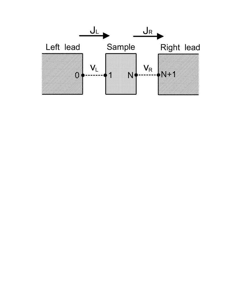
Fig.  1: Schematic picture of the system.

 

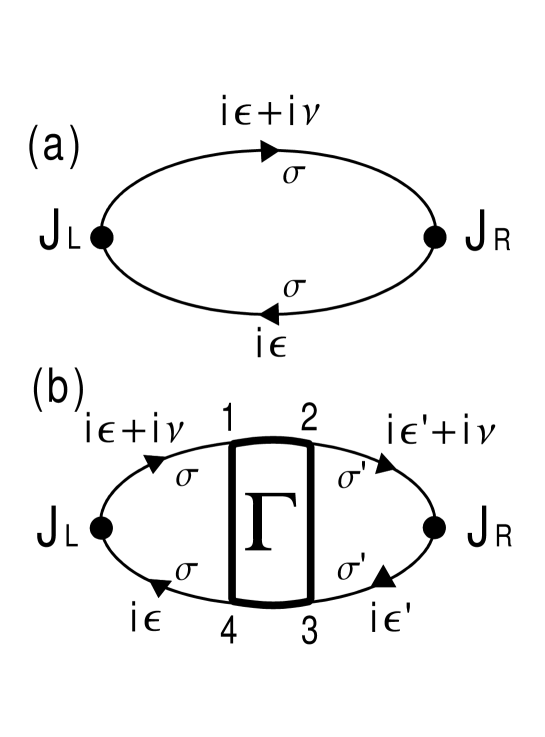
Fig.  2: Diagrams for $K_{RL}({\rm i}\nu)$. The shaded region represents the vertex part $\Gamma^{\sigma\sigma^{\prime}}_{12;\,34}({\rm i}\varepsilon,{\rm i}\varepsilon^{\prime};{\rm i}\nu)$.

 

Fig.  3: Three analytic regions of the current vertex $\Lambda_{R;j_{4}j_{1}}(z,z+w)$.

 

Fig.  4: Analytic regions of the vertex part $\Gamma^{\sigma\sigma^{\prime}}_{j_{1}j_{2};\,j_{3}j_{4}}(z,z^{\prime};w)$.

 

Fig.  5: Schematic picture of the model.

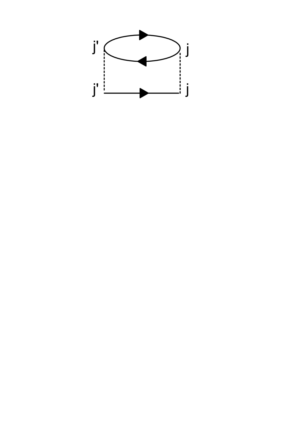
Fig.  6: The order $U^{2}$ self-energy $\Sigma_{jj^{\prime}}$.

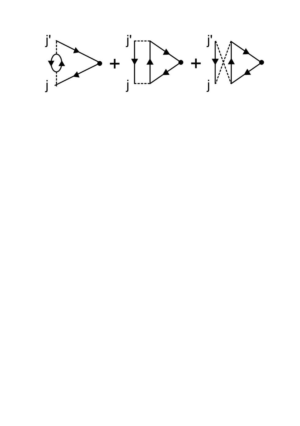
Fig.  7: The order $U^{2}$ current vertex $P_{jj^{\prime}}$.

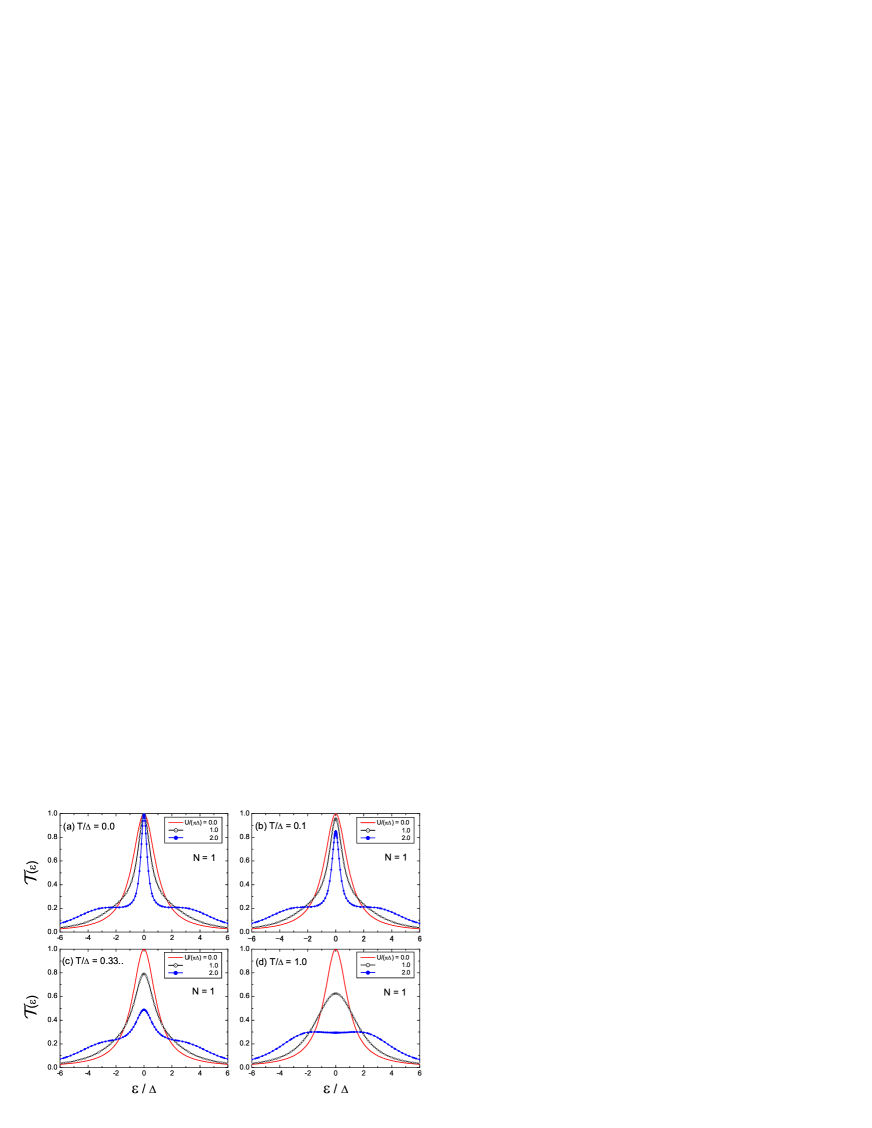
Fig.  8: Transmission probability for $N=1$. The temperature $T/\Delta$ is taken to be (a) $0.0$, (b) $0.1$, (c) $0.333\cdots$, and (d) $1.0$. The onsite interaction $U/(\pi\Delta)$ is taken to be (—) $0.0$, (–$\circ$–) $1.0$, and (–$\bullet$–) $2.0$. The horizontal axis $\epsilon$ is measured in units of $\Delta$ ($=2\Gamma$).

Fig.  9: Transmission probability for $N=2$. The temperature $T/t$ is taken to be (a) $0.0$, (b) $0.2$, (c) $0.333\cdots$, and (d) $0.5$. The onsite interaction $U/(2\pi t)$ is taken to be (—) $0.0$, (–$\circ$–) $0.5$, and (–$\bullet$–) $1.0$. The horizontal axis $\epsilon$ is measured in units of $t$. Here $\Gamma/t=0.75$.

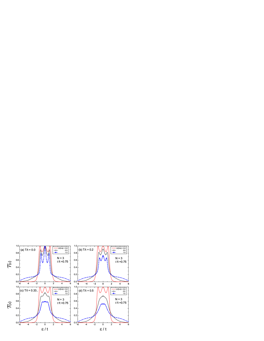
Fig.  10: Transmission probability for $N=3$. The temperature $T/t$ is taken to be (a) $0.0$, (b) $0.2$, (c) $0.333\cdots$, and (d) $0.5$. The onsite interaction $U/(2\pi t)$ is taken to be (—) $0.0$, (–$\circ$–) $0.5$, and (–$\bullet$–) $1.0$. The horizontal axis $\epsilon$ is measured in units of $t$. Here $\Gamma/t=0.75$.

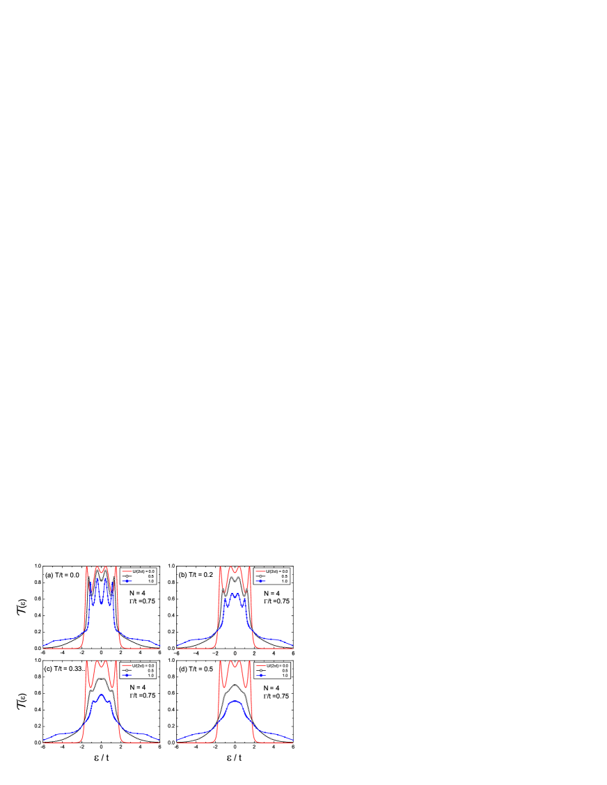
Fig.  11: Transmission probability for $N=4$. The temperature $T/t$ is taken to be (a) $0.0$, (b) $0.2$, (c) $0.333\cdots$, and (d) $0.5$. The onsite interaction $U/(2\pi t)$ is taken to be (—) $0.0$, (–$\circ$–) $0.5$, and (–$\bullet$–) $1.0$. The horizontal axis $\epsilon$ is measured in units of $t$. Here $\Gamma/t=0.75$.

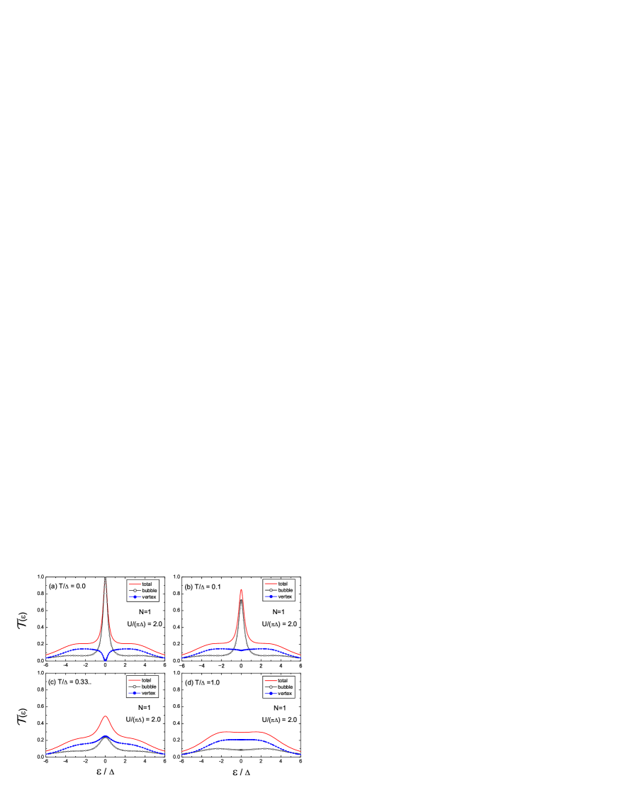
Fig.  12: The bubble ($\circ$) and vertex ($\bullet$) contributions to the transmission probability (solid line) for $N=1$. The temperature $T/\Delta$ is taken to be (a) $0.0$, (b) $0.1$, (c) $0.333\cdots$, and (d) $1.0$. Here $U/(\pi\Delta)=2.0$.

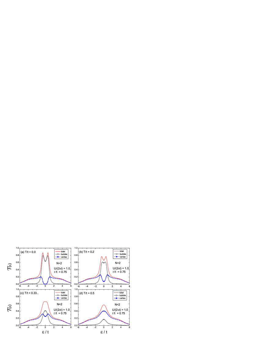
Fig.  13: The bubble ($\circ$) and vertex ($\bullet$) contributions to the transmission probability (solid line) for $N=2$. The temperature $T/t$ is taken to be (a) $0.0$, (b) $0.2$, (c) $0.333\cdots$, and (d) $0.5$. Here $U/(2\pi t)=1.0$, and $\Gamma/t=0.75$.

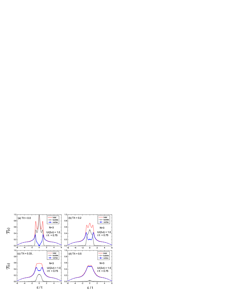
Fig.  14: The bubble ($\circ$) and vertex ($\bullet$) contributions to the transmission probability (solid line) for $N=3$. The temperature $T/t$ is taken to be (a) $0.0$, (b) $0.2$, (c) $0.333\cdots$, and (d) $0.5$. Here $U/(2\pi t)=1.0$, and $\Gamma/t=0.75$.

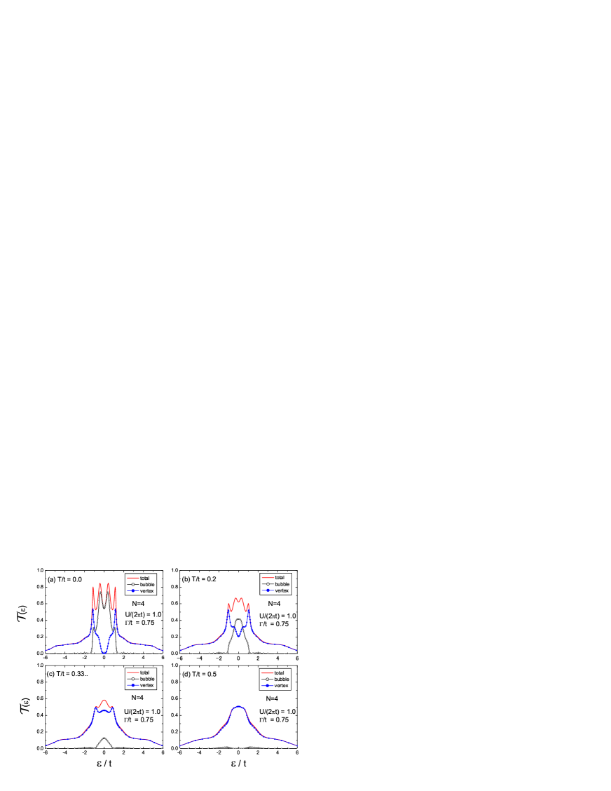
Fig.  15: The bubble ($\circ$) and vertex ($\bullet$) contributions to the transmission probability (solid line) for $N=4$. The temperature $T/t$ is taken to be (a) $0.0$, (b) $0.2$, (c) $0.333\cdots$, and (d) $0.5$. Here $U/(2\pi t)=1.0$, and $\Gamma/t=0.75$.

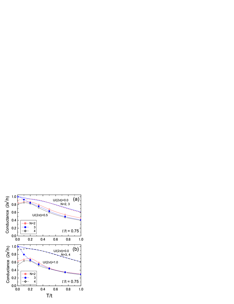
Fig.  16: Conductance vs temperature: $U/(2\pi t)$ is taken to be (a) $0.5$ and (b) $1.0$ for $N=2$ ($\Box$), $N=3$ ($\bullet$), and $N=4$ ($\Diamond$). The noninteracting results are also plotted for $N=2$ (dotted line), $N=3$ (solid line), and $N=4$ (dashed line). Here $\Gamma/t=0.75$.

References

- [1] A. C. Hewson: The Kondo Problem to Heavy Fermions (Cambridge University Press, Cambridge, 1993).
- [2] D. Goldharber-Gordon, H. Shtrikman, D. Mahalu, D. Abusch-Magder, U. Meirav, and M. A. Kastner: Nature 391 (1998) 156.
- [3] S. M. Cronenwett, T. H. Oosterkamp, and L. P. Kouwenhoven: Science 281 (1998) 540.
- [4] F. Simmel, R. H. Blick, J. P. Kotthaus, W. Wegscheider, and M. Bichler: Phys. Rev. Lett. 83 (1999) 804.
- [5] T. K. Ng and P. A. Lee: Phys. Rev. Lett. 61 (1988) 1768.
- [6] L. I. Glazman and M. E. Raikh: Pis’ma Zh. Eksp. Teor. Fiz. 47 (1988) 378 [JETP Lett. 47 (1988) 452].
- [7] A. Kawabata: J. Phys. Soc. Jpn. 60 (1991) 3222.
- [8] L. V. Keldysh: Zh. Eksp. Teor. Fiz. 47 (1964) 1515 [Sov. Phys. JETP 20 (1965) 1018].
- [9] C. Caroli, R. Combescot, P. Nozières, and D. Saint-James: J. Phys. C 4 (1971) 916.
- [10] Y. Meir and N. S. Wingreen: Phys. Rev. Lett. 68 (1992) 2512. The expression of the current has been shown to simplify in the case of in their notation.
- [11] A. Oguri: J. Phys. Soc. Jpn. 66 (1997) 1427.
- [12] A. Oguri: Phys. Rev. B 56 (1997) 13422; 58 (1998) 1690(E).
- [13] J. S. Langer and V. Ambegaokar: Phys. Rev. 121 (1961) 1090.
- [14] K. Yamada: Prog. Theor. Phys. 53 (1975) 970; Prog. Theor. Phys. 54 (1975) 316; K. Yosida and K. Yamada: Prog. Theor. Phys. 53 (1975) 1286.
- [15] H. Shiba: Prog. Theor. Phys. 54 (1975) 967.
- [16] A. Oguri: Phys. Rev. B 59 (1999) 12240.
- [17] A. Oguri: Phys. Rev. B 63 (2001) 115305.
- [18] G. M. Éliashberg: Zh. Eksp. Teor. Fiz. 41 (1961) 1241 [JETP 14 (1962) 886].
- [19] K. Yamada and K. Yosida: Prog. Theor. Phys. 76 (1986) 621.
- [20] R. Landauer: Philos. Mag. 21 (1970) 863.
- [21] M. Büttiker, Y. Imry, R. Landauer and S. Pinhas: Phys. Rev. B 31 (1985) 6207.
- [22] D. S. Fisher and P. A. Lee: Phys. Rev. B 23 (1981) 6851; P. A. Lee and D. S. Fisher: Phys. Rev. Lett. 47 (1981) 882.
- [23] W. Izumida and O. Sakai: Phys. Rev. B 62 (2000) 10260; J. Phys. Soc. Jpn. 70 (2001) 1045.
- [24] T. A. Costi: Phys. Rev. Lett. 85 (2000) 1504.
- [25] U. Gerland, J. von Delft, T. A. Costi, and Yuval Oreg: Phys. Rev. Lett. 84 (2000) 3710.
- [26] O. Sakai, S. Suzuki, W. Izumida, and A. Oguri: J. Phys. Soc. Jpn. 68 (1999) 1640.
- [27] S. Hersfield, J. H. Davies, and J. W. Wilkins: Phys. Rev. B 46 (1992) 7046.
- [28] A. Yeyati, A. Martín-Rodero, and F. Flores: Phys. Rev. Lett. 71 (1993) 2991.
- [29] T. Mii and K. Makoshi: Jpn. J. Appl. Phys. 35 (1996) 3706.
- [30] O. Takagi and T. Saso: J. Phys. Soc. Jpn. 68 (1999) 1997.
- [31] P. L. Pernas, F. Flores, and E. V. Anda: J. Phys. Cond. Matt. 4 (1992) 5309.
- [32] Y. Kawahito, H. Kasai, H. Nakanishi, and A. Okiji: J. Appl. Phys. 85 (1999) 947.
- [33] See, for instance, J. R. Schrieffer: Theory of Superconductivity (Benjamin, Massachusetts, 1964).
- [34] V. Horvatić, D. Šokčević, and V. Zlatić: Phys. Rev. B 36 (1987) 365.
- [35] T. A. Costi and A. C. Hewson: Physica 163 (1990) 179.
- [36] A. Oguri: unpublished.