Ferromagnetic transition in a double-exchange system with alloy disorder

Abstract

We study ferromagnetic transition in three-dimensional double-exchange model containing impurities. The influence of both spin fluctuations and impurity potential on conduction electrons is described in coherent potential approximation. In the framework of thermodynamic approach we construct Landau functional for the system ”electrons (in disordered environment) + core spins”. Analyzing the Landau functional we calculate the temperature of ferromagnetic transition $T_{C}$ and paramagnetic susceptibility $\chi$. For $T_{C}$, we thus extend the result obtained by Furukawa in the framework of the Dynamical Mean Field Approximation, with which our result coincides in the limit of zero impurity potential. We find, that the alloy disorder, able to produce a gap in density of electron states, can substantially decrease $T_{C}$ with respect to the case of no impurities. We also study the general relation between the Coherent Potential Approximation and the Dynamical Mean Field Approximation.

I Introduction

The recent rediscovery of colossal magnetoresistance in doped Mn oxides with perovskite structure R_1-xD_xMnO₃ (R is a rare-earth metal and D is a divalent metal, typically Ba, Sr or Ca) [1] substantially increased interest in the double-exchange (DE) model [2, 3]. Several approaches were used lately to study the thermodynamic properties of the DE model, including the Dynamical Mean Field Approximation (DMFA) [4] (and references therein; DMFA itself see [5]), Green functions decoupling techniques [6], Schwinger bosons [7], variational mean-field approach [8] and numerical methods [9, 10, 11]. In all these approaches chemical disorder introduced by doping, which is generic for the manganites, has not been taken into account.

Recently we have shown that the concurrent action of the chemical and magnetic disorder, is crucial for the the description of the density of states and conductivity in manganites [12]. In the present paper we consider the ferromagnetic transition in the case of non-zero potential of randomly distributed impurities, using the same coherent potential approximation (CPA) [13, 14, 15] as in our previous paper [12] (see also relevant Ref.[16]). Briefly, the effect of impurities on the transition is the reduction of $T_{C}$ as the impurity potential strength increases. In more detail, at values of the impurity potential at which the electron band is split off into two sub-bands, the mechanism of ferromagnetic exchange is other than in the case of the zero or weak potential.

II Hamiltonian and CPA equations

We consider the DE model with the inclusion of the single-site impurity potential. We apply the quasiclassical adiabatic approximation and consider each core spin as a static vector of fixed length $S$ (${\bf S}_{i}=S{\bf n}_{i}$, where ${\bf n}_{i}$ is a unit vector). The Hamiltonian of the model $H([{\bf n}_{i}])$ in site representation is

$$\hat{H}_{ij}=t_{i-j}+\left(\epsilon_{i}-J{\bf n}_{i}\cdot\hat{\bf\sigma}\right)\delta_{ij},$$ (1)

where $t_{i-j}$ is the electron hopping, $\epsilon_{i}$ is the on-site energy, $J$ is the effective exchange coupling between a core spin and a conduction electron and $\hat{\bf\sigma}$ is the vector of the Pauli matrices. The hat above the operator reminds that it is a $2\times 2$ matrix in the spin space (we discard the hat when the operator is a scalar matrix in the spin space). The Hamiltonian (1) is random due to randomness of a core spin configuration $[{\bf n}_{j}]$ and the randomness of the on-site energies $\epsilon_{i}$.

To handle CPA we present Hamiltonian (1) as

$$\hat{H}=\overbrace{\left(t_{i-j}+\hat{\Sigma}\delta_{ij}\right)}^{\hat{H}^{0}}+\overbrace{\left(\epsilon_{i}-J{\bf n}_{i}\cdot\hat{\bf\sigma}-\hat{\Sigma}\right)\delta_{ij}}^{\hat{V}}$$ (2)

(the site independent self-energy $\hat{\Sigma}(E)$ is to be determined later), and construct a perturbation theory with respect to random potential $\hat{V}$. To do this let us introduce the exact $T$-matrix as the solution of the equation

$$\hat{T}=\hat{V}+\hat{V}\hat{G}_{0}\hat{T},$$ (3)

in which $\hat{G}_{0}=(E-\hat{H}^{0})^{-1}$. For the exact Green function $\hat{G}$ we get

$$\hat{G}=\hat{G}_{0}+\hat{G}_{0}\hat{T}\hat{G}_{0}.$$ (4)

The self energy is determined from the requirement

$$\left\langle\hat{G}\right\rangle_{{\bf n},\epsilon}=\hat{G}_{0}$$ (5)

where the angular brackets with the indexes mean averaging over the configurations of both core spins and impurities. In CPA $\hat{T}$ is considered in a single-site approximation, at which Eq. (5) is reduced to the equation

$$\left\langle\hat{T}_{i}\right\rangle_{{\bf n},\epsilon}=0,$$ (6)

where $\hat{T}_{i}$ is the solution of the equation

$$\hat{T}_{i}=\hat{V}_{i}+\hat{V}_{i}\hat{g}(E)\hat{T}_{i}.$$ (7)

Here

$$\hat{g}(E)=g_{0}(E-\hat{\Sigma}),$$ (8)

$$g_{0}(E)=\int_{-\infty}^{\infty}\frac{N_{0}(\varepsilon)}{E-\varepsilon}d\varepsilon,$$ (9)

$N_{0}(\varepsilon)$ being the bare (i.e. for $\epsilon_{i}=0$ and $J=0$) density of states (DOS). Finally Eq. (6) can be transformed to an algebraic equation for the $2\times 2$ matrix $\hat{\Sigma}$:

$$\hat{g}=\left\langle\left(\hat{\Sigma}+\hat{g}^{-1}-\hat{V}_{i}\right)^{-1}\right\rangle_{{\bf n},\epsilon}.$$ (10)

III Band structure

To consider the evolution of the DOS

$$N(E)=\frac{1}{\pi}\mbox{Im}\;g_{c},$$ (11)

where $g_{c}=\mbox{Tr}\;\hat{g}$ (here Tr means the trace over spin states only), with the variation of the impurity concentration and potential strength, we exploit the semi-circular (SC) bare DOS given at $\left|\varepsilon\right|\leq W$ ($W$ is half of the bandwidth) by

$$N_{0}(\varepsilon)=\frac{2}{\pi W}\sqrt{1-\left(\frac{\varepsilon}{W}\right)^{2}},\;$$ (12)

and equal to zero otherwise. For this DOS (which is exact on a Caley tree)

$$g_{0}(E)=\frac{2}{W}\left[\frac{E}{W}-\sqrt{\left(\frac{E}{W}\right)^{2}-1}\right].$$ (13)

Hence we obtain

$$\hat{\Sigma}=E-2w\hat{g}-\hat{g}^{-1},$$ (14)

where $w=W^{2}/8$. Thus, Eq. (10) transforms to

$$\hat{g}=\left\langle\left(E-\epsilon+J{\bf n}{\bf\sigma}-2w{\hat{g}}\right)^{-1}\right\rangle_{{\bf n},\epsilon}.$$ (15)

It is convenient to write the locator $\hat{g}$ in the form

$$\hat{g}=\frac{1}{2}(g_{c}\hat{I}+{\bf g}_{s}\hat{{\bf\sigma}}),$$ (16)

where $\hat{I}$ is a unity matrix. For the charge locator $g_{c}$ and spin locator ${\bf g}_{s}$ we obtain the system of equations

$$g_{c}=2\left\langle\frac{E-\epsilon-wg_{c}}{\left(E-\epsilon-wg_{c}\right)^{2}-(J{\bf n}-w{\bf g}_{s})^{2}}\right\rangle_{{\bf n},\epsilon}$$ (17)

$${\bf g}_{s}=2\left\langle\frac{w{\bf g}_{s}-J{\bf n}}{\left(E-\epsilon-wg_{c}\right)^{2}-(J{\bf n}-w{\bf g}_{s})^{2}}\right\rangle_{{\bf n},\epsilon}.$$ (18)

In the strong Hund coupling limit ($J\rightarrow\infty$) we obtain from Eqs. (17) two decoupled spin sub-bands. For the lower sub-band, after shifting the energy by $J$ we obtain

$$g_{c}=\left\langle\frac{1}{E-\epsilon-wg_{c}-wn^{z}g_{s}}\right\rangle_{{\bf n},\epsilon}$$ (19)

$$g_{s}=\left\langle\frac{n^{z}}{E-\epsilon-wg_{c}-wn^{z}g_{s}}\right\rangle_{{\bf n},\epsilon},$$ (20)

where ${\bf g}_{s}=(0,0,g_{s})$ an axis OZ is directed along the average magnetization of core spins ${\bf m}$).

In fact, details of alloying define how to average over the configurations of impurities in Eqs. (17,19). We use for this random substitution model of disorder. That is $\epsilon_{i}=V$ with the probability $x$ and $\epsilon_{i}=0$ with the probability $1-x$, where $V$ and $x$ are the impurity potential and concentration, respectively. As to core spins, once CPA is introduced, their configuration probability should be determined self-consistently in order to close Eqs. (17,19). In the Appendix we prove that in the presence of an annealed disorder (including dynamical one) DMFA ansatz for the disorder configuration probability [5] keeps the free energy stationary against variations of CPA $\hat{\Sigma}$.

For the following two cases, however, only the averaging over $\epsilon$ is left. For a saturated ferromagnetic (FM) phase ($m=1$), we obtain $g_{s}=g_{c}$, and closed equation for the charge locator is

$$g_{c}=\left\langle\frac{1}{E-\epsilon-2wg_{c}}\right\rangle_{\epsilon},$$ (21)

For a paramagnetic (PM) phase ($m=0$), we obtain ${\bf g}_{s}=0$, and closed equation for the charge locator is

$$g_{c}^{(0)}=\left\langle\frac{1}{E-\epsilon-wg_{c}^{(0)}}\right\rangle_{\epsilon}.$$ (22)

It appears that calculation of $g_{c}^{(0)}$ is sufficient for obtaining $T_{C}$ and the PM susceptibility $\chi$ as functions of $x$ and $V$.

The results of numerical calculation of the DOS at the PM state are presented on Fig. 1 (specific $x$ and different $V$).

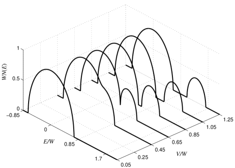
FIG. 1.: The calculated DOS as function of the relative strength of impurity potential $V/W$ for $x=0.18$.

and on Fig. 2 (specific $V$ and different $x$).

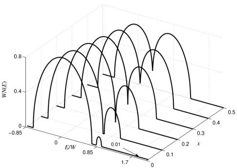
FIG. 2.: The calculated DOS as function of impurity concentration $x$ for $V/W=0.69$.

When comparing Eqs. (21) and (22) it is seen that the DOS in the FM phase is equal to the DOS in the PM state of another model, with increased by a factor of $\sqrt{2}$ bare bandwidth. Using this property and Fig. 1 we conclude that at an appropriate $V/W$ there may be a gap between the conduction band states and the impurity band states in the PM phase, while the FM DOS is gapless. This may explain metal-insulator transition observed in manganites and magnetic semiconductors [12]. It is also seen from Fig. 2 that the gap in the DOS existing at low concentrations may close at higher concentrations. The value of the impurity potential $V_{c}=W/\sqrt{2}$ detaches two types of the gap behavior. At $V<V_{c}$ the gap opens for some $x<0.5$ or does not open at all, at $V>V_{c}$ the gap exists for all $0<x\leq 0.5$, and at $V=V_{c}$ the gap closes exactly for $x=0.5$. Anyhow, even if the gap is closed there still may exist pseudogap at a strong enough potential (see Fig. 2).

The dependence of the gap $\Delta$ on $x$ at several $V/W$ is shown on on Fig. 3, which summarizes the regularities discussed above.

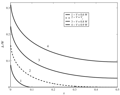
FIG. 3.: The calculated gap in the DOS as function of impurity concentration $x$ at different strengths of impurity potential $V$.

It is worth noting, that at $V>V_{c}$, $\Delta$ is near to saturate after $x>0.25$. This may explain the near independence of the resistivity activation energy on $x$ in the PM phase observed in single crystalline manganites [17] (the fact used by some authors to support the polaron scenarios of the transport at $T>T_{C}$).

IV Landau functional

In our approach the calculation of thermodynamic properties is based on the analysis of the Landau functional. We start from the exact partition function of the system electrons + core spins

$$Z=\int\exp\left[-\beta\Omega([{\bf n}_{j}])+\beta{\bf H}\cdot\sum_{i=1}^{N}{\bf n}_{i}\right]\prod_{i=1}^{N}d{\bf n}_{j},$$ (23)

where $N$ is the number of core spins, ${\bf H}$ is magnetic field, $\beta=1/T$, and $\Omega([{\bf n}_{j}])$ is the grand canonical potential of the electron subsystem for a given core spin configuration $[{\bf n}_{j}]$. Our aim is to obtain Landau functional of the system.

Since we use CPA for electronic properties it is consistent to construct the Landau functional using a mean-field approach. Mean-field means that we do not take into account large-scale fluctuations of the macroscopic magnetization ${\bf M}=\frac{1}{N}\sum_{j}{\bf n}_{j}$, but within CPA we certainly take into account microscopic fluctuations of ${\bf n}_{i}$. In the mean-field approximation all energy levels depend only upon ${\bf M}$. Hence we may approximately put

$$\Omega([{\bf n}_{j}])\approx\Omega(M),$$ (24)

where $\Omega(m)$ is the grand canonical potential calculated within CPA at a non-zero ${\bf m}$. Then the partition function can be written as

$$Z=\int\exp\left[-\beta L({\bf M},{\bf H})\right]d{\bf M},$$ (25)

where

$$L({\bf M},{\bf H})=\Omega(M)-N{\bf H}\cdot{\bf M}-TS(M);$$ (26)

the quantity

$$S(M)=\ln\int\delta\left({\bf M}-\frac{1}{N}\sum_{i=1}^{N}{\bf n}_{i}\right)\prod_{i=1}^{N}d{\bf n}_{j}$$ (27)

is the entropy of the core spin subsystem. So we may identify the functional $L({\bf M},{\bf H})$ in the exponent of Eq. (25) with the Landau functional of the whole system [18].

At high temperatures the minimum of $L({\bf M},0)$ is at $M=0$. At low temperatures the point $M=0$ corresponds to the maximum of this functional. Let us expand $L({\bf M},0)$ with respect to $M$

$$L({\bf M},0)=L_{0}(T)-L_{2}(T)M^{2}+\mbox{O}\;(M^{4}),$$ (28)

$$L_{2}(T)=\Omega_{2}(T)-TS_{2}.$$ (29)

Here the coefficients are defined from the the second-order expansions of $S(M)$

$$S(M)=S_{0}-S_{2}M^{2}+\dots,$$ (30)

where $S_{2}=\frac{2}{3}N$ [18], and of $\Omega(m)$

$$\Omega(m)=\Omega_{0}(T)-\Omega_{2}(T)m^{2}+\dots$$ (31)

which is to be constructed. Thus the critical temperature $T_{C}$, below which the functional has the minimum at some $M\neq 0$, is defined from the equation

$$L_{2}(T_{C})=\Omega_{2}(T_{C})-T_{C}S_{2}=0.$$ (32)

The magnetic susceptibility in the PM phase is given by the equation

$$\frac{2}{N}\chi(T)=\frac{1}{TS_{2}-\Omega_{2}(T)}.$$ (33)

The grand canonical potential of the electron subsystem is given by

$$\Omega(m)=-\frac{N}{\pi\beta}\int_{-\infty}^{+\infty}\ln\left[1+e^{-\beta(E-\mu)}\right]N(E)dE,$$ (34)

where $N(E)$ is the DOS given by Eq. (11) and $\mu$ is the chemical potential determined from the equation

$$n=\int_{-\infty}^{+\infty}f(E,\mu)N(E)dE,$$ (35)

in which $f(E,\mu)$ is the Fermi function and $n=1-x$ is the number of electrons per site.

V Calculation of $T_{c}$ and $\chi(T)$

Due to the constancy of $n$ (or $x$) the calculation of $\Omega_{2}(T)$ requires only the second-order expansion of $N(E)$ with respect to $m$, which is obtained via Eq. (11) thus expanding Eq. (19)

$$g_{c}=g_{c}^{(0)}+g_{c}^{(2)}m^{2}+\dots,$$ (36)

Substituting the related result for $N^{(2)}(E)$ into Eqs. (34), (32) and (33) , we obtain the following equations

$$T_{C}=\Theta(T_{C},\mu(T_{C})),$$ (37)

$$\frac{3}{N}\chi(T)=\frac{1}{T-\Theta(T,\mu(T))}$$ (38)

In these equations $\mu(T)$ is determined from Eq. (35) where $N(E)$ is replaced by its PM value $N^{(0)}(E)$, and

$$\Theta(T,\mu)=\frac{2w}{3\pi\beta}\int_{-\infty}^{\infty}\ln\left[1+e^{-\beta(E-\mu)}\right]$$ (39)

$$\mbox{Im}\left\{\frac{\left\langle g_{\epsilon}\right\rangle_{\epsilon}\left[\left\langle g_{\epsilon}^{2}\right\rangle_{\epsilon}+\frac{w}{3}\left(\left\langle g_{\epsilon}\right\rangle_{\epsilon}\left\langle g_{\epsilon}^{3}\right\rangle_{\epsilon}-\left\langle g_{\epsilon}^{2}\right\rangle_{\epsilon}^{2}\right)\right]}{(1-w\left\langle g_{\epsilon}^{2}\right\rangle_{\epsilon})\left(1-\frac{w}{3}\left\langle g_{\epsilon}^{2}\right\rangle_{\epsilon}\right)^{2}}\right\}dE,$$ (40)

where

$$g_{\epsilon}=\frac{1}{E-\epsilon-wg_{c}^{(0)}},$$ (41)

Using Eq. (22) and integrating by parts, we obtain

$$\Theta(T,\mu)=\int_{-\infty}^{\infty}f(E,\mu)\theta(E)dE,$$ (42)

where

$$\theta(E)=-\frac{w}{3\pi}\mbox{Im}\left\{\frac{\left\langle g_{\epsilon}\right\rangle_{\epsilon}^{2}}{1-\frac{w}{3}\left\langle g_{\epsilon}^{2}\right\rangle_{\epsilon}}\right\},$$ (43)

The function $\theta(E)$ being integrated with respect to energy gives exactly zero. This leads to $T_{C}(x)=T_{C}(1-x)$, which reflects the particle-hole symmetry of our model irrespective of the disorder strength.

In the case where the DOS is smooth, the inequality $W\gg T_{C}$ allows us to consider electrons as nearly degenerate. In this case both $\mu$ and $\Theta(T,\mu)$ do not depend upon $T$, and Eq. (37) is just a ready formula for $T_{C}$. The same is true if there is developed gap. In this case $\mu$ is near the middle of the gap, so we can substitute $f(E,\mu)$ by one, provided that the integration in Eq. (42) extends only over the filled sub-band. In both these cases $\chi(T)$ obeys the Curie-Weiss law (see Eq. (38)). In the first case the ferromagnetic order is mediated mostly by mobile holes that is specific for DE. In the second case the concentration of the mobile carriers (both holes and electrons) is exponentially small. So effective exchange between core spins is mostly due to virtual transitions of electrons from the lower filled to the upper empty sub-band via the gap. This mechanism is an analog of super-exchange (SE) acting in the system with electron disorder.

If $\Delta\sim T$ or there is a pseudogap with a strong dip in the DOS, the integration in Eqs. (35) and (42) should take into account the tails of $f(E,\mu)$. The exchange in such cases is intermediate between DE and SE types.

For the case of no on-site disorder our Eq. (37) for $T_{C}$ coincides with Eq. (49) of Ref. [19], obtained in the framework of DMFA and calculated numerically versus $x$. In this case we even managed to calculate the integral in Eq. (42) analytically, to get for $T_{C}$:

$$T_{C}=\frac{W\sqrt{2}}{4\pi}\left[\sqrt{1-y^{2}}-\frac{1}{\sqrt{3}}\tan^{-1}\sqrt{3(1-y^{2})}\right],$$ (44)

$$y=\sqrt{2}\mu/W,$$ (45)

while Eq. (35) takes the form

$$x=\frac{1}{2}-\frac{1}{\pi}\left(\sin^{-1}y+y\sqrt{1-y^{2}}\right).$$ (46)

When the disorder is taken into account the integration in Eq. (42)-(37) is done numerically. The results for $T_{C}(x)$ at different $V/W$ are presented on Fig. 4. The upper (dashed) curve calculated at $V=0$ is the same as plotted using Eqs. (44)-(46)

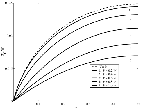
FIG. 4.: The calculated Curie temperature as function of $x$ at different $V/W$.

One notices that the increase of the impurity potential leads to progressive decrease of $T_{C}$. This decrease becomes more substantial at $V/W$ and $x$ able to produce the gap in the density of states. This trend marks the modification of the ferromagnetic exchange mechanism which accompanies the electron band splitting. As in the case of DE alone $T_{C}$ still increases from zero to a maximum value upon increasing $x$ from $x=0$ to $x=0.5$.

VI Discussion

Our results show that $T_{C}$ is decreased by the presence of impurities with strong enough potential. It may be questioned in this connection why low value of $T_{C}$ in manganites would be on account of fluctuations beyond DMFA in the pure DE model rather than due to the alloy disorder. The present study reveals an interesting, though hardly experimentally detectable, feature - the alternation of ferromagnetic exchange mechanism from DE to SE like as the impurity band splits off the conduction band.

A Dynamical Mean Field Approximation for General Strongly Correlated System

In most interesting cases the partition function of a strongly correlated electron system may be represented as functional integral

$$Z=\int Z\left[v,{\mathbf{h}}\right]\prod_{i}P_{v}\left[v_{i}\right]P_{{\mathbf{h}}}\left[{\mathbf{h}}_{i}\right]{\mathcal{D}}v_{i}\left(\tau\right){\mathcal{D}}{\mathbf{h}}_{i}\left(\tau\right)$$ (A1)

in which the integrand $Z\left[v,{\mathbf{h}}\right]$ is the partition function of non-interacting electrons system posed in imaginary-time $\tau$ and site $i$ dependent potential $v_{i}\left(\tau\right)$ and magnetic ${\mathbf{h}}_{i}\left(\tau\right)$ fields distributed independently on different sites with on-site probability densities $P_{v}\left[v\right]$ and $P_{{\mathbf{h}}}\left[{\mathbf{h}}\right]$, respectively. The free-electron partition function is represented by the integral

$$Z\left[v,{\mathbf{h}}\right]=\int\exp\left\{\int_{0}^{\beta}\overline{\psi}\cdot\left[\frac{\partial}{\partial\tau}+\mu-{\mathcal{H}}\left(\tau\right)\right]\cdot\psi\right\}{\mathcal{D}}\overline{\psi}{\mathcal{D}}\psi$$ (A2)

over anticommuting fields $\psi=\left\{\psi_{i\alpha}\right\}$ and its conjugate $\overline{\psi}$, where the imaginary-time $\tau$ dependent Hamiltonian ${\mathcal{H}}\left(\tau\right)$ is defined by the matrix elements

$${\mathcal{H}}_{i\alpha,j\beta}\left(\tau\right)=t_{i\alpha,j\beta}+v_{i\alpha,j\beta}\left(\tau\right);$$ (A3)

$$t_{i\alpha,j\beta}=t\left(i-j\right)\delta_{\alpha,\beta},\,v_{i\alpha,j\beta}\left(\tau\right)=V_{\alpha\beta}\left(i;\tau\right)\delta_{i,j}$$ (A4)

$$V_{\alpha\beta}\left(i;\tau\right)=v_{i}\left(\tau\right)\delta_{\alpha,\beta}-{\mathbf{h}}_{i}\left(\tau\right)\cdot{\mathbf{\sigma}}_{\alpha\beta}$$ (A5)

(the electron charge and magneton are absorbed in the corresponding fields). The Grassmanian integral in Eq. (A2) is calculated in the familiar form

$$Z\left[v,{\mathbf{h}}\right] = \mbox{Det}{\mathcal{G}}^{-1}=\exp\left\{-S\left[v,{\mathbf{h}}\right]\right\}$$ (A6)

$$S\left[v,{\mathbf{h}}\right] = \log\mbox{Det}{\mathcal{G}}=\mbox{Tr}{}\log{\mathcal{G}}$$ (A7)

where ${\mathcal{G}}^{-1}=\frac{\partial}{\partial\tau}+\mu-{\mathcal{H}}$; the matrix element of ${\mathcal{G}}$ with respect to site, spin and imaginary time, ${\mathcal{G}}_{i\alpha,j\beta}\left(\tau,\tau^{\prime}\right)$, is the fermionic Green-Matsubara kernel satisfying the equation

$$\left(\frac{\partial}{\partial\tau}+\mu\right){\mathcal{G}}_{i\alpha,j\beta}\left(\tau,\tau^{\prime}\right)$$ (A8)

$$-\sum_{k,\gamma}{\mathcal{H}}_{i\alpha,k\gamma}\left(\tau\right){\mathcal{G}}_{k\gamma,j\beta}\left(\tau,\tau^{\prime}\right)={\mathcal{I}}_{i\alpha,j\beta}\left(\tau,\tau^{\prime}\right)$$ (A9)

where

$${\mathcal{I}}_{i\alpha,j\beta}\left(\tau,\tau^{\prime}\right)=\delta_{i,j}\delta_{\alpha,\beta}\delta\left(\tau-\tau^{\prime}\right)$$ (A10)

is the unity matrix. Thus we obtain for the partition function

$$Z=\int\prod_{i}P_{v}\left[v_{i}\right]P_{{\mathbf{h}}}\left[{\mathbf{h}}_{i}\right]\exp\left\{-S\left[v,{\mathbf{h}}\right]\right\}{\mathcal{D}}v_{i}\left(\tau\right){\mathcal{D}}{\mathbf{h}}_{i}\left(\tau\right)$$ (A11)

and for the number of electrons

$$N_{e}=\frac{1}{\beta}\frac{\partial}{\partial\mu}\log Z=\frac{1}{\beta}\left\langle\mbox{Tr}{}{\mathcal{G}}\right\rangle_{v,{\mathbf{h}}}$$ (A12)

(which is the equation for chemical potential $\mu$) where the average of every functional $\Phi=\Phi\left[v,{\mathbf{h}}\right]$ is defined by

$$\left\langle\Phi\right\rangle_{v,{\mathbf{h}}}=\frac{1}{Z}\int\prod_{i}P_{v}\left[v_{i}\right]P_{{\mathbf{h}}}\left[{\mathbf{h}}_{i}\right]$$ (A13)

$$\exp\left\{-S\left[v,{\mathbf{h}}\right]\right\}\Phi\left[v,{\mathbf{h}}\right]{\mathcal{D}}v_{i}\left(\tau\right){\mathcal{D}}{\mathbf{h}}_{i}\left(\tau\right)$$ (A14)

Assume that, in addition to ’annealed’ disorder described by $v_{i}\left(\tau\right)$ and ${\mathbf{h}}_{i}\left(\tau\right)$, there exists a ’quenched’ disorder described by independently fluctuating static on-site energies $\epsilon_{i}$. Then the fields $v_{i}\left(\tau\right)$ in the Hamiltonian are to be replaced by $v_{i}\left(\tau\right)+\epsilon_{i}$ and the observables should be additionally averaged over given distribution of the quenched disorder. For example, free energy is given by

$$F=\left\langle-\frac{1}{\beta}\log Z\right\rangle_{\epsilon}+\mu N_{e}=\frac{1}{\beta}\left\langle-\log Z+\mu\mbox{Tr}\left\langle{}{\mathcal{G}}\right\rangle_{v,{\mathbf{h}}}\right\rangle_{\epsilon}$$ (A15)

Consider an effective medium described by the bare hopping Hamiltonian $t$ plus some self-energy given by translationally invariant and stationary matrix $\Sigma_{\alpha\beta}\left(i-j,\tau-\tau^{\prime}\right)$. The Green-Matsubara kernel for such a medium is also translationally invariant and stationary: $\overline{{\mathcal{G}}}_{i\alpha,j\beta}\left(\tau,\tau^{\prime}\right)=$ $\overline{{\mathcal{G}}}_{\alpha\beta}\left(i-j,\tau-\tau^{\prime}\right)$, and can be expressed via Fourier transform

$$\overline{{\mathcal{G}}}\left({\mathbf{k}},i\omega_{m}\right)=\left[i\omega_{m}+\mu-t\left({\mathbf{k}}\right)-\Sigma\left({\mathbf{k}},i\omega_{m}\right)\right]^{-1}$$ (A16)

where $\omega_{m}$ is the Matsubara frequency, $\Sigma_{\alpha\beta}\left({\mathbf{k}},i\omega_{m}\right)$ is Fourier transform of $\Sigma_{\alpha\beta}\left(i-j,\tau-\tau^{\prime}\right)$ and the quantities in both sides of Eq. (A16) are matrices in spin space. From the very meaning of effective medium it is to be required

$$\overline{{\mathcal{G}}}=\left\langle\left\langle{\mathcal{G}}\right\rangle_{v,{\mathbf{h}}}\right\rangle_{\epsilon}$$ (A17)

that implicitly defines the self-energy. Eq. (A17) can be transformed to another form using $T$-Matrix ansatz for the exact Green-Matsubara kernel. We have

$${\mathcal{G}}=\overline{{\mathcal{G}}}+\overline{{\mathcal{G}}}{\mathcal{T}}\overline{{\mathcal{G}}}$$ (A18)

where ${\mathcal{T}}$ is the exact $T$-Matrix

$${\mathcal{T}}=\left({\mathcal{I}}-{\mathcal{V}}\overline{{\mathcal{G}}}\right)^{-1}{\mathcal{V}}$$ (A19)

where ${\mathcal{V}}$ is the effective interaction with the matrix elements

$${\mathcal{V}}_{i\alpha,j\beta}\left(\tau,\tau^{\prime}\right)=v_{i\alpha,j\beta}\left(\tau\right)\delta\left(\tau-\tau^{\prime}\right)-s_{i\alpha,j\beta}\left(\tau,\tau^{\prime}\right)$$ (A20)

(Note that the effective interaction unlike true one is non-local). Then Eq. (A17) is exactly equivalent to following equation

$$\left\langle\left\langle{\mathcal{T}}\right\rangle_{v,{\mathbf{h}}}\right\rangle_{\epsilon}=0$$ (A21)

which expresses the requirement of zero scattering on average. It can easily be understood that the complexity of solving Eq. (A21) to determine $\Sigma_{\alpha\beta}\left(i-j,\tau-\tau^{\prime}\right)$ or $\Sigma_{\alpha\beta}\left({\mathbf{k}},i\omega_{m}\right)$ is the same as that of calculating ${\mathcal{G}}$ at every disorder configuration and then performing the average. To develop a working approximation let us apply the idea of Coherent Potential Approximation (CPA) (used exceptionally for quenched disorder) to the present case. Within CPA one firstly puts

$$\Sigma_{\alpha\beta}\left(i-j,\tau-\tau^{\prime}\right)=\delta_{i,j}\Sigma_{\alpha\beta}\left(\tau-\tau^{\prime}\right)$$ (A22)

$$\Sigma\left({\mathbf{k}},i\omega_{m}\right)=\Sigma\left(i\omega_{m}\right)$$ (A23)

(so ${\mathcal{V}}$ becomes also local in space) and secondly applies the zero-order locality approximation

$$\overline{{\mathcal{G}}}_{\alpha\beta}\left(i-j,\tau-\tau^{\prime}\right)\simeq g_{\alpha\beta}\left(\tau-\tau^{\prime}\right)\delta_{i,j}$$ (A24)

$$g_{\alpha\beta}\left(\tau\right)=\overline{{\mathcal{G}}}_{\alpha\beta}\left(0,\tau\right)$$ (A25)

to the term ${\mathcal{V}}\overline{{\mathcal{G}}}$ in Eq. (A19). This leads to approximate space locality of the transfer matrix as follows

$${\mathcal{T}}_{i\alpha,j\beta}\left(\tau,\tau^{\prime}\right)\approx T_{\alpha\beta}\left(i;\tau,\tau^{\prime}\right)\delta_{i,j}$$ (A26)

where the elements of the local transfer matrix $\hat{T}_{i}$ satisfy the integral equation

$$T_{\alpha\beta}\left(i;\tau,\tau^{{}^{\prime}}\right)-\int_{0}^{\beta}\left[V_{\alpha\gamma}\left(i;\tau\right)\delta\left(\tau-\upsilon\right)\right.$$ (A27)

$$\left.-\Sigma_{\alpha\gamma}\left(\tau-\upsilon\right)\right]g_{\gamma\delta}\left(\upsilon-\upsilon^{\prime}\right)T_{\delta\beta}\left(i;\upsilon,\upsilon^{\prime}\right)d\upsilon d\upsilon^{\prime}$$ (A28)

$$=V_{\alpha\beta}\left(i;\tau\right)\delta\left(\tau-\tau^{{}^{\prime}}\right)-\Sigma_{\alpha\beta}\left(\tau-\tau^{{}^{\prime}}\right)$$ (A29)

The relaxed form of Eq. (A21), which is essentially CPA equation, reads

$$\left\langle\left\langle\hat{T}_{i}\right\rangle_{v,{\mathbf{h}}}\right\rangle_{\epsilon}=0$$ (A30)

We use symbolic solution of Eq. (A29)

$$\hat{T}_{i}=\left[\hat{I}-\left(\hat{V}_{i}-\hat{\Sigma}\right)\hat{g}\right]^{-1}\left(\hat{V}_{i}-\hat{\Sigma}\right),$$ (A31)

where $\hat{I}$, $\hat{V}_{i}$, $\hat{\Sigma}$ and $\hat{g}$ are the matrices with the elements $\delta_{\alpha\beta}\delta\left(\tau-\tau^{{}^{\prime}}\right)$, $V_{\alpha\beta}\left(i;\tau\right)\delta\left(\tau-\tau^{{}^{\prime}}\right)$, $\Sigma_{\alpha\beta}\left(\tau-\tau^{{}^{\prime}}\right)$ and $g_{\alpha\beta}\left(\tau-\tau^{{}^{\prime}}\right)$ respectively. Hence one may rearrange Eq. (A30) to the form

$$\hat{g}=\left\langle\left\langle\left(\hat{g}^{-1}+\hat{\Sigma}-\hat{V}_{i}\right)^{-1}\right\rangle_{v,{\mathbf{h}}}\right\rangle_{\epsilon}.$$ (A32)

There arises a question of how to consistently perform average over $v$ and ${\mathbf{h}}$ in Eqs.(A30),(A32), which may sound strange because the answer seems ready. Indeed, upon the approximation given by Eq. (A26) and the exact decomposition given by Eq. (A18) one gets the approximate expression for ${\mathcal{G}}$ which would be used to calculate the approximate entropy functional due to Eq. (A7):

$$S\left[v,{\mathbf{h}}\right]\simeq\log\mbox{Det}\overline{{\mathcal{G}}}+\log\mbox{Det}\left({\mathcal{I}}+T\overline{{\mathcal{G}}}\right)$$ (A33)

However this expression is still too cumbersome to be used for averaging since $\overline{{\mathcal{G}}}$ has intersite matrix elements, neglected when solving for ${\mathcal{T}}$ (it concerns only the second term because the first doesn’t depend on random fields). But if we again apply the approximation of Eq. (A25), this time to the term $T\overline{{\mathcal{G}}}$, and make use of Eqs. (A31), (A32) we obtain just site-additive entropy functional

$$S\left[v,{\mathbf{h}}\right]\simeq\mbox{Tr}\log\overline{{\mathcal{G}}}+\sum_{i}s_{i}\left[v_{i},{\mathbf{h}}_{i}\right],$$ (A34)

$$s_{i}\left[v_{i},{\mathbf{h}}_{i}\right]=\log\det\left(\hat{I}+\hat{T}_{i}\hat{g}\right)$$ (A35)

where ’tr’ and ’det’ mean corresponding operations only with respect to spin and $\tau$ variables. The admission of $S\left[v,{\mathbf{h}}\right]$ in the form of Eq. (A35) is just Dynamical Mean Field Approximation (DMFA) ansatz. Let us show that DMFA is the best in variational sense, consistent with CPA, approximation, namely that it ensures the stationarity of the approximate free energy

$$F_{a}=\beta^{-1}\left(\mbox{Tr}\log\overline{{\mathcal{G}}}+\mu\mbox{Tr}{}\overline{{\mathcal{G}}}\right)-$$ (A36)

$$\beta^{-1}\sum_{i}\left\langle\log\int\exp\left\{-s_{i}\left[v_{i},{\mathbf{h}}_{i}\right]\right\}\right.$$ (A37)

$$\left.P_{v}\left[v_{i}\right]P_{{\mathbf{h}}}\left[{\mathbf{h}}_{i}\right]{\mathcal{D}}v_{i}\left(\tau\right){\mathcal{D}}{\mathbf{h}}_{i}\left(\tau\right)\right\rangle_{\epsilon}$$ (A38)

with respect to any variations of the local self-energy. To prove this let us first note that variation of the first two terms in brackets on account of varying $\mu$ cancels out. So we obtain upon variation of the matrix $\hat{\Sigma}$

$$\beta\delta F_{a}=\sum_{i}\mbox{tr}\left\{\left(\delta\hat{g}^{-1}+\delta\hat{\Sigma}\right)\right.$$ (A39)

$$\left.\left[\hat{g}-\left\langle\left\langle\left(\hat{g}^{-1}+\hat{\Sigma}-\hat{V}_{i}\right)^{-1}\right\rangle_{v,{\mathbf{h}}}\right\rangle_{\epsilon}\right]\right\}$$ (A40)

where $\delta\hat{g}^{-1}$is the variation of the matrix $\hat{g}^{-1}$ due to the variation of $\hat{\Sigma}$. Now it is seen that for the stationarity, that is $\delta F_{a}=0$, it is necessary and sufficient satisfying Eq. (A32) or equivalent Eq. (A30).

B Double Exchange Model with Classical Core Spins

In the case of DE Model considered we have $v_{i}\left(\tau\right)=0$ and static magnetic fields

$${\mathbf{h}}_{i}\left(\tau\right)=J{\mathbf{n}}_{i}.$$ (B1)

So

$$P_{{\mathbf{h}}}[{\mathbf{h}}_{i}{\mathbf{]}}=\delta\left({\mathbf{n}}_{i}^{2}-1\right)$$ (B2)

In present case we can use Fourier transform with respect to $\tau$. We obtain the basic equations

$$g\left(i\omega_{m}\right)=\left\langle\frac{\int\frac{\exp\left\{-s\left[\epsilon,{\mathbf{n}}\right]\right\}}{\hat{g}^{-1}\left(i\omega_{m}\right)+\hat{\Sigma}\left(i\omega_{m}\right)-\epsilon+J{\mathbf{n}}\cdot{\mathbf{\hat{}}{\sigma}}}d{\mathbf{n}}}{\int\exp{\left\{-s\left[\epsilon,{\mathbf{n}}\right]\right\}}d{\mathbf{n}}}\right\rangle_{\epsilon}$$ (B3)

where

$$s\left[\epsilon,{\mathbf{n}}\right]=\sum_{\omega_{n}}\log\det\left\{\hat{I}+\left[\hat{\Sigma}\left(i\omega_{n}\right)-\epsilon+J{\mathbf{n}}\cdot{\mathbf{\hat{}}{\sigma}}\right]\hat{g}\left(i\omega_{n}\right)\right\}^{-1},$$ (B4)

and

$$\hat{g}\left(i\omega_{m}\right)=\int N_{0}\left(\varepsilon\right)\left[i\omega_{m}+\mu-\varepsilon-\hat{\Sigma}\left(i\omega_{m}\right)\right]^{-1}d\varepsilon.$$ (B5)

REFERENCES

• [1] R. von Helmolt et al., Phys. Rev. Lett. 71, 2331 (1993); K. Chadra et al., Appl. Phys. Lett. 63, 1990 (1993); S. Jin et al., Science 264, 413 (1994).
• [2] C. Zener, Phys. Rev. 82, 403 (1951).
• [3] P. W. Anderson and H. Hasegawa, Phys. Rev. 100, 675 (1955).
• [4] N. Furukawa: in Physics of Manganites, ed. T. Kaplan and S. Mahanti (Plenum Publishing, New York, 1999).
• [5] A. Georges, G. Kotliar, W. Krauth, and M. J. Rozenberg, Rev. Mod. Phys. 68, 13 (1996).
• [6] A. C. M. Green and D. M. Edwards, J. Phys.: Cond. Matt. bf 11, 10511 (1999).
• [7] D. P. Arovas, G. Gomes-Santos, F. Guinea, Phys.Β Rev.Β B59, 13569 (1999); F. Guinea, G. Gomes-Santos, D. P. Arovas, Phys.Β Rev.Β B62, 391 (2000).
• [8] J. L. Alonso, L. A. Fernandez, F. Guinea, V. Laliena, and V. Martin-Mayor, Phys. Rev. B 63, 054411 (2001).
• [9] S. Yunoki, J. Hu, A. L. Malvezzi, A. Moreo, N. Furukawa, and E. Dagotto, Phys.Β Rev.Β Lett.80, 845 (1998).
• [10] Y. Motome and N. Furukawa, J. Phys. Soc. Jpn. 69, 3785 (2000).
• [11] H. RΓΆder, R. R. P. Singh, and J. Zang, Phys.Β Rev.Β B56, 5084 (1997).
• [12] M. Auslender and E. Kogan, Eur. Phys. J. B, 19, 525 (2001); cond-mat/0102469.
• [13] J. M. Ziman, Models of Disorder, Cambridge University Press, 1979.
• [14] P. Soven, Phys. Rev. 156, 809 (1967); D. Taylor, Phys. Rev. 156, 1017 (1967).
• [15] A. Rangette, A. Yanase, and J. Kubler, Solid State Comm. 12, 171 (1973); K. Kubo, J. Phys. Soc. Japan 36, 32 (1974).
• [16] B. M. Letfulov and J. K. Freericks, cond-mat/0103471. This paper treats the subject using a model in which only Ising-like part of electron core spin exchange is retained; such model lacks O(3) symmetry inherent to DE model.
• [17] A. P. Ramirez, J. Phys.: Cond. Matt. 9, 8171 (1997).
• [18] J. F. Negele and H. Orland, Quantum Many-Particle Systems (Perseus Books, Reading MA, 1998).
• [19] N. Furukawa, cond-mat/9812066.