Nature of the spin-glass state in the three-dimensional gauge glass

Abstract

We present results from simulations of the gauge glass model in three dimensions using the parallel tempering Monte Carlo technique. Critical fluctuations should not affect the data since we equilibrate down to low temperatures, for moderate sizes. Our results are qualitatively consistent with earlier work on the three- and four-dimensional Edwards-Anderson Ising spin-glass. We find that large scale excitations cost only a finite amount of energy in the thermodynamic limit, and that those excitations have a surface whose fractal dimension is less than the space dimension, consistent with a scenario proposed by Krzakala and Martin, and Palassini and Young.

]

I Introduction

The ground state structure of spin-glasses is poorly understood. While there has been considerable work on Ising-type spin-glass systems[1, 2, 3, 4], models with a vector order parameter symmetry have not yet been analyzed in much detail. Here we study the three-dimensional gauge glass since it is a simple model with a vector order parameter in which a finite-temperature spin-glass transition[5] has been well established.

There are two theories describing the spin-glass phase: the “droplet picture” (DP) by Fisher and Huse[6] and the replica symmetry breaking picture (RSB) by Parisi[7, 8]. According to the droplet picture, a cluster of spins of size $L$ costs an energy proportional to $L^{\theta}$ where $\theta$ is positive. This implies that, in the thermodynamic limit, excitations which flip a finite cluster of spins cost an infinite energy. In addition, these excitations have a fractal surface with a fractal dimension $d_{s}$ that is smaller than the space dimension $d$. By contrast, RSB follows the exact solution of the Sherrington-Kirkpatrick model in predicting that there are excitations which turn over a finite fraction of the spins and which cost a finite amount of energy in the thermodynamic limit. The surface of these excitations is space filling[3], i.e. $d_{s}=d$. Another difference between these models can be quantified by looking at the distribution of the order parameter[3, 9, 10, 11] $P(q)$. In the droplet picture, according to the standard interpretation[12, 13], $P(q)$ is trivial, i.e. there are only two peaks at $\pm q_{\rm EA}$in the thermodynamic limit ($q_{\rm EA}$ the Edwards-Anderson order parameter). For finite systems of linear size $L$, there is a tail with weight $\sim L^{-\theta}$ down to $q=0$. On the contrary, RSB predicts also a tail with a finite weight down to $q=0$ independent of system size.

Recently, there have been results by Krzakala and Martin[1], as well as Palassini and Young[2] (referred to as KMPY) for Ising-type systems that find an intermediate picture: while large scale excitations cost only a finite amount of energy in the thermodynamic limit, their surface is fractal with $d_{s}<d$. In this scenario, it is necessary to introduce two exponents, $\theta$ and $\theta^{\prime}$, to describe the system size dependence of the excitation energy, where $L^{\theta}$ is the typical energy of an excitation of size $L$ induced by a change in boundary conditions, and $\theta^{\prime}$ describes the size dependence of the energy of clusters thermally excited at fixed boundary conditions.

In this paper we test which of the above predictions apply to the gauge glass by performing Monte Carlo simulations down to low temperatures for a modest range of sizes using the parallel tempering Monte Carlo method[14, 15], as previously done in Ref. [4] for the three- and four-dimensional Edwards-Anderson Ising spin-glass. We find that $P(0)$ does not decrease with increasing system size and, from data for $q_{l}$, we deduce that $d_{s}<d$, consistent with the existence of KMPY excitations.

The layout of the paper is as follows: In Sec. II we describe the model as well as the observables measured while in Sec. III we discuss our equilibration tests for the parallel tempering Monte Carlo method. Our results are discussed in Sec. IV. In Sec. V we summarize our conclusions and present some ideas for future work.

II Model and Observables

The Hamiltonian of the gauge glass is given by

$${\cal H}=-J\sum_{\langle i,j\rangle}\cos(\phi_{i}-\phi_{j}-A_{ij}),$$ (1)

where the sum ranges over nearest neighbors on a square lattice in three dimensions of size $N=L\times L\times L$ and $\phi_{i}$ represent the angles of the XY spins. Periodic boundary conditions are applied. $J$ is a positive ferromagnetic coupling between nearest neighbor spins and $A_{ij}$ represents the line integral of the vector potential directed from site $i$ to site $j$,

$$A_{ij}=\frac{2\pi}{\Phi_{0}}\int_{{\bf r}_{i}}^{{\bf r}_{j}}{\bf A}\cdot d{\bf l},$$ (2)

and $\Phi_{0}=hc/(2e)$ is the flux quantum. The $A_{ij}$ are quenched random variables uniformly distributed between $[0,2\pi]$. In this work we set $J=1$. Note that on average the gauge glass is isotropic even though there are local quenched fluxes.

This model is often used to describe disordered high-$T_{c}$ superconductors[16] in a magnetic field since, even though it lacks screening, it has the right order parameter symmetry.

The order parameter of the gauge glass is traditionally defined as

$$Q={1\over N}\sum_{i=1}^{N}[\langle e^{i\phi_{i}}\rangle^{\prime}\langle e^{-i\phi_{i}}\rangle^{\prime}]_{\rm av},$$ (3)

where we indicate thermal averages by angular brackets, $\langle\ldots\rangle$, and averages of over the disorder by rectangular brackets, $[\ldots]_{\rm av}$. If we average over all possible global rotations of the spins then the thermal averages in Eq. (3) vanish, so we need to work in an ensemble where global rotations of are not permitted (e.g. by applying a small symmetry breaking field along the $\phi=0$ direction) for Eq. (3) to be sensible. This is indicated by the prime on the thermal average. In the simulation we evaluate the product of the two thermal averages by simulating two copies (replicas) of the system with the same quenched disorder, and so Eq. (3) becomes

$$Q=[\langle\,q\,\rangle^{\prime}]_{\rm av},$$ (4)

where the microscopic spin overlap $q$ is defined by

$$q=\frac{1}{N}\sum_{j=1}^{N}\exp\left(i(\phi^{\alpha}_{i}-\phi^{\beta}_{i})\right),$$ (5)

where $\alpha$ and $\beta$ refer to the two replicas. In the constrained ensemble, if we write $q\,(\equiv q_{x}+iq_{y})$ in terms of its real and imaginary parts, then $\langle q_{y}\rangle^{\prime}=0$ and $\langle q\rangle^{\prime}=\langle q_{x}\rangle^{\prime}$.

In practice it is inconvenient to constrain the ensemble by applying a symmetry breaking field, so instead we perform a rotation of one replica relative to the other in order to maximize $q_{x}$ (and simultaneously set $q_{y}$ to zero). It is easy to see that $q_{x}$ in the rotated frame is just $|q|$ (which is invariant under rotations). We therefore take the spin order parameter to be $|q|$ and its expectation value to be

$$Q=[\langle\,|q|\,\rangle],$$ (6)

(no prime now indicating an unconstrained thermal average) which is to be compared with Eq. (4). In the unconstrained ensemble, the probability to get particular values for $q_{x},q_{y}$ only depends on $|q|$.

In addition, we will also study the link overlap $q_{l}$, defined by

$$q_{l}=\frac{1}{N_{b}}\sum_{\langle i,j\rangle}\cos\left((\phi_{i}^{\alpha}-\phi_{i}^{\beta})-(\phi_{j}^{\alpha}-\phi_{j}^{\beta})\right),$$ (7)

where $N_{b}=Nd$ is the number of bonds ($d=3$ is the space dimension). The sum ranges over all nearest-neighbor pairs of spins. Note that while a change in $q$ induced by flipping a cluster of spins is proportional to the volume of the cluster, $q_{l}$ changes by an amount promotional to the surface of the cluster.

The weight in $P(\left|q\right|)$ for small $|q|$ varies as $L^{-\theta^{\prime}}$, where $\theta^{\prime}$ was introduced in section I. In addition we expect the variance of the link overlap to fit to a form ${\rm Var}(q_{l})\sim L^{-\mu_{l}}$ where, as shown in Ref. [4], $\mu_{l}=\theta^{\prime}+2(d-d_{s})$.

III Equilibration

For the simulations we use the parallel tempering Monte Carlo method[14, 15] as it allows us to study larger systems at lower temperatures. In this technique, one simulates several identical replicas of the system at different temperatures, and, in addition to the usual local moves, one performs global moves in which the temperatures of two replicas (with adjacent temperatures) are exchanged. This method does not allow us to use the equilibration test first introduced by Bhatt and Young[17] because the system temperature does not stay constant throughout the simulation. The equilibration test for short range spin-glasses simulated with parallel tempering Monte Carlo introduced in Ref. [4] by Katzgraber et. al does not work here either because the disorder is not Gaussian. To ensure that the system is equilibrated, we therefore require that different moments of $q$ and $q_{l}$ are independent of the number of Monte Carlo steps $N_{\mathrm{sweep}}$. Figure 1 shows data for several moments of $q$ and $q_{l}$ as a function of Monte Carlo Steps. One can clearly see that the different moments saturate at the same equilibration time. Here we show data for an intermediate size ($L=4$) since we can better illustrate the procedure by calculating longer equilibration times. We also require the acceptance ratios of the moves which interchange temperatures to be at least $0.3$ or higher and roughly constant as a function of temperature.

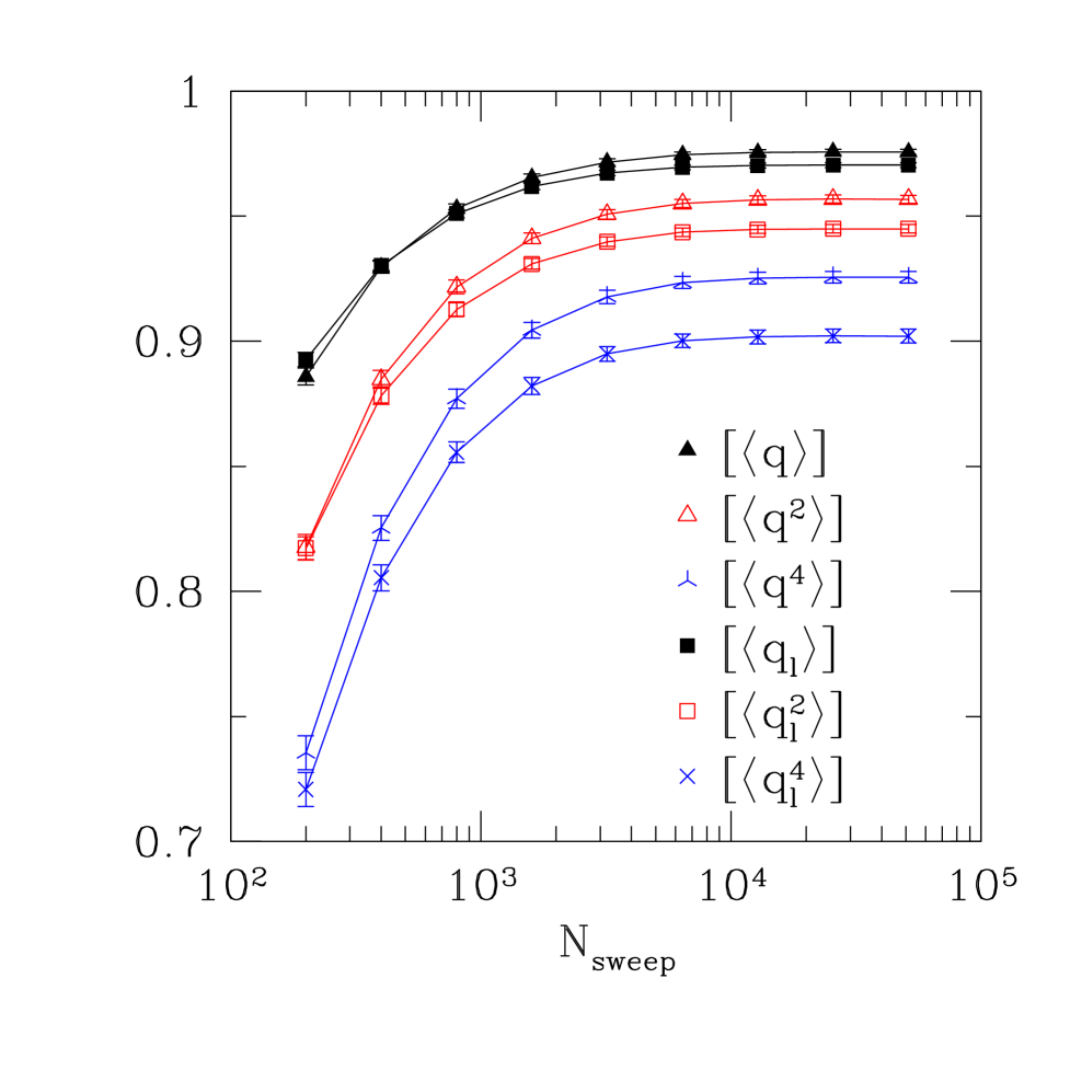
FIG. 1.: Moments of the overlap and link overlap, defined by Eqs. (5) and (7) respectively, as a function of Monte Carlo sweeps $N_{\mathrm{sweep}}$, that each of the replicas perform, averaged over the last half of the sweeps. Note that the moments seem to equilibrate roughly at the same time and appear to be independent of the number of sweeps. The data shown is for $L=4$ and $T=0.050$, the lowest temperature studied.

As another test for equilibration, we require the distribution of $q_{x},q_{y}$, which we call $P_{xy}(q_{x},q_{y})$, to be symmetric about the origin. Figure 2 shows a density plot of $P_{xy}(q_{x},q_{y})$ for $L=4$ at different temperatures. We see clearly that the distributions do not depend on the angle from the origin, as required.

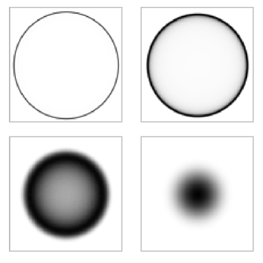
FIG. 2.: Two-dimensional density plots of $P_{xy}(q_{x},q_{y})$ vs. $q_{x}$, $q_{y}$ for $L=4$. The horizontal (vertical) axis represents $q_{x}$ ($q_{y}$). Dark corresponds to a region of high probability. Note that for different temperatures ranging from below to above $T_{c}$ the distributions are symmetric around $q=0$. (Clockwise from top left: $T=$ 0.050, 0.166, 0.520 and 0.947).

In Table I, we show $N_{\mathrm{samp}}$ (number of samples), $N_{\mathrm{sweep}}$ (total number of sweeps performed by each set of spins), and $N_{T}$ (number of temperature values), used in the simulations. For each size, the largest temperature is 0.947 and the lowest temperature is 0.050. This is to be compared with[5, 18] $T_{c}\approx 0.45$. The set of temperatures is determined by requiring that the acceptance ratios for moves which exchange temperatures are satisfactory for the largest size, $L=8$, and for simplicity the same temperatures also are used for the smaller sizes. We also want the distribution of $q$ at the highest temperature to show a Gaussian shape centered at $q=0$ to ensure that all free-energy barriers have vanished so the system will randomize quickly. The lower-right image for $T=0.947\gg T_{c}$ in Figure 2 shows this is the case. For all system sizes, the acceptance ratios for global moves are always greater than 0.3 for each pair of temperatures.

$L$	$N_{\mathrm{samp}}$	$N_{\mathrm{sweep}}$	$N_{T}$
3	$1.0\times 10^{4}$	$6.0\times 10^{3}$	53
4	$1.0\times 10^{4}$	$2.0\times 10^{4}$	53
5	$1.0\times 10^{4}$	$6.0\times 10^{4}$	53
6	$5.0\times 10^{3}$	$2.0\times 10^{5}$	53
8	$2.0\times 10^{3}$	$1.2\times 10^{6}$	53

TABLE I.: Parameters of the simulations. $N_{\mathrm{samp}}$ is the number of samples, i.e. sets of gauge fields, $N_{\mathrm{sweep}}$ is the total number of sweeps simulated for each of the $2N_{T}$ replicas for a single sample, and $N_{T}$ is the number of temperatures used in the parallel tempering method.

Since the gauge glass has a vector order parameter symmetry, to speed up the simulation we discretize the angles of the spins to $N_{\phi}=512$. This number is large enough to avoid any crossover effects to other models as discussed by Cieplak et. al[19]. To ensure a reasonable acceptance ratio for single-spin Monte Carlo moves, we pick the proposed new angle for a spin within an acceptance window about the current angle, where the size of the window is proportional to the temperature $T$. By tuning a numerical prefactor we ensure the acceptance ratios for these local moves are not smaller than 0.2 for each system size at the lowest temperature simulated.

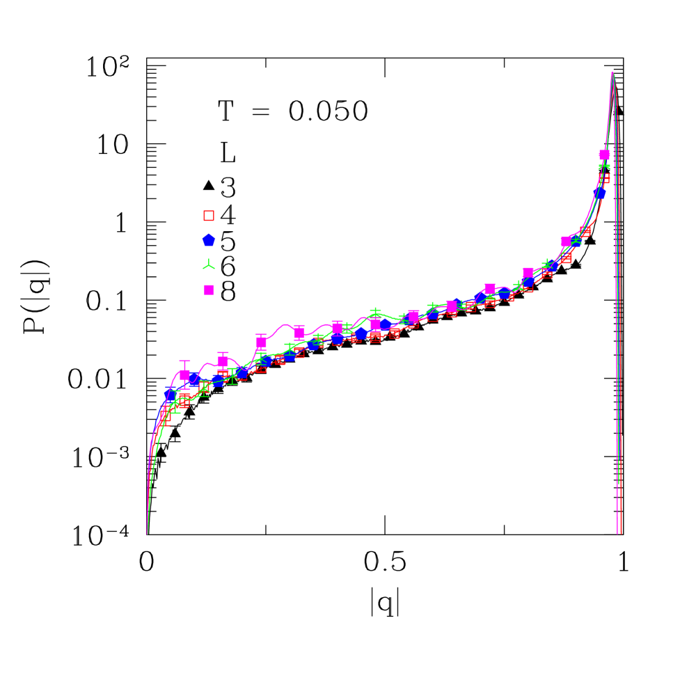
FIG. 3.: Data for the overlap distribution $P(\left|q\right|)$ at temperature $T=0.050$ for different system sizes. Note the logarithmic vertical scale. In this and other similar figures in the paper, we only display a subset of all the data points while the lines connect all the data points in the set. Thus, the wiggles in the lines between neighboring symbols are meaningful.

IV Results

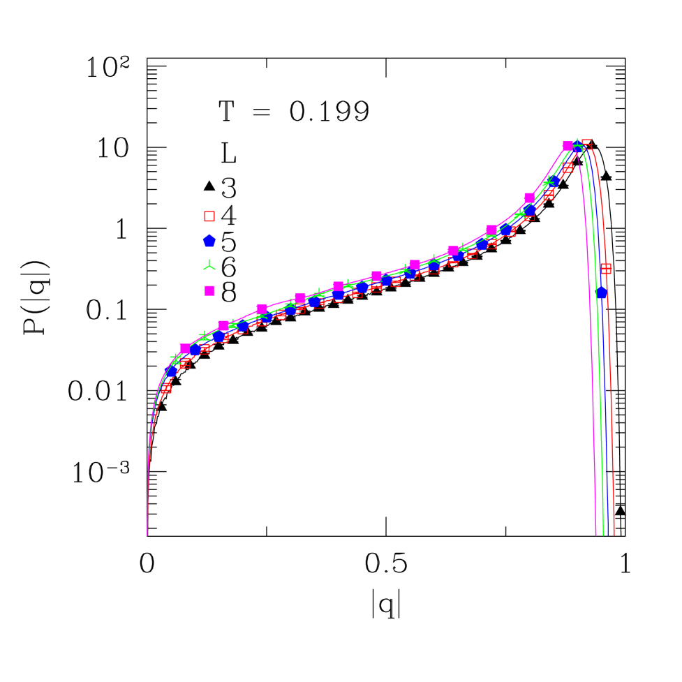
FIG. 4.: Same as Figure 3 but at temperature $T=0.199$.

Figures 3 and 4 show data for $P(\left|q\right|)$ at $T=0.050$ and $0.199$, well below[5] $T_{c}\approx 0.45$. There is a clear peak for large $\left|q\right|$ as well as a tail at small $\left|q\right|$. The weight in the tail does not decrease with increasing $L$, as would be expected in the standard interpretations of the droplet theory. If anything, the weight actually increases somewhat for larger sizes.

Note that $P(\left|q\right|)$ decreases to zero, linearly, at very small $\left|q\right|$. This is clearly a phase space factor, since the the two-dimensional probability distribution $P_{xy}(q_{x},q_{y})$, plotted in Figure 2, will not diverge for a finite system, and $P(\left|q\right|)=2\pi\left|q\right|P_{xy}(q_{x},q_{y})$. In order to have $P(\left|q\right|)$ tend to a constant for $\left|q\right|\to 0$, a prediction of RSB, the region of $\left|q\right|$ over which $P(\left|q\right|)$ drops linearly must tend to zero for $L\to\infty$, and also $P_{xy}(q_{x},q_{y})$ must diverge as $1/\left|q\right|$ in this limit. There is some evidence, particularly from Figure 3, that $P(\left|q\right|)$ stays flat down to smaller $\left|q\right|$ for larger $L$, though the range of sizes is too small to make a reliable extrapolation.

Figures 5 and 6 show data for $P(q_{l})$. As with the distributions of $\left|q\right|$, there is a pronounced peak at large $q_{l}$-values. The width of the distribution decreases with increasing system size.

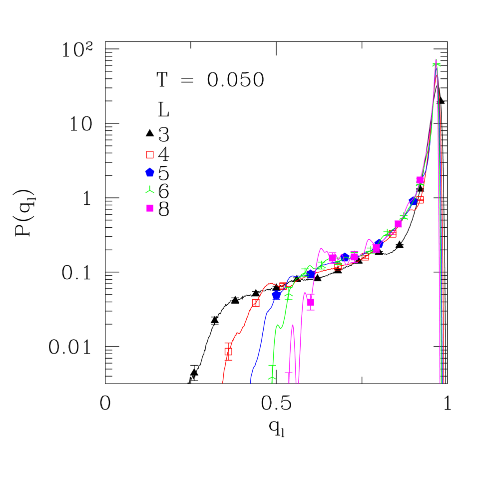
FIG. 5.: The distribution of the link overlap at $T=0.050$ for different sizes. Note the logarithmic vertical scale.

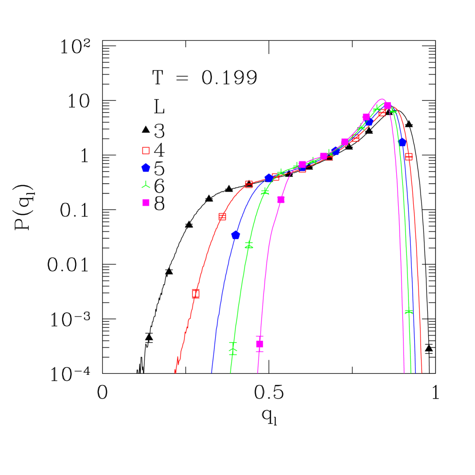
FIG. 6.: Same as Figure 5 but at temperature $T=0.199$.

The variance of $P(q_{l})$ is shown in Figure 7 for several low temperatures. The data is consistent with a power law decrease where the (presumably effective) exponent varies slightly with $T$. Extrapolating to $T=0$ gives $\mu_{l}\equiv\theta^{\prime}+2(d-d_{s})=0.501\pm 0.04$. Assuming $\theta^{\prime}\approx 0$ we find

$$d-d_{s}=0.25\pm 0.02,$$ (8)

implying that system-size excitations have a fractal surface in the thermodynamic limit as predicted by the droplet picture.

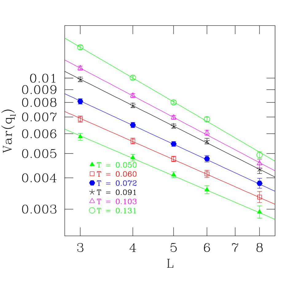
FIG. 7.: Log-log plot of the variance of $q_{l}$ as a function of system size $L$ at several temperatures.

V Conclusions

To conclude, Monte Carlo simulations of the three-dimensional gauge glass at low temperatures show that the structure of the spin-glass state in this particular model agrees qualitatively with previous results for Ising spin-glasses[4] and is in agreement with the KMPY picture. From the non-trivial form of $P(q)$ for a modest range of sizes we infer that system-size excitations cost a finite amount of energy in the thermodynamic limit. From the variance of the link overlap it appears that the surface of these excitations is fractal with $d-d_{s}=0.25\pm 0.02$. Work is in progress on other vector spin-glass models to see if they have the same features found here and for the Ising spin-glass.

These results, however, involve a large extrapolation to the thermodynamic limit. There may exist a crossover length at larger sizes to a different behavior such as the droplet theory or an RSB picture.

- [1] F. Krzakala and O. C. Martin, Phys. Rev. Lett. 85, 3013 (2000).
- [2] M. Palassini and A. P. Young, Phys. Rev. Lett. 85, 3017 (2000).
- [3] E. Marinari, G. Parisi, F. Ricci-Tersenghi, J. Ruiz-Lorenzo and F. Zuliani, J. Stat. Phys. 98, 973 (2000).
- [4] H. G. Katzgraber, M. Palassini and A. P. Young, Phys. Rev. B 63, 184422, (2001).
- [5] T. Olson and A. P. Young, Phys. Rev. B 61, 12467 (2000).
- [6] D. S. Fisher and D. A. Huse, J. Phys. A. 20 L997 (1987); D. A. Huse and D. S. Fisher, J. Phys. A. 20 L1005 (1987); D. S. Fisher and D. A. Huse, Phys. Rev. B 38 386 (1988).
- [7] G. Parisi, Phys. Rev. Lett. 43, 1754 (1979); J. Phys. A 13, 1101, 1887, L115 (1980; Phys. Rev. Lett. 50, 1946 (1983).
- [8] M. Mézard, G. Parisi and M. A. Virasoro, Spin glass Theory and Beyond (World Scientific, Singapore, 1987).
- [9] J. D. Reger, R. N. Bhatt and A. P. Young, Phys. Rev. Lett. 64, 1859 (1990).
- [10] E. Marinari, G. Parisi, and J. J. Ruiz-Lorenzo, in Spin glasses and Random Fields, edited by A. P. Young (World Scientific, Singapore, 1998), and references therein.
- [11] E. Marinari and F. Zuliani, J. Phys. A 32, 7447 (1999).
- [12] A. J. Bray and M. A. Moore, in Heidelberg Colloquium on Glassy Dynamics and Optimization, edited by L. Van Hemmen and I. Morgenstern (Springer-Verlag, Berlin, 1986), p. 121.
- [13] M. A. Moore, H. Bokil, and B. Drossel, Physical Review Letters 81, 4252 (1998).
- [14] K. Hukushima and K. Nemoto, J. Phys. Soc. Japan 65, 1604 (1996).
- [15] E. Marinari, Advances in Computer Simulation, edited by J. Kertész and I. Kondor (Springer-Verlag, Berlin 1998), p. 50, (cond-mat/9612010).
- [16] For a review of vortices in superconductors, see G. Blatter, M. V. Feigel’man, V. B. Geshkenbein, A. I. Larkin and V. M. Vinokur, Rev. Mod. Phys. 66, 1125 (1994).
- [17] R. N. Bhatt and A. P. Young, Phys. Rev. Lett. 54, 924 (1985); ibid., Phys. Rev. B 37, 5606 (1988).
- [18] J. D. Reger, T. A. Tokuyasu, A. P. Young and M. P. A. Fisher, Phys. Rev. B 44, 7147 (1991).
- [19] M. Cieplak, J. .R. Banavar, M. S. Li and A. Khurana, Phys. Rev. B 45, 786 (1992).