MICROSCOPIC MODELS FOR LONG RANGED VOLATILITY CORRELATIONS

Abstract

We propose a general interpretation for long-range correlation effects in the activity and volatility of financial markets. This interpretation is based on the fact that the choice between ‘active’ and ‘inactive’ strategies is subordinated to random-walk like processes. We numerically demonstrate our scenario in the framework of simplified market models, such as the Minority Game model with an inactive strategy, or a more sophisticated version that includes some price dynamics. We show that real market data can be surprisingly well accounted for by these simple models.

1 Introduction

When looking at the time series of the daily returns in liquids markets, it appears to the naked eye that the observed behaviour is markedly non Gaussian: fluctuations are intermittent and strong, localized outbursts of volatility can be identified. This fact, known as volatility clustering [1, 2, 3], can be analyzed more quantitatively by looking at the daily volatility $\sigma_{t}$ (defined for example, as the average squared high frequency return). This quantity follows a log-normal distribution [5], and its temporal correlation function $\langle\sigma_{t}\sigma_{t+\tau}\rangle$ can be fitted by an inverse power of the lag $\tau$, with a rather small exponent in the range $0.1-0.3$ [1, 4, 5, 6]. This suggests that there is no characteristic time scale for volatility fluctuations: outbursts of market activity can persist for rather short times (say a few days), but also for much longer times, months or even years. Besides, these long ranged volatility correlations are observed on many different financial markets and over different periods of time, with qualitatively similar features: stocks, currencies, commodities or interest rates (see for example the bund contract discussed in [3]). This suggests that a common mechanism is at the origin of this rather universal phenomenon. This universality, which is also observed for other ‘stylized facts’ of financial markets (for example the power law behaviour of the return distribution) has attracted much attention, especially among physicists. It indeed supports the idea of the market as a complex interacting system of the kind usually studied in physics, where complex behaviour arises from individual actions, not crucially depending on the details of the microscopic interactions.

In this line of thought, the approach of agent based modelling has been intensively pursued, and important insights into market dynamics have recently been gained [8, 10, 11, 12, 13, 14, 15, 16, 17, 18]. These models postulate some simple behaviour at the level of the agents and investigate the resulting price dynamics. Their aim is to reproduce real market phenomenology and understand its distinctive features in terms of microscopic mechanisms. Of course the possibilities of modelling are a priori numerous, since very little is known about the relevant ingredients needed to construct a realistic artificial market. In this context two possible strategies of investigation can be followed. The first is to look for very simple models, which may be in some respects unrealistic, but where both analytical resolution and intuitive understanding can be reached. Alternatively, one can focus on more complex models, trying to select the necessary microscopic structure needed to reproduce the stylized facts, and identify the ‘universality class’ of real markets.

In this paper we consider models of the two types and we look for the microscopic origin of volatility clustering. We propose a simple and robust mechanism to account for the appearance of long-ranged correlations in the above simplified models [19]. We then argue that this mechanism also very naturally operates in real financial markets, and accounts well for the empirical findings. Similar ideas (although quantitatively different) were recently discussed in [20, 15].

2 Simple models: the Minority Game

As an example of the first family of models we consider the Minority Game (MG) and its variants [10, 21, 22, 25, 26, 27]. This model describes the behaviour of competing agents that can choose between different individual strategies as a function of their past performance. It was originally introduced to model bounded rationality and inductive reasoning behaviour [9, 10], but it has since then become a paradigm for systems with heterogeneous adaptive agents.

The setup of the model is very simple. At a given time each agent $i$ can take two possible actions $a_{i}=\pm 1$. Once that the global action $A(t)=\sum_{i}a_{i}$ is determined, those agents who are in the minority group win whereas the others lose. The game is repeated at each time step. It would of course be trivial if the agents took their actions by tossing a coin. In fact it is not, since the opinion formation mechanism is not trivial at all. Its distinctive properties are:

• Heterogeneities: Each agent $i$ is endowed with $s=1,...,S$ “strategies” of action which are randomly chosen among all possible strategies at the initial time, and are kept fixed throughout the game.

• Information: A public and common information $I$, (for example the m-steps past history[10], or an exogenous signal [25]) is available at each time step. Each agent processes this information (the same for all) using one of his strategies, and decides of his action.

• Adaptivity: Agents evaluate the performance of their strategies. Agent $i$ gives scores to each of his strategies according to its observed predictive power:

  $$P_{i,s}(t+1)=P_{i,s}(t)-a_{i,s}A(t)\ ,$$ (1)

  where $s$ is a strategy label, and a simple minority payoff function $-aA$ has been implemented. Then, at each time $t$ the best strategy, the one with the highest score, is actually used to decide the action.

The collective behaviour of the MG is extremely rich and has been extensively studied in numerical and analytical works. The main feature is the possibility, by tuning the parameter $\alpha$ given by the ratio of the number of different ‘patterns’ of information to the number of agents, to obtain an ‘efficient’ or an ‘inefficient’ behaviour (in a sense very close to the analogous concept in economics). However, in its original version, this model is rather remote from financial markets; in particular, there is no price dynamics. Several attempts have been made to generalize it and construct more realistic market models [21, 22]. As first noticed in [22], if one also allows the agents to be inactive, intermittent volatility fluctuations can be generated. This fact confirms in the context of generalized MG what has been observed also for real markets, that is that volatility fluctuations are related to activity correlations [31, 30]. For what concerns our main point, i.e. to explain volatility clustering, this means that we can focus on the temporal pattern of activity in these models. From this point of view, the simplest model which exhibits long ranged activity correlations is the MG with inactive strategies. Here we just consider the original setup of the MG, but we give to each agent one more ‘inactive’ strategy whose prediction is always $a_{i}=0$ (see also [23, 22, 24]). The number of active agents will then fluctuate from time to time, and for this reason we shall refer to this version of the model as Grand-Canonical MG. As we shall see in the next sections, in this case it is rather intuitive to understand how the microscopic individual patterns determine a specific behaviour of the activity correlations.

3 More complicated market models

In order to go beyond the above mentioned limits of the MG we have studied a more complicated market model that, while retaining the non trivial opinion formation structure of the MG, allows traders to switch between a ‘bond’ market (representing the inactive state) and a ‘stock’ market, and accounts properly both for their wealth balance and for market clearing.
As in the MG each agent has $S$ random active strategies plus an inactive one. Besides he owns a number $\phi_{i}$ of stocks and $B_{i}$ of bonds which he can trade at each time step. The price $X(t)$ of the stock evolves in time according to a supply/demand dynamics which is defined through the following steps:

• Information: As in the MG at each time $t$ an information is given to the agents. We choose it to be given by the $m$ last steps of the past history of the return time series: $I(t)=(\chi(t-m),\cdots,\chi(t-1))$ with $\chi(t)={\mbox{sign}}(X(t)-X(t-1))$. In this sense, our traders are chartists on short time scales, and take their decision based on the past pattern of price changes (note that this decision is not the same for different agents).

• Opinion formation mechanism: As in the MG agents use adaptive strategies to take a decision, which in this case can be ‘buy’, ‘sell’, or ‘do nothing’. Besides, each agent wishes to buy/sell a quantity proportional to his current belongings, that is $a_{i}=gB_{i}(t)/X(t)$ if he wants to buys, $a_{i}=-g\phi_{i}(t)$ if he wants to sell. Also, each agent can act as a fundamentalist with a certain probability $p_{fond}$ that depends on the difference between the observed price and some ‘reference’ price that grows with the risk-free interest rate. This leads, on the long run, to a mean reverting behaviour of the price towards its reference value.

• Price formation mechanism: Once the individual offers $a_{i}(t)$ are made the price update is defined by [11, 12]:

  $$\frac{\delta X(t)}{X(t)}=\frac{X(t+1)-X(t)}{X(t)}=\lambda\sum_{i}a_{i}(t)\ ,$$ (2)

  where $\lambda$ is a measure of the liquidity of the market. Highly liquid markets correspond to small $\lambda$.

• Market clearing mechanism: We consider a two steps dynamics. First the decisions/orders are made and the price is updated. Then a matching between supply/offer is realized, which may leave a certain amount of unfulfilled orders. More precisely, the amount of stocks $\delta\phi_{i}^{*}$ actually traded by agent $i$ is $g_{e}{B_{i}(t)}/{X(t+1)}$ if he buys and $-g_{e}\phi_{i}(t)$ if he sells, where $g_{e}$ is such that $\sum_{i}\delta\phi_{i}^{*}\equiv 0$. Unfulfilled orders are then removed from the order book.

• Wealth dynamics: After this ‘market clearing’ the individual wealths are updated using the quantity $\delta\phi_{i}^{*}$ of stocks actually traded by agent $i$, i.e.:

  $$\phi_{i}(t+1)=\phi_{i}(t)+\delta\phi_{i}^{*}\qquad B_{i}(t+1)=B_{i}(t)(1+\rho)-\delta\phi_{i}^{*}X(t+1),$$ (3)

  where $\rho$ represents the interest rate. The total wealth of agent $i$ is therefore $w_{i}(t)=\phi_{i}(t)X(t)+B_{i}(t)$.

• Scores update: The scores of the strategies are finally updated according to their real profitability over the interest rate $\rho$:

  $$P_{i,s}(t+1)=\mu P_{i,s}(t)-a_{i,s}(t-1)\left[\frac{\delta X(t)}{X(t)}-\rho\right].$$ (4)

  When $\mu<1$, only the recent past is used to assess the performance of the strategies.

The phenomenology of this model is very rich and a detailed account of our results will be published separately [28]. From the previous description we see that there are at least four parameters which enter crucially in the model: $\rho,g,\lambda$ and one entering the precise definition of $p_{fond}$. Tuning these parameters we observe two qualitatively different regimes:
1) An Oscillatory Regime (for small values of $\lambda$ and $g$), where speculative bubbles are formed, and finally collapse in sudden crashes induced by the fundamentalist behaviour. In this regime, markets are not efficient, and a large fraction of the orders is (on average) unfulfilled.
2) A Turbulent regime (for large $\lambda$ and $g$) where the ‘stylized’ facts of liquid markets are well reproduced: the market is approximately efficient (although some persistent or anti-persistent correlations survive), the returns follow a power law distribution, and volatility clustering is present.

Both these two regimes present interesting features that can be analyzed. However, for the objective of the present paper, we focus here on the second one. In this regime both the volatility and the activity show power-law like correlations (in time) which are quantitatively very similar to those observed in the much simpler Grand-Canonical MG: see Figures 1 and 2 below. This strongly indicates that volatility/activity correlations are uniquely determined by the opinion formation structure which is common to the two models. In the next section we propose an explanation of how this can happen.

4 A simple universal mechanism

In the above models, scores are attributed by agents to their possible strategies, as a function of their past performance. In a region of the parameter space where these models lead to an efficient market, the autocorrelation of the price increments is close to zero, which means that to a first approximation, no strategy can on average be profitable. This implies that the difference between the score of two strategies will locally behave, as a function of time, as a random walk. Now, the switch between two strategies occurs when their scores cross. Therefore, in the case where each agent has two strategies, say one ‘active’ (trading in the market) and one ‘inactive’ (holding bonds), the survival time of any one of these strategies will be given by the return time of a random walk (the difference between the scores of the two strategies) to zero. The interesting point is that these return times are well known to be power-law distributed (see below): this leads to the non trivial behaviour of the volume autocorrelation function. In other words, the very fact that agents compare the performance of two strategies on a random signal leads to a multi-time scale situation. More formally, let us define the quantity $\theta_{i}(t)$ that is equal to $1$ if agent $i$ is active at time $t$, and $0$ if inactive. The total activity is given by $a(t)=\sum_{i}\theta_{i}(t)$. The time autocorrelation of the activity is given by:

$$C_{a}(t,t^{\prime})=\langle a(t)a(t^{\prime})\rangle=\sum_{i,j}\langle\theta_{i}(t)\theta_{j}(t^{\prime})\rangle.$$ (5)

We will actually use in the following the so-called activity variogram, directly related to the autocorrelation through:

$$V_{a}(t,t^{\prime})=\langle\left[a(t)-a(t^{\prime})\right]^{2}\rangle=C_{a}(t,t)+C_{a}(t^{\prime},t^{\prime})-2C_{a}(t,t^{\prime}).$$ (6)

One can consider two extreme cases which lead to the same result, up to a multiplicative constant: (a) agents follow completely different strategies and have independent activity patterns, i.e. $\langle\theta_{i}\theta_{j}\rangle\propto\delta_{i,j}$ or (b) agents follow very similar strategies, for example by all comparing the performance of stocks to that of bonds, in which case $\theta_{i}=\theta_{j}$. In both cases, $C_{a}(t,t^{\prime})$ is proportional to $\langle\theta_{i}(t)\theta_{i}(t^{\prime})\rangle$. This quantity can be computed in terms of the distribution $P(s)$ of the survival time $s$ of the strategies. More details can be found in [19, 29]. When $P(s)$ has a finite first moment $\langle s\rangle$ (finite average lifetime of the strategies), then $C_{a}(t,t^{\prime})$ is stationary, i.e. it only depends on the difference $\tau=t^{\prime}-t$. Introducing the Laplace transforms $\mathcal{L}C_{a}(E)$ and $\mathcal{L}P(E)$ of $C_{a}(\tau)$ and $P(s)$, the general relation between the two quantities reads [29]:

$$E\mathcal{L}C_{a}(E)=\left(1-\frac{2[1-\mathcal{L}P(E)]}{\langle s\rangle E[1+\mathcal{L}P(E)]}\right).$$ (7)

For an unconfined random walk, the return time distribution decays as $s^{-3/2}$ for large $s$ and therefore its first moment is infinite. However, in all the models mentioned above, there exist ‘restoring’ forces which effectively confine the scores to a finite interval [28]. This can be attributed, both in the case of the MG or of more realistic market models, to ‘market impact’, which means that good strategies tend to deteriorate because of their very use, or to the finite memory time of market operators used to assess their strategies (cf. the parameter $\mu$ defined above). The consequence of these effects is to truncate the $s^{-3/2}$ tail for values of $s$ larger than a certain equilibrium time $s_{0}$. Therefore, the first moment of $P(s)$ actually exists, such that Eq. (7) is valid. Nevertheless, one can see from Eq. (7) that the characteristic $s^{-3/2}$ behaviour of $P(s)$ for short time scales leads to $E\mathcal{L}C_{a}(E)\sim 1-B/\sqrt{E}+...$ for $s_{0}^{-1}\ll E\ll 1$. This in turn leads to a singular behaviour for the variogram $V_{a}(\tau)$ at small $\tau$’s, as $V_{a}(\tau)\propto\sqrt{\tau}$, before saturating to a finite value for $\tau\sim s_{0}$. Intuitively, this means that the probability for the activity to have changed significantly between $t$ and $t+\tau$ is proportional to $\int_{0}^{\tau}ds\ sP(s)\propto\sqrt{\tau}$ (for $\tau\ll s_{0}$), where $sP(s)$ is the probability to be at time $t$ playing a strategy with lifetime $s$.

Figure 1: 1-a: Cumulative distributions for the survival times of the active strategy in the Grand-Canonical MG with an inactive strategy and two active strategies, for five different agents. The parameter $\alpha$ is set to $\alpha=0.51$ ($\alpha_{c}\simeq 1.$), and the number of agents is $501$. 1-b: Volume of activity (number of active agents) as a function of time for the MG with the same values of parameters. Inset: The corresponding activity variogram as a function of the lag $\tau$, in a log-log plot to emphasize the $\sqrt{\tau}$ singularity at small $\tau$’s.

Let us illustrate and justify this general scenario for the MG with an inactive strategy. In this model [23, 28] there is a critical value $\alpha_{c}$ of the relevant parameter above which all agents finally become inactive. However, below this value, the system is always ‘efficient’ and our assumption about the local random-walk behaviour of the strategy scores is thus well grounded. However, in order to confirm this point we show in Figure 1-a the cumulative distribution of the survival time of the active strategy, for five different agents. In the case of a pure random-walk this distribution should behave as $s^{-1/2}$. We can see that this is precisely what happens up to a certain time scale $s_{0}$ (which does not fluctuate much from agent to agent) above which the distributions are truncated. In Figure 1-b, for a value of $\alpha$ smaller than $\alpha_{c}$, we have plotted the volume of activity as a function of the time. In the inset, the activity variogram $V_{a}(\tau)$ reveals the characteristic $\sqrt{\tau}$ singularity discussed above, before saturating for large $\tau$ ($\sim s_{0}$). This $\sqrt{\tau}$ singularity is present in the whole active phase $\alpha<\alpha_{c}$; $s_{0}$ is found to be proportional to $N$ (for $\mu=1$). The analogous variograms for the volume of activity and for the volatility of the more realistic market model of section 3 are shown in Figure 2, together with the result of the MG. The two behaviors are very similar and confirm the universality of this result [28]. Note that the activity variogram of the MG model can be very accurately fitted by the following simple form:

$$\left.V_{a}(\tau)\right|_{fit}=V_{a}^{\infty}\left(1-\exp(-\sqrt{\frac{\tau}{\tau_{0}}})\right).$$ (8)

We note that a similar mechanism might also be present in other models where agents can switch between different strategies or classes of strategies. For example, in [15] each agent can behave either as a fundamentalist or as a trend follower, switching between the two strategies as a function of their relative performance. For this model it has been observed that the activity bursts are indeed associated to a large number of agents switching from one behaviour to the other. The importance of the fact that these strategies are on average equivalent was also clearly stressed [15] (see also [20]). It would be interesting to see if the activity variogram in this model can also be fitted using Eq. (8). Another example is the adaptive evolutionary system of [16], where agents can use different expectation functions to estimate future prices and dividends (and then act differently according to a mean-variance optimization procedure) and choose between them according to a evolutionary performance measure.

Figure 2: Returns (relative price differences) as a function of time in the market model described in the text (section 3). Large frame: The corresponding volatility variogram as a function of the lag $\tau$, in a log-log plot to emphasize the $\sqrt{\tau}$ singularity at small $\tau$’s. The full line is the fit Eq. (8)

It is interesting to compare the above results with real market data. Figure 3 shows the volume of activity on the S&P 500 futures contract in the years 1985-1998. On the same graph, we have reproduced the MG fit Eq. (8). Both the time scale and the volume scale (arbitrary in the MG model) have been adjusted to get the best agreement. Furthermore, a constant has been added to $V_{a}$ (corresponding to a $\delta_{\tau,0}$ contribution to $C_{a}$), to account for the fact that part of the trading activity is certainly white noise (e.g. motivated by news, or by other non strategic causes). As can be seen, the agreement is rather good. Most significant is the clear $\sqrt{\tau}$ behaviour at small $\tau$ ($\tau<50$ days).

Figure 3: Total daily volume of activity (number of trades) on the S&P 500 futures contracts in the years 1985-1998: compare to Figure 1 and 2. Inset: Corresponding variogram (diamonds) as a function of the square-root of the lag. Note the clear linear behaviour for small $\sqrt{\tau}$. The full line is the MG fit Eq. (8), with both axis rescaled and a constant added to account for the presence of ‘white noise’ trading.

We therefore suggest that the effect captured by the MG or more sophisticated variants (Figures 1 and 2), namely the subordination of the activity on random walk like signals, is also present in real markets. It seems to us that this makes perfect sense since market participants indeed compare the results of different strategies to decide whether they should remain active in a market or leave it. Note furthermore that although our scenario is based on the comparison between the scores of strategies, similar results would be obtained if the volume was subordinated to the difference between the price and certain ‘psychological levels’ (i.e. the value 1000 for the S&P, etc.). It is indeed reasonable that such levels play a role in determining the activity on financial markets (see however [32] for a discussion of this point).

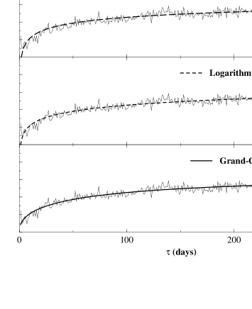
Figure 4: Variogram of the log-volatility, $\langle\log^{2}(\sigma_{t}/\sigma_{t+\tau})\rangle$ as a function of $\tau$, averaged over 17 different stock indices (American, European, Asian). The upper panel shows a fit with a power law of time, the middle panel a fit with the logarithmic (multi-fractal) prediction, whereas the lower panel shows the MG fit Eq. (8), with again both axis rescaled and a constant added to account for the presence of ‘white noise’ trading. Note that the three models lead to nearly indistinguishable fits.

Since the volatility and the volume of activity are strongly correlated also in financial markets [30, 31], our interpretation should carry over to volatility fluctuations as well. This is illustrated in Figure 4 (lower panel), where the variogram of the log-volatility for major stock indices is shown, together with the very same MG fit. Again, the agreement is very good. We have however also shown for comparison the prediction of the multi-fractal model of ref. [6] $V_{a}(\tau)=2\lambda^{2}\log(\tau/\tau_{0})$ (middle panel). We note that the two models, although very different, lead to nearly indistinguishable numerical fits over the time scale considered. In the literature, it is also customary to fit the volatility correlations with power laws. We have therefore also shown in the upper panel the corresponding fit for the variogram $V_{a}(\tau)=c_{0}-c_{1}/\tau^{\nu}$, with $\nu=0.1$. This fit is also consistent with the data (and is numerically very close to a logarithmic function because $\nu$ is small). However, neither the power-law nor the logarithm have clear microscopic motivations. If, as we believe, the simple mechanism that we have advocated is at the origin of the correlations behaviour then the truly universal feature is in the $\sqrt{\tau}$ behaviour of the variogram for small $\tau$, and not in the long time behaviour of the correlation function. In other terms, the exponent $\nu$ might be an effective, non universal exponent masking the true universal $1/2$ exponent that describes the initial increase of the variogram.

In summary, we have proposed a very general interpretation for long-range correlation effects in the activity and volatility of financial markets. This interpretation is based on the fact that the choice between different strategies is subordinated to random-walk like processes. We have numerically demonstrated our scenario in the framework of simplified market models, and showed that, somewhat surprisingly, real market data can actually be quite accurately accounted for by these simple models (see Figs 3 and 4).

Acknowledgments Useful interactions with G. Canat, A. Cavagna, D. Challet, D. Farmer, A. Matacz, E. Moro, J.P. Garrahan, N. Johnson, T. Lux, M. Marsili, M. Potters, P. Seager, D. Sherrington and H. Zytnicki are acknowledged.

References

- [1] Z. Ding, C. W. J. Granger and R. F. Engle, J. Empirical Finance 1, 83 (1993).
- [2] R. Mantegna & H. E. Stanley, An Introduction to Econophysics, Cambridge University Press, 1999.
- [3] J.-P. Bouchaud and M. Potters, Théorie des Risques Financiers, Aléa-Saclay, 1997; Theory of Financial Risks, Cambridge University Press, 2000.
- [4] M. Potters, R. Cont, J.-P. Bouchaud, Europhys. Lett. 41, 239 (1998).
- [5] Y. Liu, P. Cizeau, M. Meyer, C.-K. Peng, H. E. Stanley, Physica A245 437 (1997); P. Cizeau, Y. Liu, M. Meyer, C.-K. Peng, H. E. Stanley, Physica A245 441 (1997).
- [6] A. Arnéodo, J.-F. Muzy, D. Sornette, Eur. Phys. J. B 2, 277 (1998); J.-F. Muzy, J. Delour, E. Bacry, e-print cond-mat/0005400.
- [7] J.-P. Bouchaud, Power in Economics and Finance, some ideas from physics, Quantitative Finance, 1, 105, (2000)
- [8] P. Bak, M. Paczuski, and M. Shubik, Physica A 246, 430 (1997)
- [9] See e.g. W.B. Arthur, Amer. Econ. Assoc. Papers and Proc. 84, 406 (1994); Science, 284, 107 (1999).
- [10] D. Challet, Y.-C. Zhang, Physica A246, 407 (1997)
- [11] J.-P. Bouchaud, R. Cont, European Journal of Physics B 6, 543 (1998); R. Cont, J.P. Bouchaud, Macroeconomics Dynamics, 4, 170 (2000).
- [12] J.D. Farmer, Market Force, Ecology and Evolution, e-print adap-org/9812005, Int. J. Theo. Appl. Fin. 3, 425 (2000).
- [13] D. Sornette, D. Stauffer, H. Takayasu, e-print cond-mat/9909439, and references therein.
- [14] W. Brock, C. Hommes, Econometrica 65, 1059 (1997)
- [15] T. Lux, M. Marchesi, Nature 397, 498 (1999), Int. J. Theo. Appl. Fin. 3, 675 (2000).
- [16] C.H. Hommes, Quantitative Finance 1 149 (2001).
- [17] G. Iori, e-print adap-org/9905005; Int. J. Mod. Phys. C 10, 149 (1999).
- [18] For a review, see J. D. Farmer, Computing in Science and Engineering, November 1999, reprinted in Int. J. Theo. Appl. Fin. 3, 311 (2000).
- [19] J.P. Bouchaud, I. Giardina, M. Mézard, Quantitative Finance, 1, 212 (2001)
- [20] M. Youssefmir, B. Huberman, Journal of Economic Behaviour and Organisation, 32 101 (1997)
- [21] D. Challet, M. Marsili, Y.-C. Zhang, e-print cond-mat/9909265. D. Challet, M. Marsili, R. Zecchina, Int. J. Theo. Appl. Fin. 3, 451 (2000).
- [22] P. Jefferies, M. Hart, P.M. Hui, N. F. Johnson, e-print cond-mat/0008387; Int. J. Theo. Appl. Fin. 3, 443 (2000).
- [23] G. Canat, H. Zytnicki, M. Mézard, Ecole Polytechnique Internal Report (June 2000).
- [24] D. Challet, M. Marsili, Y.-C. Zhang, e-print cond-mat/0101326.
- [25] A. Cavagna, Phys. Rev. E59, R3783 (1999).
- [26] A. Cavagna, J.P. Garrahan, I. Giardina, D. Sherrington, Phys. Rev. Lett. 83, 4429 (1999).
- [27] J.P. Garrahan, E. Moro, D. Sherrington, Phys. Rev. E62, R9 (2000).
- [28] I. Giardina, J.P. Bouchaud, M. Mézard, in preparation.
- [29] C. Godrèche, J.M. Luck, e-print cond-mat/0010428
- [30] G. Bonanno, F. Lillo, R. Mantegna, e-print cond-mat/9912006
- [31] V. Plerou, P. Gopikrishnan, L.A. Amaral, X. Gabaix, H.E. Stanley, e-print cond-mat/9912051.
- [32] Donaldson and Kim, Journ. of International and Comparative Economics 1 86 (1992).