Derivation of a non-objective Oldroyd model from the Boltzmann equation

Abstract

I calculate the hydrodynamic limit of the BGK approximation of the Boltzmann equation for the case of a long stress relaxation time and find that the stress obeys a viscoelastic constitutive equation. The constitutive equation is different from standard constitutive equations used for polymeric liquids in that it is not “objective” because inertial effects are important. I calculate the exact solution for the stresses for simple shear flow and elongational flow.

1 Introduction

It has long been known that not only complex fluids like polymeric liquids show viscoelastic behavior but that even gases show some viscoelasticity [1]. Because these effects are small for gases and difficult to measure in most cases they have only received a more detailed consideration when molecular dynamics simulations showed non-Newtonian behavior in simple shear flow [2] and Zwanzig [3] found an analytical solution for the BGK approximation of the Boltzmann equation that reproduced the shear thinning found in the computer simulations. Examination of the non-Newtonian aspects of flows described by the Boltzmann equation focuses on the case of a simple shear flow [4, 5, 6, 7] and it was analyzed in increasing detail by generalizing the results to hard spheres [5, 6]. Recently the results have been generalized to a perturbative expansion around the simple shear flow by Lee et al. [7].

Giraud and d’Humiéres[8] take a different angle on the non-Newtonian limit of the Boltzmann equation. They have attempted to use the viscoelastic properties hidden in the BGK-Boltzmann equation to define lattice Boltzmann models with viscoelastic properties. So far, however, their results are limited to linear viscoelasticity. We hope that the analytical methods derived in this article can help to direct the research into viscoelastic lattice Boltzmann methods.

In this article we present an intriguingly simple analysis of the moments of the Boltzmann equation in the BGK approximation which allows us to derive a viscoelastic constitutive equation. This constitutive equation has a number of interesting properties. Firstly it is not “objective”, i.e. inertial effects can not be neglected. Secondly the first normal stress difference has a negative sign as compared with a positive sign for polymeric liquids. Unlike the upper-convected Maxwell model used to describe polymeric liquids our constitutive equation shows shear thinning.

In the second part of this article we will show that our constitutive equation reduces to the analytical results derived by Zwanzig[3] for the case of simple shear flow. For this simple situation we then give an intuitive explanation for the difference in viscoelastic behavior for a gas and a polymeric liquid. We also find a new exact solution for the stress for elongational flows.

2 Derivation of viscoelasticity in the BGK Boltzmann equation

The Boltzmann equation was derived for rarefied gases and is a complicated integral equation. However in the hydrodynamic limit the Navier-Stokes equations for fluid flow can be recovered and this is one of the reasons that it is also the basis for a popular method of simulating fluids, the lattice Boltzmann method. All the properties required for the description of a fluid are retained in the somewhat simpler single relaxation time approximation introduced by Bhatnagar et al. [9] (BGK) which is still a complicated non-linear equation. In certain simple situations, however, this equation has an analytical solution [3].

In this section we derive a viscoelastic limit of the BGK approximation[9] of the Boltzmann equation in the limit of large relaxation times. The Boltzmann equation is an evolution equation for probability density $f_{v}({\bf x},t)$ to find a particle at time $t$, at position $\bf x$ with velocity $\bf v$. The evolution equation consists of a free streaming of the particles and a collision term. The effect of the collision term is approximated in the BGK approximation as a simple relaxation of the distribution function towards the equilibrium distribution $f^{0}$. This local equilibrium distribution is the Maxwell-Boltzmann distribution for a given density, velocity and temperature. The evolution equation is

$$\partial_{t}f_{v}+v_{\alpha}\partial_{\alpha}f_{v}=\frac{1}{\tau}(f^{0}_{v}-f_{v})$$ (1)

where the relaxation time $\tau$ is $\tau(\rho,\theta)=\tau_{0}/(\rho T^{b})$. The exponent $b$ can be calculated for molecules with potential $V(r)\sim r^{-l}$ to be $b=1/2-2/l$ [3]. The simplest case is the case of so called Maxwell molecules ($l=4$) for which $b=0$ and there is not $T$-dependence. We define the density $\rho$, the mean velocity $u_{\alpha}$ and the temperature $\theta$ as

$$\int f_{v}dv=\rho,\;\;\;\int f_{v}v_{\alpha}=\rho u_{\alpha},\;\;\;\int f_{v}({\bf v-u})^{2}=D\rho\theta$$ (2)

where $D$ is the number of spatial dimensions. Because of mass, momentum and energy conservation the equilibrium distribution has to have the same moments

$$\int f^{0}_{v}dv=\rho,\;\;\;\int f^{0}_{v}v_{\alpha}=\rho u_{\alpha},\;\;\;\int f^{0}_{v}(v_{\alpha}-u_{\alpha})(v_{\beta}-u_{\beta})=\rho\theta\delta_{\alpha\beta}$$ (3)

and the second moment is isotropic. We can now integrate the Boltzmann equation over the conserved moments $1,{\bf v},{\bf v}^{2}$ corresponding to mass, momentum and energy and get the continuity equation

$$\partial_{t}\rho+\partial_{\alpha}(\rho u_{\alpha})=0$$ (4)

and a momentum conservation equation

$$\rho\partial_{t}u_{\alpha}+\rho u_{\beta}\partial_{\beta}u_{\alpha}=-\partial_{\beta}\Pi_{\alpha\beta}$$ (5)

where

$$\Pi_{\alpha\beta}=\int f_{v}(v_{\alpha}-u_{\alpha})(v_{\beta}-u_{\beta})d{\bf v}$$ (6)

We now need to calculate $\Pi_{\alpha\beta}$ and we split the contribution to $\Pi_{\alpha\beta}$ into an equilibrium and a traceless non-equilibrium part where we use

$$f_{v}=f_{v}^{0}-\tau(\partial_{t}f_{v}+v_{\alpha}\partial_{\alpha}f_{v})$$ (7)

from equation (1).

$$\Pi_{\alpha\beta} = \int f_{v}(v_{\alpha}-u_{\alpha})(v_{\beta}-u_{\beta})d{\bf v}$$ (8)

$$= \int\left[f^{0}_{v}-\tau(\partial_{t}f_{v}+\partial_{\gamma}v_{\gamma}f_{v})\right](v_{\alpha}-u_{\alpha})(v_{\beta}-u_{\beta})$$

$$= \rho\theta\delta_{\alpha\beta}+\sigma_{\alpha\beta}$$

where $\sigma_{\alpha\beta}$ is a traceless stress.

The energy conservation equation is then

$$0 = \int(\partial_{t}f_{v}v_{\alpha}v_{\alpha}+v_{\beta}\partial_{\beta}f_{v}v_{\alpha}v_{\alpha})dv$$ (9)

$$= \partial_{t}(\Pi_{\alpha\alpha}+\rho u_{\alpha}u_{\alpha})$$

$$+\partial_{\beta}(Q_{\beta\alpha\alpha}+\Pi_{\beta\alpha}u_{\alpha}+\Pi_{\alpha\beta}u_{\alpha}+\Pi_{\alpha\alpha}u_{\beta}+\rho u_{\beta}u_{\alpha}u_{\alpha})$$

where $Q$ is related to the third velocity moment of the distribution function

$$Q_{\alpha\beta\gamma} = \int f_{v}(v_{\alpha}-u_{\alpha})(v_{\beta}-u_{\beta})(v_{\gamma}-u_{\gamma})d{\bf v}$$

$$= \int f_{v}v_{\alpha}v_{\beta}v_{\gamma}dv-u_{\alpha}\Pi_{\beta\gamma}-u_{\beta}\Pi_{\alpha\gamma}-u_{\gamma}\Pi_{\alpha\beta}-\rho u_{\alpha}u_{\beta}u_{\gamma}.$$

We can restate the energy conservation equation (9) as

$$\partial_{t}(\rho\theta)+u_{\beta}\partial_{\beta}(\rho\theta) = -\frac{2+D}{D}\rho\theta\partial_{\beta}u_{\beta}-\frac{1}{D}\partial_{\beta}Q_{\beta\alpha\alpha}-\frac{2}{D}\partial_{\beta}u_{\alpha}\sigma_{\alpha\beta}$$ (11)

The equation (8) imposes a constitutive equation for the stress $\sigma_{\alpha\beta}$:

$$\frac{1}{\tau}\sigma_{\alpha\beta} = -\int(\partial_{t}f_{v}+v_{\gamma}\partial_{\gamma}f_{v})(v_{\alpha}-u_{\alpha})(v_{\beta}-u_{\beta})$$ (12)

$$= -\partial_{t}(\rho\theta\delta_{\alpha\beta}+\sigma_{\alpha\beta})-\partial_{\gamma}u_{\beta}(\rho\theta\delta_{\alpha\gamma}+\sigma_{\alpha\gamma})$$

$$-\partial_{\gamma}u_{\alpha}(\rho\theta\delta_{\gamma\beta}+\sigma_{\gamma\beta})-\partial_{\gamma}u_{\gamma}(\rho\theta\delta_{\alpha\beta}+\sigma_{\alpha\beta})$$

$$-u_{\gamma}\partial_{\gamma}(\rho\theta\delta_{\alpha\beta}+\sigma_{\alpha\beta})-\partial_{\gamma}Q_{\alpha\beta\gamma}$$

Using the equation for the energy conservation we get for the $\theta$ terms

$$\partial_{t}(\rho\theta)\delta_{\alpha\beta}+u_{\gamma}\partial_{\gamma}(\rho\theta)\delta_{\alpha\beta}+\rho\theta(\partial_{\beta}u_{\alpha}+\partial_{\alpha}u_{\beta}+\partial_{\gamma}u_{\gamma}\delta_{\alpha\beta})$$ (13)

$$= \rho\theta(\partial_{\beta}u_{\alpha}+\partial_{\alpha}u_{\beta}-\frac{2}{D}\partial_{\gamma}u_{\gamma}\delta_{\alpha\beta})+\frac{2}{D}\partial_{\gamma}u_{\delta}\sigma_{\gamma\delta}-\frac{1}{D}\partial_{\gamma}Q_{\gamma\delta\delta}.$$

Introducing a convected time derivative as

$$\sigma_{\alpha\beta<1>}=D_{t}\sigma_{\alpha\beta}+(\partial_{\gamma}u_{\alpha}\sigma_{\gamma\beta}+\sigma_{\alpha\gamma}\partial_{\gamma}u_{\beta}),$$ (14)

where the total derivative is $D_{t}=\partial_{t}+v_{\alpha}\partial_{\alpha}$, we can now write the constitutive equation as

$$\sigma_{\alpha\beta}+\tau\sigma_{\alpha\beta<1>}-\tau\frac{2}{D}(\sigma_{\gamma\delta}\partial_{\delta}u_{\gamma})\delta_{\alpha\beta}+\tau\partial_{\gamma}u_{\gamma}\sigma_{\alpha\beta}$$ (15)

$$= -\tau\rho\theta(\partial_{\alpha}u_{\beta}+\partial_{\beta}u_{\alpha}-\frac{2}{D}\partial_{\gamma}u_{\gamma}\delta_{\alpha\beta})-\tau\partial_{\gamma}Q_{\alpha\beta\gamma}+\tau\frac{1}{D}\partial_{\gamma}Q_{\gamma\delta\delta}\delta_{\alpha\beta}$$

This expression is similar to the stress relaxation equation proposed by Maxwell[1] and we get his result if we replace the convected derivative with a partial time derivative. Eqn. (15) was first derived in its complete form from an expansion of the full Boltzmann equation in Hermite polynomials by Grad[10].

The usual expansion of the Boltzmann equation in the hydrodynamic limit is done under the assumption $\tau=O(1)$ and $\partial=O(\epsilon)$. Then we get for the leading order of the stress (of order $\epsilon$)

$$\sigma=-\tau\rho\theta\left(\nabla u+(\nabla u)^{\dagger}-\frac{2}{D}tr(\nabla u)\delta\right)$$ (16)

For larger relaxation times, however, we obtain a viscoelastic result. We keep the assumption that derivatives are small to order epsilon $\partial=O(\epsilon)$ but keep terms up to order $O(\epsilon^{2})$. We now get to leading order $O(\epsilon^{2})$ the full equation (15) but the terms containing $Q$ still need to be expressed in terms of macroscopic quantities. The contribution of the equilibrium distribution to $Q$ vanishes so it is useful to express $Q$ in terms of the first order non-equilibrium contributions. If we iteratively substitute eqn. (7) twice into eqn.(2) we can write

$$Q_{\alpha\beta\gamma} = -\tau\left(\int\partial_{t}f^{0}_{v}(v_{\alpha}-u_{\alpha})(v_{\beta}-u_{\beta})(v_{\gamma}-u_{\gamma})\right.$$ (17)

$$\left.+\int\partial_{\delta}f^{0}_{i}v_{\delta}(v_{\alpha}-u_{\alpha})(v_{\beta}-u_{\beta})(v_{\gamma}-u_{\gamma})\right)+O(\partial^{2})$$

$$= \tau\left\{\int f^{0}_{i}\partial_{t}\left[(v_{\alpha}-u_{\alpha})(v_{\beta}-u_{\beta})(v_{\gamma}-u_{\gamma})\right]\right.$$

$$\left.+\int f^{0}_{i}v_{\delta}\partial_{\delta}\left[(v_{\alpha}-u_{\alpha})(v_{\beta}-u_{\beta})(v_{\gamma}-u_{\gamma})\right]\right.$$

$$\left.-\partial_{\delta}\int f^{0}_{v}(v_{\alpha}-u_{\alpha})(v_{\beta}-u_{\beta})(v_{\gamma}-u_{\gamma})(v_{\delta}-u_{\delta})\right\}+O(\partial^{2})$$

$$= -\tau\left\{(\delta_{\alpha\beta}\delta_{\gamma\delta}+\delta_{\alpha\gamma}\delta_{\beta\delta}+\delta_{\alpha\delta}\delta_{\beta\gamma})\partial_{\delta}(\rho\theta^{2})\right.$$

$$\left.+(\partial_{t}u_{\alpha}+u_{\delta}\partial_{\delta}u_{\alpha})\rho\theta\delta_{\beta\gamma}+(\partial_{t}u_{\beta}+u_{\delta}\partial_{\delta}u_{\beta})\rho\theta\delta_{\alpha\gamma}\right.$$

$$\left.+(\partial_{t}u_{\gamma}+u_{\delta}\partial_{\delta}u_{\gamma})\rho\theta\delta_{\alpha\beta}\right\}+O(\partial^{2})$$

$$= -\tau\left\{(\delta_{\alpha\beta}\delta_{\gamma\delta}+\delta_{\alpha\gamma}\delta_{\beta\delta}+\delta_{\alpha\delta}\delta_{\beta\gamma})\partial_{\delta}(\rho\theta^{2})\right.$$

$$\left.-(\delta_{\alpha\beta}\delta_{\gamma\delta}+\delta_{\alpha\gamma}\delta_{\beta\delta}+\delta_{\alpha\delta}\delta_{\beta\gamma})\theta\partial_{\delta}(\rho\theta)\right\}+O(\partial^{2})$$

$$= -\tau\rho\theta(\delta_{\alpha\beta}\delta_{\gamma\delta}+\delta_{\alpha\gamma}\delta_{\beta\delta}+\delta_{\alpha\delta}\delta_{\beta\gamma})\partial_{\delta}\theta+O(\partial^{2})$$

which is the only approximation we have to make. We then get for the $Q$ terms in eqn. (16)

$$\partial_{\gamma}Q_{\alpha\beta\gamma}-\frac{1}{D}\partial_{\gamma}Q_{\gamma\delta\delta}\delta_{\alpha\beta}$$ (18)

$$= -\partial_{\alpha}(\tau\rho\theta\partial_{\beta}\theta)-\partial_{\beta}(\tau\rho\theta\partial_{\alpha}\theta)+\frac{2}{D}\partial_{\gamma}(\tau\rho\theta\partial_{\gamma}\theta)\delta_{\alpha\beta}+O(\epsilon^{2})$$

$$= -\tau\rho\theta\left(2\partial_{\alpha}\partial_{\beta}-\frac{2}{D}\partial_{\gamma}\partial_{\gamma}\delta_{\alpha\beta}\right)+O(\epsilon^{2})$$

where we have used $\tau(\rho\theta)=\tau_{0}/(\rho\theta)$ in the last line. So the viscoelastic constitutive equation is

$$\sigma_{\alpha\beta}+\tau\sigma_{\alpha\beta<1>} = \tau\rho\theta(\partial_{\alpha}u_{\beta}+\partial_{\beta}u_{\alpha}-\frac{2}{D}\partial_{\gamma}u_{\gamma}\delta_{\alpha\beta})$$ (19)

$$-\tau\rho\theta\left(2\partial_{\alpha}\partial_{\beta}-\frac{2}{D}\partial_{\gamma}\partial_{\gamma}\right)\theta+O(\epsilon^{3})$$

where the last term in $\theta$ represents stresses induced by second derivatives of the temperature. Note that this constitutive equation is exact if second order derivatives vanish.

3 Comparison to usual “objective” constitutive equations

In the theory of viscoelastic constitutive equations usually the assumption is made that the constitutive equation should be invariant under an arbitrary transformation that preserves distances and time intervals [11]. That also requires form-invariance of the constitutive equation under some non-inertial transformations such as rotations and accelerated systems. The underlying idea is that the stresses in a polymeric fluid only the stretching of the system is relevant and all inertial contributions can be neglected. In particular a convected time derivative that obeys this symmetry is said to be an “objective time derivative”.

There are two such derivatives; the upper convected derivative

$$\sigma_{\alpha\beta(1)}=D_{t}\sigma_{\alpha\beta}-(\partial_{\gamma}u_{\alpha}\sigma_{\gamma\beta}+\sigma_{\alpha\gamma}\partial_{\gamma}u_{\beta})$$ (20)

and the lower convected derivative

$$\sigma_{\alpha\beta}^{(1)}=D_{t}\sigma_{\alpha\beta}+(\partial_{\alpha}u_{\gamma}\sigma_{\gamma\beta}+\sigma_{\alpha\gamma}\partial_{\beta}u_{\gamma}).$$ (21)

Any linear combination of these two is also objective, and in the past the Jaumann derivative given by $(\sigma_{\alpha\beta(1)}+\sigma_{\alpha\beta}^{(1)})/2$ has been popular. Today, however, constitutive equations for viscoelastic fluids are constructed with a broad preference for the upper convected derivative because these agree best with the new experimental results [11].

Many frequently used constitutive models are contained in the rather general Oldroyd 8-constant model [11, 7.3-2]. If we only keep constants that can be related to our constitutive equation we get

$$\sigma_{\alpha\beta}+\lambda_{1}\sigma_{\alpha\beta(1)}+\frac{1}{2}\lambda_{6}\partial_{\gamma}u_{\delta}\sigma_{\delta\gamma}\delta_{\alpha\beta}=-\eta_{0}(\partial_{\alpha}u_{\beta}+\partial_{\beta}u_{\alpha})$$ (22)

as a special case of the Oldroyd 8-constant model. This is identical to our constitutive model of eqn.(19) up to the sign change between $\sigma_{\alpha\beta(1)}$ and $\sigma_{\alpha\beta<1>}$ if we consider that the Oldroyd model is only derived for incompressible fluids ($\partial_{\gamma}u_{\gamma}=0$) and does not consider elastic effects of temperature gradients ($\partial\theta=0$). It is interesting to note that the most frequently used special cases of the Oldroyd 8-constant model all assume that $\lambda_{6}=0$. (The equation above with $\lambda_{6}=0$ is known as the upper convected Maxwell model).

The difference between the Oldroyd model and our constitutive equation lies purely in the nature of the convected derivatives $\sigma_{(1)}$ of eqn. (20) and $\sigma_{<1>}$ of eqn. (14) which is mathematically a difference in the sign of the $\partial u\sigma$ terms. In particular this means that the new convected derivative is not “objective”. It is not too surprising, however, that inertial effects are important for a gas and therefore there is no reason to require an objective derivative for the viscoelastic constitutive equation of a gas. We will be discussing the effect of this subtle difference for two special cases, the simple shear flow and the elongational flow and give also an intuitive explanation for the differences in the next section.

3.1 Simple shear flow

The most studied situation is probably the simple shear flow with velocity profile

$${\bf u}=\left(\begin{array}[]{c}\dot{\gamma}y\\ 0\\ 0\end{array}\right)$$ (23)

where $\dot{\gamma}$ is the shear rate. The stress is then given by

$$\sigma=\left(\begin{array}[]{ccc}\sigma_{xx}&\sigma_{xy}&0\\ \sigma_{xy}&\sigma_{yy}&0\\ 0&0&\sigma_{zz}\end{array}\right)$$ (24)

and we obtain the differential equations for the stress terms

$$\sigma_{xx}+\tau\partial_{t}\sigma_{xx} = \tau\left(\frac{2}{3}-2\right)\dot{\gamma}\sigma_{xy}$$ (25)

$$\sigma_{yy}+\tau\partial_{t}\sigma_{yy} = \tau\frac{2}{3}\dot{\gamma}\sigma_{xy}$$ (26)

$$\sigma_{xy}+\tau\partial_{t}\sigma_{xy}+\tau\dot{\gamma}\sigma_{yy} = -\tau\rho\theta\dot{\gamma}$$ (27)

To close this system of equations we also need the heat equation (11) which reads for a spatially constant temperature and a divergence free velocity field

$$\partial_{t}(\rho\theta)=-\frac{2}{D}\partial_{\alpha}u_{\beta}\sigma_{\beta\alpha}$$ (28)

We now make the Ansatz

$$\sigma_{\alpha\beta}(\theta)=\rho\theta\hat{\sigma}_{\alpha\beta}$$ (29)

so that we get from (28) for the time dependence of the temperature

$$\theta(t)=\theta_{0}\exp\left(-\frac{2}{D}\partial_{\alpha}u_{\beta}\hat{\sigma}_{\beta\alpha}t\right)$$ (30)

which reads for the velocity field of eqn. (23)

$$\theta(t)=\theta_{0}\exp\left(-\frac{2}{3}\dot{\gamma}\hat{\sigma}_{xy}t\right).$$ (31)

So the differential equations for $\sigma$ become algebraic equations

$$\sigma_{xx}+\tau\left(-\frac{2}{3}\dot{\gamma}\hat{\sigma}_{xy}\right)\sigma_{xx} = \tau\left(\frac{2}{3}-2\right)\dot{\gamma}\sigma_{xy}$$ (32)

$$\sigma_{yy}+\tau\left(-\frac{2}{3}\dot{\gamma}\hat{\sigma}_{xy}\right)\sigma_{yy} = \tau\frac{2}{3}\dot{\gamma}\sigma_{xy}$$ (33)

$$\sigma_{xy}+\tau\left(-\frac{2}{3}\dot{\gamma}\hat{\sigma}_{xy}\right)\sigma_{xy}+\tau\dot{\gamma}\sigma_{yy} = -\tau\rho\theta\dot{\gamma}$$ (34)

Thus we arrive at a cubic equation for $\sigma_{xy}$

$$\left(\frac{2}{3}\,\frac{\tau\dot{\gamma}}{\rho\theta}\sigma_{xy}-1\right)^{2}\sigma_{xy}=-\tau\rho\theta\dot{\gamma}$$ (35)

The solution can be written in analytic terms for $\tau=\tau_{0}/\rho$ as

$$\theta(t) = \theta_{0}\exp(t\lambda)$$ (36)

$$\sigma_{xx} = \rho\theta(t)\left(\frac{1}{1+\tau\lambda}+\frac{2\tau^{2}\dot{\gamma}^{2}}{(1+\tau\lambda)^{3}}\right)$$ (37)

$$\sigma_{yy} = \rho\theta(t)\frac{1}{1+\tau\lambda}$$ (38)

$$\sigma_{zz} = \rho\theta(t)\frac{1}{1+\tau\lambda}$$ (39)

$$\sigma_{xy} = -\frac{3}{2}\rho\theta(t)\frac{\lambda}{\dot{\gamma}}$$ (40)

with

$$\lambda=\frac{4}{3\tau}\sinh^{2}\left(\frac{1}{6}\cosh^{-1}(1+9\tau^{2}\dot{\gamma}^{2})\right)$$ (41)

which is also the exact solution for the BGK approximation of the Boltzmann equation first described by Zwanzig [3] where he derived $f_{v}(t)$ from eqn. (1) for a simple shear flow. He then used this solution in the equivalent of eqn. (8) to determine the stress. We have neglected transient terms which are decaying exponentially. We recover the exact result because our approximation of eqn.(17) become exact for spatially constant temperature.

There are three invariants of the stress tensor which are defined as $\sigma_{xy}=-\eta\dot{\gamma}$ related to the viscosity $\eta$, $\sigma_{xx}-\sigma_{yy}=-\Psi_{1}\dot{\gamma}^{2}$ related to the first normal stress coefficient $\Psi_{1}$, and $\sigma_{yy}-\sigma_{zz}=-\Psi_{2}\dot{\gamma}^{2}$ related to the second normal stress coefficient $\Psi_{2}$. For our constitutive equation we get

$$\eta=\frac{\tau\rho\theta}{(1+\tau\lambda)^{2}}\;\;\;\Psi_{1}=-\frac{2\tau\eta}{1+\tau\lambda}\;\;\;\Psi_{2}=0$$ (42)

In this simple situation we get a result that is equivalent to that of an upper convected Maxwell model but with the opposite sign for the first normal stress difference. Viscoelastic polymeric systems for which the upper convected Maxwell model was devised seem to always have a positive first normal stress coefficient $\Psi_{1}$. In the next section we will give some intuitive understanding for this fundamental difference in the viscoelasticity.

$\frac{\eta(\dot{\gamma})}{\eta_{0}}$

$\dot{\gamma}$

$\frac{-\Psi_{1}(\dot{\gamma})}{2\tau\rho\theta}$

$\dot{\gamma}$

Figure 1: The exact solution for the shear-rate dependent viscosity $\eta(\dot{\gamma})$ and first normal stress difference $\Psi_{1}(\dot{\gamma})$ against the shear rate $\dot{\gamma}$ (full line) and the isothermal solution (broken line). See text for details.

Although for a simple shear flow no stationary solution exists due to viscous heating a stationary state can be achieved with the help of a thermostat. The simplest way of implementing a thermostat is simply to assume that the partial time derivatives and the spatial derivatives of the temperature in eqns (25)-(28) vanishes [8, 11]. This is equivalent to a situation where a thermostat insures a constant temperature, but does not otherwise influence the dynamics. This thermostat will change the energy equation but not the constitutive equation. In this case we get

$$\eta=\frac{\tau\rho\theta}{1+\frac{2}{3}\tau^{2}\dot{\gamma}^{2}}\;\;\;\Psi_{1}=-2\tau\eta\;\;\;\Psi_{2}=0$$ (43)

and we see that the shear-thinning persists although it now has a different form. The first normal stress difference now only depends on the shear rate through the viscosity. The viscosity and the first normal stress difference for the isothermal and the heating case are compared in Figure 1. Other thermostats lead to different results. Lee and Dufty [7] considered a thermostat that is frequently used for Molecular Dynamics simulations. This thermostat rescales the local velocities relative to the average velocities such that the temperature remains constant. In this case the constitutive equation is also changed but in a way that recovers the same solution 42 as in the case with heating, except that the temperature remains constant.

3.2 Extensional flow

We will now consider a second family of flow-fields for which, to my knowledge, the BGK equations had not previously been solved. We will, again, assume a spatially constant temperature so that the results will be exact. And extensional flow is a shear-free flow defined by the velocity profile

$${\bf u}=\dot{\epsilon}\left(\begin{array}[]{c}-(1+b)x/2\\ -(1-b)y/2\\ z\end{array}\right)$$ (44)

where $0\leq b\leq 1$ and $\dot{\epsilon}$ is the elongation rate. Several special shear-free flows are obtained for particular choices of the parameter $b$:

Elongational flow: $(b=0,\dot{\epsilon}>0)$

Biaxial stretching flow: $(b=0,\dot{\epsilon}<0)$

Planar elongational flow: $(b=1)$

For the time-dependence of the temperature we get from eqn. (30) for the extensional flow

$$\theta(t)=\theta_{0}\exp\left(-\frac{\dot{\epsilon}}{3}(-(1+b)\hat{\sigma}_{xx}-(1-b)\hat{\sigma}_{yy}+2\sigma_{zz})t\right).$$ (45)

The flow is a linear flow and if we assume a constant initial temperature the solutions of the constitutive equation are again exact. For the constitutive equation for the stress (19), using that $\sigma_{xx}+\sigma_{yy}+\sigma_{zz}=0$, we get

$$(\frac{1}{\tau\dot{\epsilon}}-(1+b))\hat{\sigma}_{xx}+\left((1+\frac{b}{3})\hat{\sigma}_{xx}+(1-\frac{b}{3})\hat{\sigma}_{yy}\right)\left(1+\hat{\sigma}_{xx}\right) = 1+b$$ (46)

$$(\frac{1}{\tau\dot{\epsilon}}-(1-b))\hat{\sigma}_{yy}+\left((1+\frac{b}{3})\hat{\sigma}_{xx}+(1-\frac{b}{3})\hat{\sigma}_{yy}\right)\left(1+\hat{\sigma}_{yy}\right) = 1-b$$ (47)

These equations have analytic solutions one of which is physical. These results, however, are too lengthy to be presented here. For the simpler case of $b=0$ the $x$ and $y$ directions are symmetric and so we can impose $\sigma_{xx}=\sigma_{yy}$ and the equations can be simplified to

$$(\frac{1}{\tau\dot{\epsilon}}-1)\hat{\sigma}_{xx}+2\hat{\sigma}_{xx}\left(1+\hat{\sigma}_{xx}\right)=1$$ (48)

This equation has two solutions but one of these solutions is unphysical as the stress is larger that $\rho\theta$ which would require a negative probability density $f_{v}$ in (8). The physical solution is

$$\sigma_{xx}=-\frac{\rho\theta}{4}\frac{1+\tau\dot{\epsilon}-\sqrt{1+2\tau\dot{\epsilon}+9\tau^{2}\dot{\epsilon}^{2}}}{\tau\dot{\epsilon}}$$ (49)

and $-\sigma_{zz}/2=\sigma_{yy}=\sigma_{xx}$.

$\frac{\bar{\eta}_{1}}{\rho\theta},\frac{\bar{\eta}_{2}}{\rho\theta}$

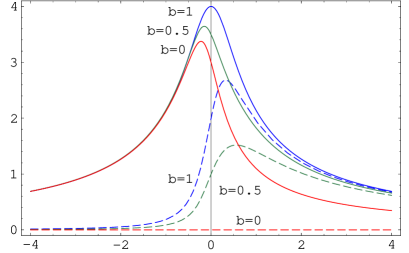
$\tau\dot{\epsilon}$

Figure 2: The exact solution for the extension-rate dependent elongational viscosities $\bar{\eta}_{1}$(full lines) and $\bar{\eta}_{2}$(dashed lines) for different parameters b (see text for details).

It is customary to define two viscosity functions to describe the rheological behaviour of a fluid in extensional flow [11] as

$$\sigma_{xx}-\sigma_{zz} = \bar{\eta}_{1}(\dot{\epsilon},b)\dot{\epsilon}$$ (50)

$$\sigma_{xx}-\sigma_{yy} = \bar{\eta}_{2}(\dot{\epsilon},b)\dot{\epsilon}$$ (51)

and we show the values for different $b$ in Figure 2. For the elongational flow and the biaxial stretching flow ($b=0$) defined above the $x$ and $y$-directions are equivalent and therefore $\bar{\eta}_{2}=0$. For the elongational flow ($b=0,\dot{\epsilon}>0$) we find only shear thinning (in polymeric flows a shear-thickening is observed) but for the biaxial stretching flow gases show a shear thickening.

For the planar elongational flow $b=1$ the $x$ and $z$ directions become symmetric if you invert the extension rate ($\sigma_{xx}(\dot{\epsilon},b=1)=\sigma_{zz}(-\bar{\epsilon},b=1)$) so that the viscosity $\bar{\eta}_{1}$ becomes symmetric, but the viscosity $\bar{\eta}_{2}$ becomes asymmetric. Even though the planar elongational flow is a two-dimensional flow the stress will be different for a true two-dimensional system and this three dimensional case.

If we consider a system with a simple-minded thermostat again that simply assumes a constant temperature we get unphysical divergences for the stress

$$\sigma_{xx} = \tau\rho\theta\dot{\epsilon}\frac{3(1+b)+\tau\dot{\epsilon}(-3+6b+b^{2})}{-3+(3+b^{2})\tau^{2}\dot{\epsilon}^{2}}$$ (52)

$$\sigma_{yy} = \tau\rho\theta\dot{\epsilon}\frac{3(1-b)+\tau\dot{\epsilon}(-3-6b+b^{2})}{-3+(3+b^{2})\tau^{2}\dot{\epsilon}^{2}}$$ (53)

$$\sigma_{zz} = 2\tau\rho\theta\dot{\epsilon}\frac{-3+\tau\dot{\epsilon}(3-b^{2})}{-3+(3+b^{2})\tau^{2}\dot{\epsilon}^{2}}$$ (54)

but the quadratic behaviour for small $\dot{\epsilon}$ still agrees with the non-isothermal case. These divergences indicate that the simple-minded thermostat is unphysical.

It is easy to see why this unphysical behavour can occur. Because the thermostat will regulate the temperature without influencing the stress we can have a second moment

$$\Pi_{xx}=\int f_{v}(v_{x}-u_{x})^{2}$$ (55)

that becomes negative which in terms reqires negative contributions to the probability distribution. This is what makes the thermostat unphysical.

(a)

(b)

Figure 3: Illustration of the origin of a non-diagonal pressure $\Pi$ and the corresponding stress tensor $\sigma$ in the case of a gas. (a) Origin of pressure tensor (b) the traceless stress tensor (vectors pointing inwards represent a negative stress). Note that the orientation of the stress tensor we have $\theta_{g}\geq 45\circ$.

Figure 4: Sketch of the origin and orientation of the non-diagonal stress tensor for a polymeric liquid in a simple shear flow. The stress looks qualitatively similar to the gas case of Figure 3 but note that here $\theta_{p}\leq 45^{\circ}$. Also there is no requirement for the polymeric stress to be traceless.

4 Intuition for the viscoelastic effects in a gas

In Figures 3 and 4 we sketched the origins of the non-isotropic stress for both the case of a gas and the case of a polymeric liquid in a simple shear flow. In a gas the mean velocity of the particles is given by the flow profile of equation (23). Particles that are convected in the direction of $-y$ carry more x-momentum with them than the average at this position and particles that are convected in the direction of $+y$ carry less x-momentum with them that the average that the new position. Therefore the momentum distribution will be non-isotropic as indicated in Figure 3(a). If we subtract the isotropic part of the momentum distribution we get the stress tensor $\sigma$ of equation (8) shown in Figure 3(b). Note that the angle $\theta_{g}$ defined in this Figure is always smaller that $45^{\circ}$. Therefore the non-equilibrium stress tends to reduce the force on the walls which is equivalent to a negative first normal stress coefficient.

In simple shear flow the viscosity is a measure for the transport of x-momentum in the y-direction. Because there are now fewer particles streaming in the y-directions this also means that the viscosity is reduced. This is the intuitive reason for the shear thinning in a gas.

In the case of a polymeric liquid the origin of the non-isotropic stress lies in the stretching of the macromolecules as sketched in Figure 4. In equilibrium without flow the macromolecules would curl up into a spherical shape but the flow tends to deform the shape to a more ellipsoidal from. The result is a restoring force that would restore the molecule to a spherical shape. The first deformation of the molecule occurs at $\theta_{p}=45^{\circ}$ and increases from there on. The effect is that the stress distribution sketched in Figure 4 increases the pressure in the y-direction relative to the pressure in the x-direction which is equivalent to a positive first normal stress coefficient.

The deformation of the coils also means that there is less transport of x-momentum in the y-direction which is the reason for shear-thinning in the polymeric liquid.

5 Conclusions

We have derived a viscoelastic constitutive equation for a gas described by the BGK approximation of the Boltzmann equation and shown that this constitutive equation differs substantially from those that describe the viscoelastic properties of polymeric materials. For simple shear flow the exact results for the BGK approximation of the Boltzmann equation are recovered. We explained the different sign of the first normal stress difference in gases and polymeric liquids be examining the qualitative different origins of the non-Newtonian stress.