Probing spin-charge separation in tunnel-coupled parallel quantum wires

Abstract

Interactions in one-dimensional (1D) electron systems are expected to cause a dynamical separation of electronic spin and charge degrees of freedom. A promising system for experimental observation of this non-Fermi-liquid effect consists of two quantum wires coupled via tunneling through an extended uniform barrier. Here we consider the minimal model of an interacting 1D electron system exhibiting spin-charge separation and calculate the differential tunneling conductance as well as the density-density response function. Both quantities exhibit distinct strong features arising from spin-charge separation. Our analysis of these features within the minimal model neglects interactions between electrons of opposite chirality and applies therefore directly to chiral 1D electron systems realized, e.g., at the edge of integer quantum-Hall systems. Physical insight gained from our results is useful for interpreting current experiment in quantum wires as our main conclusions still apply with nonchiral interactions present. In particular, we discuss the effect of charging due to applied voltages, and the possibility to observe spin-charge separation in a time-resolved experiment.

I Introduction

One-dimensional (1D) electron systems are one of the theoretically best-studied examples where interactions lead to strong correlations such that low-energy excitations cannot be described using Landau’s Fermi-liquid concept.[1] As soon as electron-electron interactions are switched on, electron-like quasiparticles cease to exist at low energies, and the elementary excitations are phonon-like charge and spin-density fluctuations, and topological zero modes. Physical quantities of such a Luttinger liquid[2] are determined by the velocities,[3] $v_{\rho}$ and $v_{\sigma}$, of the charge and spin-density phonons, as well as additional velocity parameters characterizing the energy of topological modes. The most striking non-Fermi-liquid feature is exhibited by the single-electron spectral function ${\mathcal{A}}(k,\varepsilon)$ which is basically a measure of the integrity of an electron as an elementary excitation in a many-body system.[4] In the absence of electron-electron interactions, the spectral function is given by ${\mathcal{A}}^{(0)}(k,\varepsilon)=2\pi\delta(\varepsilon-\varepsilon_{k})$ where $\varepsilon_{k}$ is the electronic band dispersion. For an interacting system, the spectral function is generally broadened. However, in a Fermi liquid, ${\mathcal{A}}(k,\varepsilon)$ still exhibits a distinct single-electron-like peak, making it possible to represent the system of interacting electrons as a system of non-interacting quasiparticles that carry the same quantum numbers as free electrons. Such a quasiparticle peak is absent in the spectral function of a Luttinger liquid. Instead, a characteristic double-peak structure appears.[5, 6] The existence of the two peaks whose energy dispersions follow those of the elementary charge and spin-density excitations can be interpreted as the dynamical break-up of the electron into two independent entities representing its spin and charge degrees of freedom.[7]

Experimental verification of spin-charge separation essentially requires a direct measurement of ${\mathcal{A}}(k,\varepsilon)$, e.g., by photoemission[8] or tunneling[9, 10] spectroscopy. Recent progress in fabrication techniques has made it possible to create a system of two parallel quantum wires that are separated by a long and clean tunnel barrier.[11] Uniformity of tunneling between the two quantum wires, labeled U(pper) and L(ower), respectively, implies that canonical momentum is approximately conserved in a single tunneling event. The possibility to tune canonical versus kinetic momentum by an external magnetic field makes it possible to perform momentum-resolved tunneling studies.[12] For example, in a 1D Fermi liquid, resonances appear in the magnetic-field dependence of the linear tunneling conductance whenever Fermi points from different wires overlap,[13, 14] i.e., when for any $\alpha,\alpha^{\prime}=\pm$ the parameter

$$\kappa_{\alpha\alpha^{\prime}}=\frac{\pi}{2}\left(\alpha^{\prime}\,n_{\text{U}}-\alpha\,n_{\text{L}}\right)+\frac{e}{\hbar}B\,d$$ (1)

vanishes. [Here, $n_{\text{U(L)}}$ denotes the 1D electron density in the U (L) wire when no voltage is applied, $B$ is the magnetic field applied perpendicular to the plane defined by the two wires, and $d$ their separation.] Close to these resonance condition of Eq. (1), the differential tunneling conductance (DTC) as a function of voltage and magnetic field can be expected to show features arising from spin-charge separation. This motivates the first part of our study, detailed in Sec. II, where we calculate the DTC to lowest order in perturbation theory close to the resonance point corresponding to $\alpha=\alpha^{\prime}=+$ for a model 1D electron system where interactions between electrons with opposite chirality are neglected. It turns out that charging[15] in response to the applied voltage significantly alters tunneling characteristics. We expect this finding to hold also in the realistic case of non-chiral quantum wires.[16] Detailed expressions are given for the location of four characteristic maxima in the DTC that are a manifestation of spin-charge separation.[17]

A perturbative treatment of tunneling is valid only for calculating physical properties above an, in general, interaction-dependent[18] energy scale. In the absence of interactions, this scale is given by the tunneling strength $|t|$, and the regime where perturbation theory fails is characterized by spatial and temporal oscillations in electronic correlation functions.[13] These oscillations result from coherent electron motion between the two systems.[19] In Sec. III, we provide a theoretical framework to treat the nonperturbative regime with interactions present using bosonization[20, 21] and refermionization[22, 23] techniques. In analogy with previous results,[21] a characteristic length scale $L_{\text{int}}=\pi\hbar|v_{\rho-}-v_{\sigma}|/|2t|$ emerges from our calculation, measuring the relative strengths of tunneling and interactions. On length scales shorter than $L_{\text{int}}$, tunneling is irrelevant, i.e., it does not affect the electronic structure of the two wires.[21] In the opposite limit of large length scales, however, we identify spatial oscillations in the density response with a wave length $L_{t}=\pi\hbar\sqrt{v_{\rho-}v_{\sigma}}/|t|$ that is renormalized from its value $\pi\hbar v_{\text{F}}/|t|$ in the noninteracting limit. In addition, we show a peculiar mode splitting to occur in the density response that is similar to the one found previously[20, 21] for the single-electron Greens function. Besides characteristic charge-mode velocities $v_{\rho\pm}$, an additional velocity $\bar{v}=2v_{\rho-}v_{\sigma}/(v_{\rho-}+v_{\sigma})$ appears in the density response that should be observable, in principle, in a time-resolved experiment. Its existence is a manifestation of spin-charge separation in the tunnel-coupled double-wire system. The naive expectation that the density response is sensitive just to the charge mode is satisfied only in the previously mentioned limit where interactions dominate tunneling.

In our study of spin-charge separation in tunnel-coupled quantum wires, we consider a particular model for an interacting 1D electron system. To be specific, the wires are assumed to be parallel to the $x$ direction, located at $y=0$ and $z=z_{\text{U,L}}$, respectively. The Hamiltonian is given by

$$H = H_{0}+H_{\text{tun}}+H_{\text{int}}\quad,$$ (3)

$$H_{0} = \sum_{k\sigma\atop\alpha\beta}[\alpha\hbar v_{\text{F}\beta}\left(k-\alpha k_{\text{F}\beta}\right)+\nu_{\beta}\,eV_{\beta}]\,c_{k\sigma\alpha\beta}^{\dagger}c_{k\sigma\alpha\beta}\,,$$ (4)

$$H_{\text{tun}} = t\sum_{k\sigma\alpha}\left\{c_{k\sigma\alpha\text{U}}^{\dagger}c_{k\sigma\alpha\text{L}}+c_{k\sigma\alpha\text{L}}^{\dagger}c_{k\sigma\alpha\text{U}}\right\}\,,$$ (5)

$$H_{\text{int}} = \frac{1}{2L}\sum_{\alpha q\atop\beta\beta^{\prime}}U_{\beta\beta^{\prime}}\,\bigg{(}\sum_{\sigma}\varrho_{q\sigma\alpha\beta}\bigg{)}\,\bigg{(}\sum_{\sigma^{\prime}}\varrho_{-q\sigma^{\prime}\alpha\beta^{\prime}}\bigg{)}\,.$$ (6)

Indices $\beta,\beta^{\prime}=\text{U,L}$ distinguish between the upper and lower wire, and $\alpha=\pm$ between right-movers and left-movers. Spin quantum numbers are denoted by $\sigma,\sigma^{\prime}$. Each wire’s Fermi wave vector $k_{\text{F}\beta}=\frac{\pi}{2}n_{\beta}+\frac{eB}{\hbar}\,z_{\beta}$ contains the effect of a magnetic field[24] $\vec{B}=B\,\hat{y}$. A voltage $V_{\text{U(L)}}$ is applied to the U (L) wire, and (in general, voltage-dependent) parameters $\nu_{\beta}$ measure the resulting shift of electron bands.[25] The wires are coupled by a tunneling matrix element $t$ chosen to be real. Fourier transforms of the density of spin-$\sigma$ electrons from the $\alpha$ branch in the $\beta$ wire are denoted by $\varrho_{q\sigma\alpha\beta}$. Interactions included in $H_{\text{int}}$ are chiral, i.e., only electrons from the same branch (right-moving or left-moving) within each wire and between the two wires interact. This model applies directly to interacting edge channels in quantum-Hall bilayers[26] when each layer is at filling factor 2 and Zeeman splitting is negligible. Interactions between left-moving and right-moving electrons which are present in real quantum wires are not accounted for in our model. It turns out, however, that strong features arising from spin-charge separation are accurately described already by the chiral model.[6, 21, 9] For example, the redistribution of spectral weight due to non-chiral interactions leads only to small additional structure in the DTC.[10, 17] Possibilities to go beyond the chiral model are discussed in Sec. III.

II Perturbative treatment

Results presented in this section are obtained within lowest-order perturbation theory in the tunneling Hamiltonian displayed in Eq. (5). We focus on magnetic fields and voltages close to the resonance point where only right-movers tunnel. [See Eq. (1) for $\alpha=\alpha^{\prime}=+$, and the inset of Fig. 1.] In the following two subsections, we provide details of the calculations and give results for the differential tunneling conductance (DTC), respectively.

A Formalism

A standard calculation [4] to lowest order of perturbation theory in $H_{\text{tun}}$ yields the expression

$$I=4e\frac{|t|^{2}}{\hbar^{2}}\,L\,\,\Im\text{m}\left\{\int_{x}\int_{\tau}e^{i\omega\tau}{\mathcal{J}}(x,\tau)\right\}_{i\omega\to eV+i\delta}$$ (7)

for the tunneling current. Here we denoted the barrier length by $L$ and the electrochemical-potential difference across the barrier by $V=V_{\text{U}}-V_{\text{L}}$. The Matsubara Greens function

$${\mathcal{J}}(x,\tau)=$$ (8)

$$-\left\langle T_{\tau}\psi^{\dagger}_{\sigma+\text{U}}(x,\tau)\psi_{\sigma+\text{L}}(x,\tau)\psi^{\dagger}_{\sigma+\text{L}}(0,0)\psi_{\sigma+\text{U}}(0,0)\right\rangle$$ (9)

can be calculated straightforwardly[10] using bosonization methods. Here we used the notation $\psi_{\sigma+\beta}(x,\tau)=\sum_{k}e^{ikx}c_{k\sigma+\beta}(\tau)$. At zero temperature, we find

$$\left.{\mathcal{J}}(x,\tau)\right|_{T=0}=\frac{\exp\left\{ix\left(\frac{eV_{\text{L}}}{\hbar v_{\text{FL}}}(1-\nu_{\text{L}})-\frac{eV_{\text{U}}}{\hbar v_{\text{FU}}}(1-\nu_{\text{U}})-\kappa_{++}\right)\right\}}{(2\pi)^{2}(v_{\sigma\text{L}}\tau-ix)^{\frac{1}{2}}(v_{\sigma\text{U}}\tau-ix)^{\frac{1}{2}}(v_{\rho+}\tau-ix)^{\frac{1}{2}+\theta_{r}}(v_{\rho-}\tau-ix)^{\frac{1}{2}-\theta_{r}}}\quad.$$ (10)

Spin-charge separation is manifested by the occurrence of four algebraic singularities in the Greens function ${\mathcal{J}}(x,\tau)$. $v_{\sigma\beta}=v_{\text{F}\beta}$ are the velocities of spin-density excitations in the two wires, which are unaffected by interactions. The charge-density eigenmodes in the double-wire system have velocities

$$v_{\rho\pm}=\frac{v_{\rho\text{U}}+v_{\rho\text{L}}}{2}\pm\frac{|U_{\text{UL}}|}{\pi\hbar}\sqrt{1+r^{2}}$$ (11)

that differ from the charge-mode velocities $v_{\rho\beta}=v_{\text{F}\beta}+U_{\beta\beta}/(\pi\hbar)$ of the two respective wires due to inter-wire interactions. Here $r=\pi|v_{\rho\text{U}}-v_{\rho\text{L}}|/|2U_{\text{UL}}|$. Another consequence of inter-wire interactions is the finite exponent $\theta_{r}=1/(2\sqrt{1+r^{2}})$. Note that, in the limit of strong interactions where $r\to 0$, the singularity in ${\mathcal{J}}(x,\tau)$ associated with velocity $v_{\rho-}$ disappears, and the singularity for $v_{\rho+}$ changes into a pole. $\kappa_{\text{++}}$ is the resonance parameter, defined in Eq. (1), that measures the distance of the Fermi points for right-movers in the two wires at zero applied voltage.

In real quasi-1D systems, voltage-induced shifts of electron dispersion curves, denoted here by $\nu_{\text{U(L)}}eV_{\text{U(L)}}$, depend strongly on sample details. It is for that reason that we treat $\nu_{\text{U(L)}}$ as free parameters when calculating the differential tunneling conductance. Our general discussion of charging effects is intended to serve as a useful guide to interpret experimental data. At the same time, we would like to point out, however, that it is possible to derive explicit expressions for the parameters $\nu_{\text{U(L)}}$ for the model specified by Eqs. (I). Application and generalization of previous studies[27] of charging in Luttinger liquids to our double-wire model system yields

$$\nu_{\text{U}}=1-\frac{v_{\rho\text{L}}v_{\text{FU}}}{v_{\rho+}v_{\rho-}}+\frac{(v_{\rho+}-v_{\rho-})v_{\text{FU}}}{2\sqrt{1+r^{2}}\,v_{\rho+}v_{\rho-}}\,\frac{V_{\text{L}}}{V_{\text{U}}}\quad,$$ (12)

and an analogous expression for $\nu_{\text{L}}$. Note that charging is strongly affected by inter-wire interactions. In particular, in the limit of strong interactions where no charging would occur for separated wires, inter-wire interactions can drive the double-wire system into a regime where charging is restored.

In the absence of inter-wire interactions, the expression for the tunneling current given in Eq. (7) reduces to the familiar form

$$I=\frac{2e}{\hbar}\frac{|t|^{2}L}{(2\pi)^{2}}\int_{eV_{\text{L}}}^{eV_{\text{U}}}d\varepsilon\,\int_{-\infty}^{\infty}dq\,\,{\mathcal{A}}_{\text{L}}\left(q-\frac{eV_{\text{L}}}{\hbar v_{\text{FL}}}(1-\nu_{\text{L}})+\kappa_{++},\varepsilon-eV_{\text{L}}\right)\,\,{\mathcal{A}}_{\text{U}}\left(q-\frac{eV_{\text{U}}}{\hbar v_{\text{FU}}}(1-\nu_{\text{U}}),\varepsilon-eV_{\text{U}}\right)\quad.$$ (13)

The functions ${\mathcal{A}}_{\beta}(q,\varepsilon)$ are known exactly;[6] they are the spectral functions of chiral interacting 1D electron systems, containing right-movers only, that are parameterized by the appropriate pair of spin and charge velocities $v_{\sigma\beta}$, $v_{\rho\beta}$:

$${\mathcal{A}}_{\beta}(q,\varepsilon)=\frac{\Theta(q)\Theta(\varepsilon-v_{\sigma\beta}q)\Theta(v_{\rho\beta}q-\varepsilon)+\Theta(-q)\Theta(\varepsilon-v_{\rho\beta}q)\Theta(v_{\sigma\beta}q-\varepsilon)}{\pi\sqrt{|\epsilon-v_{\sigma\beta}q||\epsilon-v_{\rho\beta}q|}}\quad.$$ (14)

Results shown in Figs. 1–3 were calculated using Eq. (13) for the case $V_{\text{U}}=-V_{\text{L}}=V/2$. To simplify the numerical calculation of the tunneling current, we have applied Eq. (13) also to the case with inter-wire interactions present, which is depicted in the inset of Fig. 3. This approximation simply amounts to neglecting the correction $\theta_{r}$ to exponents in the Greens function ${\mathcal{J}}(x,\tau)$ shown in Eq. (10). The location of the four maxima in the DTC that are exhibited by the chiral model,[17] determined by the singularities of ${\mathcal{J}}(x,\tau)$, will still be reproduced adequately as long as $\theta_{r}<1/2$. The size of spectral weight inbetween maxima of the DTC, however, will not be given correctly by this approximation.

B Results

Strong features arise in the DTC from the algebraic singularities of the Greens function shown in Eq. (10). Spin-charge separation is manifested by maxima that form four characteristic lines as a function of magnetic field and voltage. This is seen, e.g., in Fig. 1 where we show the result for the band-shifting limit[13] where applied voltages are assumed to shift electron bands without filling them: $\nu_{\text{U}}=\nu_{\text{L}}=1$. The slopes of bright maxima are given by the inverse of the charge and spin velocities. [The inset of Fig. 1 shows the DTC for noninteracting quantum wires in the band-shifting limit,[13] indicating the region (inside the square box) that is enlarged in the main panel where the effect of spin-charge separation can be observed.] In the more general case, however, when the quantum wires are also charged by applied voltages, the slope of these lines is changed. We have analyzed the expression for the tunneling current for the case of symmetric bias ($V_{\text{U}}=-V_{\text{L}}=V/2$). For an analytic determination of characteristic equations for the lines of maximal DTC as a function of magnetic field and voltage, we use the simplistic replacement

$${\mathcal{A}}_{\beta}(q,\varepsilon)\to\delta(\varepsilon-v_{\sigma\beta}q)+\delta(\varepsilon-v_{\rho\beta}q)\quad,$$

obtaining

$$\frac{\kappa_{++}}{eV} = \frac{1+\nu_{\text{L}}}{2v_{\sigma\text{L}}}-\frac{1-\nu_{\text{U}}}{2v_{\sigma\text{U}}}\quad,$$ (16)

$$\frac{\kappa_{++}}{eV} = \frac{1}{v_{\rho\text{L}}}-\frac{1-\nu_{\text{L}}}{2v_{\sigma\text{L}}}-\frac{1-\nu_{\text{U}}}{2v_{\sigma\text{U}}}\quad,$$ (17)

and corresponding expressions where U and L are exchanged.[28] We see that charging reduces the characteristic slopes of maxima in the DTC, reaching their smallest value in the band-filling limit ($\nu_{\text{U}}=\nu_{\text{L}}=0$), which is shown in Fig 2. As becomes clear from specializing Eqs. (II B) to the band-filling limit, there is at least one negative slope for any quadruple of velocities. This is very different from the band-shifting case where the tunneling current vanishes in the region of negative $\kappa_{++}$ and positive voltage for kinematic reasons.[9, 10]

For realistic quantum wires, an intermediate regime $0<\nu_{\text{U}},\nu_{\text{L}}<1$ will be realized where applied voltages both shift and fill electron bands. Examples are shown in Fig 3. In the main panel, the DTC for $\nu_{\text{U}}=\nu_{\text{L}}=0.6$ is displayed, illustrating the fact that knowledge of charging properties is crucial for extracting the charge and spin velocities from experimental data. The inset shows the result to be expected for finite inter-wire interactions (implying $v_{\rho+}/v_{\sigma\text{U}}=2.56$ and $v_{\rho-}/v_{\sigma\text{U}}=1.44$), using $\nu_{\text{U(L)}}$ calculated from Eq. (12).

III Beyond the perturbative regime

Bosonization and refermionization[29] are powerful methods enabling exact calculation of electronic correlation functions for interacting 1D systems. Here we apply these to the tunnel-coupled quantum-wire system described by the model Hamiltonian (I), extending previous studies.[20, 21, 22] In particular, we give explicit expressions for the density response function, which exhibits features due to spin-charge separation in the limit where tunneling is relevant. We note that naive straighforward calculation of the tunneling current within this model yields a zero result,[30] as perfect translational invariance implies coherent motion of electrons between the wires and, hence, vanishing current flow. Experimental detection of the tunneling current requires leads to be attached to the system which breaks translational invariance and results in a finite current.[13, 10] Perturbation theory actually simulates this situation by excluding the possibility for electrons to tunnel twice, which is adequate only if the tunneling barrier is shorter than $\pi\hbar\sqrt{v_{\text{FU}}v_{\text{FL}}}/|t|$.[13]

A Reexpressing the Hamiltonian in new variables

The Hamiltonian $H$ for the interacting double-wire system given in Eqs. (I) contains eight flavors of electrons, distinguished by spin, wire index, and chirality. Following the steps outlined in Appendix A, it is possible to rewrite $H$ in terms of new degrees of freedom whose dynamics is simpler than that of the original electrons:

$$H = \sum_{\alpha}\Big{\{}\sum_{\gamma=\text{c,s}}H_{\gamma}^{(\alpha)}+\sum_{j=1}^{4}H_{j}^{(\alpha)}+H_{t}^{(\alpha)}$$ (20)

$$\hskip 14.22636pt+H_{\delta}^{(\alpha)}+H_{\text{corr}}^{(\alpha)}\Big{\}}$$

$$H_{\gamma}^{(\alpha)} = \frac{\hbar v_{\gamma}}{4\pi}\int dx\,\,\left(\partial_{x}\Phi_{\gamma}^{(\alpha)}\right)^{2}\quad,$$ (21)

$$H_{j}^{(\alpha)} = \frac{\hbar v_{j}}{2}\int dx\,\,\chi_{j}^{(\alpha)}\,(-i\partial_{x})\,\chi_{j}^{(\alpha)}\quad,$$ (22)

$$H_{t}^{(\alpha)} = 2t\int dx\,\,i\chi_{1}^{(\alpha)}\chi_{2}^{(\alpha)}\quad,$$ (23)

$$H_{\delta}^{(\alpha)} = \delta\int dx\,\,i\chi_{2}^{(\alpha)}\chi_{3}^{(\alpha)}\quad,$$ (24)

$$H_{\text{corr}}^{(\alpha)} = \int dx\,\,\left[\Delta_{\text{c}}\left(\partial_{x}\Phi_{\text{c}}^{(\alpha)}\right)\,i\chi_{3}^{(\alpha)}\chi_{2}^{(\alpha)}\right.$$ (26)

$$\hskip 14.22636pt\left.+\Delta_{\text{s}}\left(\partial_{x}\Phi_{\text{s}}^{(\alpha)}\right)\,i\chi_{4}^{(\alpha)}\chi_{1}^{(\alpha)}\right]\quad.$$

Here, the chiral boson fields $\Phi_{\text{c,s}}^{(\alpha)}$ represent fluctuations in the total charge and spin density in the double-wire system; they are defined by $\partial_{x}\Phi_{\text{c}}^{(\alpha)}/\pi=\varrho_{\uparrow\alpha\text{U}}+\varrho_{\uparrow\alpha\text{L}}+\varrho_{\downarrow\alpha\text{U}}+\varrho_{\downarrow\alpha\text{L}}$ and $\partial_{x}\Phi_{\text{s}}^{(\alpha)}/\pi=\varrho_{\uparrow\alpha\text{U}}+\varrho_{\uparrow\alpha\text{L}}-\varrho_{\downarrow\alpha\text{U}}-\varrho_{\downarrow\alpha\text{L}}$, respectively. The fields $\chi_{j}^{(\alpha)}=\chi_{j}^{(\alpha)\dagger}$ are Majorana fermions. Their relation with the original electronic degrees of freedom is highly nonlinear. (See Appendix A.) Physical observables can be written in terms of the bosonic normal modes as well as the Majorana fermions. For example, the density of current flowing from the upper wire to the lower one is given by $j=e/\hbar\cdot t\,\sum_{\alpha}i\,\chi_{1}^{(\alpha)}\chi_{3}^{(\alpha)}$, and the density of electrons with chirality $\alpha$ in the U (L) wire is

$$\tilde{\varrho}_{\alpha\text{U(L)}}=\sum_{\sigma}\varrho_{\sigma\alpha\text{U(L)}}=\frac{\partial_{x}\Phi_{\text{c}}^{(\alpha)}}{2\pi}\stackrel{{\scriptstyle-}}{{(+)}}i\,\chi_{2}^{(\alpha)}\chi_{3}^{(\alpha)}\quad.$$ (27)

The advantage of representing $H$ in terms of the bosonic fields $\Phi_{\text{c,s}}^{(\alpha)}$ and the Majorana fermions is that interactions are absorbed into their respective velocities.[31] We find $v_{\text{c}}=(v_{\text{FU}}+v_{\text{FL}}+[U_{\text{UU}}+U_{\text{LL}}+2U_{\text{UL}}]/\pi\hbar)/2$, $v_{2}=v_{3}=(v_{\text{FU}}+v_{\text{FL}}+[U_{\text{UU}}+U_{\text{LL}}-2U_{\text{UL}}]/\pi\hbar)/2$, and $v_{\text{s}}=v_{1}=v_{4}=(v_{\text{FU}}+v_{\text{FL}})/2$. The parameter $\delta=e(\nu_{\text{L}}V_{\text{L}}-\nu_{\text{U}}V_{\text{U}})+(v_{\text{FU}}+v_{\text{FL}})\kappa_{++}/2$ is given in terms of the applied voltages and magnetic field, and $H_{\text{corr}}^{(\alpha)}$ contains the effect of the wires being not identical: $\Delta_{\text{c}}=(v_{\text{FU}}-v_{\text{FL}}+[U_{\text{UU}}-U_{\text{LL}}]/\pi\hbar)/2$, and $\Delta_{\text{s}}=(v_{\text{FU}}-v_{\text{FL}})/2$. For comparison, it is useful to note the relations

$$v_{\text{c}} = \frac{v_{\rho\text{U}}+v_{\rho\text{L}}}{2}+\frac{U_{\text{UL}}}{\pi\hbar}\quad,$$ (29)

$$v_{\text{s}} = v_{1}=v_{4}=\frac{v_{\sigma\text{U}}+v_{\sigma\text{L}}}{2}\quad,$$ (30)

$$v_{2} = v_{3}=\frac{v_{\rho\text{U}}+v_{\rho\text{L}}}{2}-\frac{U_{\text{UL}}}{\pi\hbar}\quad,$$ (31)

in terms of velocities defined in Sec. II A. When inter-wire interactions are strong, i.e., $\pi\hbar|\Delta_{\text{c}}/U_{\text{UL}}|\equiv r\ll 1$, we find $v_{\text{c}}\approx v_{\rho+}$ and $v_{2}=v_{3}\approx v_{\rho-}$.

B Results for the density response function

We consider the retarded real-time[32] density response function

$${\mathcal{D}}_{\beta\beta^{\prime}}^{(\alpha)}(x,\tau)=-i\Theta(\tau)\,\langle[\tilde{\varrho}_{\alpha\beta}(x,\tau),\tilde{\varrho}_{\alpha\beta^{\prime}}(0,0)]\rangle$$ (32)

for the special case of identical wires ($\Delta_{\text{c}}=\Delta_{\text{s}}=0$) but with inter-wire interaction present. This extends previous work[21] to the experimentally relevant situation in real double-wire systems. Hence, in the following, we have $v_{\text{c}}\equiv v_{\rho+}$, $v_{\text{s}}=v_{1}=v_{4}\equiv v_{\sigma}$, and $v_{2}=v_{3}\equiv v_{\rho-}$. The density response function is then the sum ${\mathcal{D}}_{\beta\beta^{\prime}}^{(\alpha)}={\mathcal{D}}_{\text{c}}^{(\alpha)}+\eta_{\beta\beta^{\prime}}{\mathcal{D}}_{\text{n}}^{(\alpha)}$ of a contribution from the total-charge mode, ${\mathcal{D}}_{\text{c}}^{(\alpha)}(x,\tau)=\Theta(\tau)\,\delta^{\prime}\left(x-\alpha v_{\rho+}\tau\right)\,/2\pi$, where the prime denotes differentiation with respect to the argument of the delta function, and a term originating from the Majorana fermions. Here $\eta_{\text{UU}}=\eta_{\text{LL}}=-\eta_{\text{UL}}=-\eta_{\text{LU}}=1$. Further simplification arises in the case $\delta=0$ (‘on resonance’ according to the definition given in Ref. [13]) where spatial oscillations due to coherent motion of electrons between the two wires can be expected to be largest. Details of our calculation can be found in Appendix B. A characteristic length scale emerges, given by $L_{\text{int}}=\pi\hbar|v_{\rho-}-v_{\sigma}|/|2t|$, which measures the relative strength of tunneling and interactions. Note that $v_{\rho-}$ differs from $v_{\sigma}$ by the difference of intra and inter-wire interactions. It approaches the spin-mode velocity not only in the limit of weak interactions but also when interactions between and within the wires are equal. On length scales that are large compared to $L_{\text{int}}$, i.e., when $|x-\alpha\bar{v}\tau|>L_{\text{int}}$, we find

$${\mathcal{D}}_{\text{n}}^{(\alpha)}(x,\tau)=\frac{\Theta(\tau)}{2\pi}\frac{\bar{v}}{v_{\rho-}}\cos\left(\frac{2\pi x}{L_{t}}\right)$$ (33)

$$\hskip 14.22636pt\times\left[\bar{v}\delta(x-\alpha\bar{v}\tau)-v_{\rho-}\delta(x-\alpha v_{\rho-}\tau)\right]/[(v_{\rho-}-\bar{v})x]\,,$$ (34)

showing oscillations with wave length $L_{t}=\pi\hbar\sqrt{v_{\rho-}v_{\sigma}}/|t|$, and two propagation velocities $v_{\rho-}$ and $\bar{v}=2v_{\rho-}v_{\sigma}/(v_{\rho-}+v_{\sigma})$. On length scales shorter than $L_{\text{int}}$, which can be of practical relevance for strong asymmetric interactions, the neutral-mode density response depends on $v_{\rho-}$ only: ${\mathcal{D}}_{\text{n}}^{(\alpha)}(x,\tau)=\Theta(\tau)\,\delta^{\prime}\left(x-\alpha v_{\rho-}\tau\right)/2\pi$.

Single-electron Greens functions in tunnel-coupled 1D electron systems have been shown[20, 21] to exhibit three singularities as opposed to the two associated with spin and charge degrees of freedom in the single system. In one of the studies,[21] the velocity of the additional mode is given by the analog of $\bar{v}$. From our results above, we see that this new mode also appears in the density response and should therefore be observable in a time-resolved experiment.[33]

Let us briefly comment on the effect of deviations from the ideal case considered here. When the wires are not identical, $H_{\text{corr}}^{(\pm)}$ effectively introduce interactions between bosonic normal modes and fictitious fermions. Additional interaction terms appear when forward scattering between left-movers and right-movers is included. In principle, these could be treated within a self-consistent mean-field approximation, yielding a Hamiltonian of the form $H-\sum_{\alpha}H_{\text{corr}}^{(\alpha)}$ with renormalized parameters. From our experience,[13] we expect such nonidealities to suppress the amplitude of coherent charge oscillations.

IV Conclusions

We have considered a model system for interacting tunnel-coupled quantum wires where interactions between electrons of opposite chirality are neglected. Signatures of spin-charge separation are found to appear in the differential tunneling conductance. We give explicit expressions for how these features depend on spin and charge velocities in the wires as well as parameters measuring charging of the wires due to the applied voltage.

Inclusion of nonchiral interactions which are present in real quantum wires will not affect these predictions, as the locations of these particular maxima in the DTC are captured correctly already in the minimal (chiral) model. However, the values of characteristic charge and spin velocities as well as the detailed distribution of spectral weight will certainly be changed by the presence of nonchiral interactions.[10] Most importantly, additional shadow maxima can appear which we expect to behave qualitatively similar to those present in the chiral model.

Within a nonperturbative treatment of tunneling and interactions, we find that spin-charge separation is manifested in the density response function by the appearance of an additional mode which could be observed in a time-resolved experiment.

A Bosonization and refermionization formalism

Here we provide details on how to rewrite the original interacting Hamiltonian, given by Eqs. (I), in terms of bosonic and fictitious fermionic degrees of freedom to obtain the equivalent but more easily tractable Hamiltonian displayed in Eqs. (III A). To keep notation simple, we consider here only the right-moving part of the Hamiltonian $H$, denoted by $H_{+}$, which contains the terms with $\alpha=+$ in Eqs. (I). The remaining part of $H$ describing left-movers is treated analogously. First we apply the bosonization procedure outlined in Ref. [20]. Using the representation of antibonding and bonding electron states in real space, given by $\Psi_{\sigma,\pm}=(\psi_{\sigma+\text{L}}\pm\psi_{\sigma+\text{U}})/\sqrt{2}$, we find $H_{+}=\sum_{\gamma=\text{c,s}}H_{\gamma}^{(+)}+H_{\tilde{\text{c}}}+H_{\tilde{\text{s}}}+\tilde{H}_{\delta}^{(+)}+\tilde{H}_{\text{corr}}^{(+)}$, with $H_{\gamma}^{(+)}$ given by Eq. (20), and

$$H_{\tilde{\text{c}}} = \int_{x}\left\{\frac{\tilde{v}}{4\pi}\left(\partial_{x}\Phi_{\tilde{\text{c}}}\right)^{2}\right.$$ (A3)

$$\left.+\frac{\tilde{g}_{4}}{2}\sum_{\sigma}\left(\Psi_{\sigma,-}^{\dagger}\Psi_{-\sigma,-}^{\dagger}\Psi_{-\sigma,+}\Psi_{\sigma,+}+\text{H.c.}\right)\right\}$$

$$H_{\tilde{\text{s}}} = \int_{x}\left\{\frac{\tilde{v}}{4\pi}\left(\partial_{x}\Phi_{\tilde{\text{s}}}\right)^{2}\right.$$ (A5)

$$\left.+\frac{\tilde{g}_{4}}{2}\sum_{\sigma}\left(\Psi_{\sigma,-}^{\dagger}\Psi_{-\sigma,+}^{\dagger}\Psi_{-\sigma,-}\Psi_{\sigma,+}+\text{H.c.}\right)\right\}$$

$$\tilde{H}_{\delta}^{(+)} = -\frac{\delta}{2}\int_{x}\sum_{\sigma}\left(\Psi_{\sigma,+}^{\dagger}\Psi_{\sigma,-}+\Psi_{\sigma,-}^{\dagger}\Psi_{\sigma,+}\right)$$ (A6)

$$\tilde{H}_{\text{corr}}^{(+)} = \pi\int_{x}\sum_{\sigma\sigma^{\prime}}\left(\Delta v_{\text{F}}\,\delta_{\sigma\sigma^{\prime}}+\Delta g_{4}\right)$$ (A8)

$$\times\left(\Psi_{\sigma,+}^{\dagger}\Psi_{\sigma,+}+\Psi_{\sigma,-}^{\dagger}\Psi_{\sigma,-}\right)\left(\Psi_{\sigma^{\prime},+}^{\dagger}\Psi_{\sigma^{\prime},-}+\text{H.c.}\right)$$

Here the tunneling strength has been absorbed in different Fermi wave vectors $k_{\text{F}\gamma}=\left(k_{\text{FU}}+k_{\text{FL}}\right)/2-\gamma\,t/\tilde{v}$ for the bonding and antibonding fields $\Psi_{\sigma,\gamma}$. In addition to $\Phi_{\text{c,s}}$ that appeared previously, we have introduced new phase fields defined via $\partial_{x}\Phi_{\tilde{\text{c}}}/\pi=\sum_{\sigma}\left(\Psi_{\sigma,+}^{\dagger}\Psi_{\sigma,+}-\Psi_{\sigma,-}^{\dagger}\Psi_{\sigma,-}\right)$ and $\partial_{x}\Phi_{\tilde{\text{s}}}/\pi=\sum_{\sigma}\sigma\left(\Psi_{\sigma,+}^{\dagger}\Psi_{\sigma,+}-\Psi_{\sigma,-}^{\dagger}\Psi_{\sigma,-}\right)$. We have used the abbreviations $\tilde{v}=(v_{\text{FU}}+v_{\text{FL}}+[U_{\text{UU}}+U_{\text{LL}}-2U_{\text{UL}}]/2\pi\hbar)/2$, $\tilde{g}_{4}=(U_{\text{UU}}+U_{\text{LL}}-2U_{\text{UL}})/4$, $\Delta v_{\text{F}}=(v_{\text{FU}}-v_{\text{FL}})/2$, and $\Delta g_{4}=(U_{\text{UU}}-U_{\text{LL}})/2$. A bosonization identity[29] relates the fermionic operators $\Psi_{\sigma,\gamma}$ to corresponding bosonic phase fields $\phi_{\sigma,\gamma}=\left(\phi_{\text{c}}+\gamma\phi_{\tilde{\text{c}}}+\sigma\left[\phi_{\text{s}}+\gamma\phi_{\tilde{\text{s}}}\right]\right)/2$:

$$\Psi_{\sigma,\gamma}(x)=\frac{1}{\sqrt{\mathcal{N}}}\,F_{\sigma,\gamma}\,e^{ixk_{\text{F}\gamma}}\,e^{i\phi_{\sigma,\gamma}(x)}\quad.$$ (A9)

Here, ${\mathcal{N}}$ is a normalization constant, while $F_{\sigma,\gamma}$ denotes a Klein factor[29] which acts as a ladder operator for particle species indexed by quantum numbers $\sigma,\gamma$ and obeys fermionic commutation rules. With the help of the bosonization identity, we can rewrite products of Fermi operators appearing in Eqs. (A) entirely in terms of phase fields and Klein factors. For example, we find

$$\Psi_{\sigma,-}^{\dagger}\Psi_{-\sigma,-}^{\dagger}\Psi_{-\sigma,+}\Psi_{\sigma,+}=$$ (A10)

$$\hskip 28.45274pt{\mathcal{N}}^{-2}\,F_{\sigma,-}^{\dagger}F_{-\sigma,-}^{\dagger}F_{-\sigma,+}F_{\sigma,+}\,e^{i\left(2\Phi_{\tilde{\text{c}}}-4t/\tilde{v}\right)}\quad.$$ (A11)

This is how far the bosonization procedure was applied in Ref. [20] for the special case of identical wires.

We now proceed to refermionize terms in the Hamiltonian containing exponentials of phase fields. To this end, the phase fields $\Phi_{\tilde{\text{c}},\tilde{\text{s}}}$ are used to define new fermionic operators, essentially by applying the bosonization identity in reverse:

$$\psi_{\tilde{\text{c}},\tilde{\text{s}}}=\frac{1}{\sqrt{\mathcal{N}}}\,F_{\tilde{\text{c}},\tilde{\text{s}}}\,e^{ixk_{\tilde{\text{c}},\tilde{\text{s}}}}\,e^{i\Phi_{\tilde{\text{c}},\tilde{\text{s}}}(x)}\quad.$$ (A12)

Straightforward algebra shows that certain products of Klein factors appearing in Eq. (A9) exhibit the properties required for Klein factors $F_{\tilde{\text{c}},\tilde{\text{s}}}$. In particular, two equivalent representations can be found:

$$F_{\tilde{\text{c}}}^{(1)} = F_{\uparrow,+}F_{\downarrow,-}^{\dagger}\quad F_{\tilde{\text{s}}}^{(1)}=F_{\downarrow,-}F_{\uparrow,-}^{\dagger}\quad,$$ (A14)

$$F_{\tilde{\text{c}}}^{(2)} = F_{\downarrow,+}F_{\uparrow,-}^{\dagger}\quad F_{\tilde{\text{s}}}^{(2)}=F_{\downarrow,+}F_{\uparrow,+}^{\dagger}\quad.$$ (A15)

As it turns out, products of Klein factors arising in bosonized expressions for terms in Eqs (A) that are bilinear or quadrilinear in fermion operators can be rewritten as products of two Klein factors from the representations introduced in Eqs. (A12). For example, we find

$$\Psi_{\sigma,-}^{\dagger}\Psi_{-\sigma,-}^{\dagger}\Psi_{-\sigma,+}\Psi_{\sigma,+} = -F_{\tilde{\text{c}}}^{(1)}F_{\tilde{\text{c}}}^{(2)}\,\,\frac{e^{i\left(2\Phi_{\tilde{\text{c}}}-4t/\tilde{v}\right)}}{{\mathcal{N}}^{2}}\,,$$ (A17)

$$= i\,\psi_{\tilde{\text{c}}}\,\partial_{x}\,\psi_{\tilde{\text{c}}}\quad.$$ (A18)

Here we applied the bosonization identity given in Eq. (68) of the first paper cited in Ref. [23]. Similarly, employing the identity $F_{\tilde{\text{s}}}^{(1)}F_{\tilde{\text{c}}}^{(1)}=F_{\uparrow,-}^{\dagger}F_{\uparrow,+}$, we obtain

$$\Psi_{\uparrow,-}^{\dagger}\Psi_{\uparrow,+} = {\mathcal{N}}^{-1}\,F_{\tilde{\text{s}}}^{(1)}F_{\tilde{\text{c}}}^{(1)}e^{i(\Phi_{\tilde{\text{c}}}+\Phi_{\tilde{\text{s}}}-2t/\tilde{v})}\,\,,$$ (A20)

$$= \psi_{\tilde{\text{s}}}\,\psi_{\tilde{\text{c}}}\quad.$$ (A21)

Note that the sign of the refermionized terms given in Eqs. (A18) and (A21) is determined by the particular arrangement of Klein factors in the initial bosonized form as well as the correct representation of Klein factors [Eqs. (A12)] for the new fermions. All other terms in Eqs. (A) that contain products of Fermi operators can be treated analogously. As a result, we obtain finally

$$H_{\tilde{\text{c}}} = \int_{x}\Big{\{}\psi_{\tilde{\text{c}}}^{\dagger}\left(-i\tilde{v}\partial_{x}+2t\right)\psi_{\tilde{\text{c}}}$$ (A24)

$$-\frac{\tilde{g}_{4}}{2\pi}\left[\psi_{\tilde{\text{c}}}^{\dagger}(-i\partial_{x})\psi_{\tilde{\text{c}}}^{\dagger}+\psi_{\tilde{\text{c}}}(-i\partial_{x})\psi_{\tilde{\text{c}}}\right]\Big{\}}\,,$$

$$H_{\tilde{\text{s}}} = \int_{x}\Big{\{}\psi_{\tilde{\text{s}}}^{\dagger}(-i\tilde{v}\partial_{x})\psi_{\tilde{\text{s}}}$$ (A26)

$$+\frac{\tilde{g}_{4}}{2\pi}\left[\psi_{\tilde{\text{s}}}^{\dagger}(-i\partial_{x})\psi_{\tilde{\text{s}}}^{\dagger}+\psi_{\tilde{\text{s}}}(-i\partial_{x})\psi_{\tilde{\text{s}}}\right]\Big{\}}\,,$$

$$\tilde{H}_{\delta}^{(+)} = \frac{\delta}{2}\int_{x}\left(\psi_{\tilde{\text{c}}}-\psi_{\tilde{\text{c}}}^{\dagger}\right)\left(\psi_{\tilde{\text{s}}}+\psi_{\tilde{\text{s}}}^{\dagger}\right)\,,$$ (A27)

$$\tilde{H}_{\text{corr}}^{(+)} = \Delta_{\text{c}}\int_{x}\,\partial_{x}\Phi_{\text{c}}\,\left(\psi_{\tilde{\text{c}}}^{\dagger}-\psi_{\tilde{\text{c}}}\right)\,\left(\psi_{\tilde{\text{s}}}^{\dagger}+\psi_{\tilde{\text{s}}}\right)$$ (A29)

$$+\Delta_{\text{s}}\int_{x}\partial_{x}\Phi_{\text{s}}\,\left(\psi_{\tilde{\text{c}}}^{\dagger}+\psi_{\tilde{\text{c}}}\right)\,\left(\psi_{\tilde{\text{s}}}^{\dagger}-\psi_{\tilde{\text{s}}}\right)\,.$$

Using the representation of chiral Dirac fermions in terms of Majorana fermions according to $\psi_{\tilde{\text{c}}}=(\chi_{1}+i\chi_{2})/\sqrt{2}$ and $\psi_{\tilde{\text{s}}}=(\chi_{3}+i\chi_{4})/\sqrt{2}$, we obtain Eqs. (III A). We would like to stress the point that only the correct treatment of Klein factors enables the unambiguous determination of the velocities of the Majorana modes. Our approach differs from the one taken in Ref. [21] where fictitious fermions were defined via phase fields that are linear combinations of charge and spin-density phase fields of the individual quantum wires and not those of the bonding and antibonding states used here and in Ref. [20].

B Calculation of the density response function

We obtain the retarded real-time[32] density response function defined in Eq. (32) by generalizing methods described in Refs. [23] to our case of interest. Again, to avoid unnecessary repetition, we focus only on the case of right-movers, i.e., $\alpha=+$. We start by considering the time-ordered Greens function

$${\mathcal{D}}_{\beta\beta^{\prime}}^{T}(x,\tau)=-i\langle T\tilde{\varrho}_{\alpha\beta}(x,\tau)\tilde{\varrho}_{\alpha\beta^{\prime}}(0,0)]\rangle\quad.$$ (B1)

Applying the representation of charge densities in terms of the free boson and fictitious-fermion degrees of freedom given in Eq. (27) and specializing to the case $\delta=\Delta_{\text{c}}=\Delta_{\text{s}}=0$ yields with $\eta_{\text{UU}}=\eta_{\text{LL}}=-\eta_{\text{UL}}=-\eta_{\text{LU}}=1$

$${\mathcal{D}}_{\beta\beta^{\prime}}^{T} = {\mathcal{D}}_{\text{c}}^{T}+\eta_{\beta\beta^{\prime}}\,{\mathcal{D}}_{2}^{T}{\mathcal{D}}_{3}^{T}\quad,$$ (B3)

$${\mathcal{D}}_{\text{c}}^{T}(x,\tau) = \frac{-i}{4\pi^{2}}\,\langle T\partial_{x}\Phi_{\text{c}}(x,\tau)\partial_{x}\Phi_{\text{c}}(0,0)\rangle\,,$$ (B4)

$${\mathcal{D}}_{2}^{T}(x,\tau) = \langle T\,i\chi_{2}(x,\tau)\,i\chi_{2}(0,0)\rangle\quad,$$ (B5)

$${\mathcal{D}}_{3}^{T}(x,\tau) = -i\langle T\chi_{3}(x,\tau)\chi_{3}(0,0)\rangle\quad.$$ (B6)

For the special case considered here ($\delta=\Delta_{\text{c}}=\Delta_{\text{s}}=0$), the correlation functions ${\mathcal{D}}_{\text{c}}^{T}$ and ${\mathcal{D}}_{3}^{T}(x,\tau)$ are trivial:

$${\mathcal{D}}_{\text{c}}^{T}(x,\tau) = \frac{i}{4\pi^{2}}\,\left[x-v_{\text{c}}\tau+i\epsilon\,{\mathrm{sgn}}(\tau)\right]^{-2}\,,$$ (B8)

$${\mathcal{D}}_{3}^{T}(x,\tau) = \frac{1}{2\pi}\,\left[x-v_{3}\tau+i\epsilon\,{\mathrm{sgn}}(\tau)\right]^{-1}\,.$$ (B9)

Calculation of ${\mathcal{D}}_{2}^{T}$ is nontrivial, as $\chi_{2}$ is coupled to $\chi_{1}$ through the term $H_{t}^{(+)}$. It is therefore advantageous to work in the representation of the fictitious Dirac fermion field $\psi_{\tilde{\text{c}}}$ whose Hamiltonian is given by Eq. (A24), and to use the identity

$${\mathcal{D}}_{2}^{T}(x,\tau)=\frac{1}{2}\left\{\langle T\,\psi_{\tilde{\text{c}}}(x,\tau)\psi_{\tilde{\text{c}}}(0,0)\rangle+\langle T\,\psi_{\tilde{\text{c}}}^{\dagger}(x,\tau)\psi_{\tilde{\text{c}}}^{\dagger}(0,0)\rangle-\langle T\,\psi_{\tilde{\text{c}}}^{\dagger}(x,\tau)\psi_{\tilde{\text{c}}}(0,0)\rangle-\langle T\,\psi_{\tilde{\text{c}}}(x,\tau)\psi_{\tilde{\text{c}}}^{\dagger}(0,0)\rangle\right\}\quad.$$ (10)

The correlation functions for the field $\psi_{\tilde{\text{c}}}$ appearing in Eq. (10) can be calculated.[23] After some algebra, we obtain

$${\mathcal{D}}_{2}^{T}(x,\tau)=\frac{-i}{4\pi}\frac{v_{1}}{\tilde{g}_{4}}\frac{\cos\left(2\pi\frac{x}{L_{t}}\right)}{x}-{\mathrm{sgn}}(\tau)\frac{x-v_{1}\tau+i\epsilon\,{\mathrm{sgn}}(\tau)}{2\tilde{g}_{4}x}\,\int_{0}^{\infty}\frac{d\omega}{2\pi}\,e^{i\omega\tilde{\tau}}\,\cos[\kappa(\omega)\,X]\quad.{\hbox{}}$$ (11)

Here we used the notation[23] $X=x/v_{1}v_{2}$, $\tilde{\tau}={\mathrm{sgn}}(\tau)[\tilde{v}X-\tau]+i\epsilon$, and $\kappa(\omega)=\sqrt{4v_{1}v_{2}t^{2}+\tilde{g}_{4}^{2}\omega^{2}}$. The $\omega$-dependence of $\kappa(\omega)$ introduces the crossover scale $L_{\text{int}}=\pi\hbar(v_{2}-v_{1})/2t$ that was found previously[21] within a different approach. Inspecting our general result (11) for ${\mathcal{D}}_{2}^{T}(x,\tau)$ in the limit of length scales that are larger or smaller than $L_{\text{int}}$ and transforming to the retarded correlation function yields the results quoted in Sec. III B.

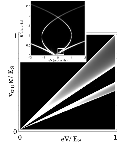
FIG. 1.: Density plot of the absolute value of the differential tunneling conductance as function of voltage $V$ and magnetic field in the absence of charging effects. The main figure is the enlargement of the region indicated by a square in the inset. The origin coincides with the resonance point $\kappa\equiv\kappa_{++}=0$ [see Eq. (1)] where Fermi points for right-movers in the two wires overlap. Velocity parameters are chosen such that $v_{\rho\text{U}}/v_{\sigma\text{U}}=1.5$, $v_{\sigma\text{L}}/v_{\sigma\text{U}}=2$, $v_{\rho\text{L}}/v_{\sigma\text{U}}=2.5$, and inter-wire interactions are neglected. The energy scale $E_{\text{s}}$ is arbitrary. Slopes of strong (bright) features are equal to the inverse of the velocity ratios given above.

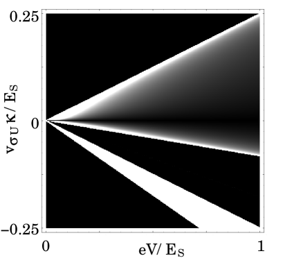
FIG. 2.: Density plot of the differential tunneling conductance for the band-filling limit. Parameters are the same as in Fig. 1. Maxima follow the slopes $\pm\frac{1}{2}\left(1-\frac{v_{\sigma\text{U}}}{v_{\sigma\text{L}}}\right)$, $\frac{v_{\sigma\text{U}}}{v_{\rho\text{U}}}-\frac{1}{2}\left(1+\frac{v_{\sigma\text{U}}}{v_{\sigma\text{L}}}\right)$, and, $\frac{v_{\sigma\text{U}}}{v_{\rho\text{L}}}-\frac{1}{2}\left(1+\frac{v_{\sigma\text{U}}}{v_{\sigma\text{L}}}\right)$, respectively. Note that, for any choice of velocities, there is at least one maximum following a negative slope.

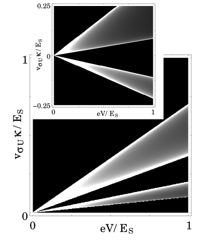
FIG. 3.: Density plot of the absolute value of the differential tunneling conductance for an intermediate situation where the applied voltage both shifts and fills electron bands. In the main figure, we have chosen $\nu_{\text{U}}=\nu_{\text{L}}=0.6$, in addition to parameters used in Fig. 1. Note that the slopes of bright maxima are suppressed from their value in the band-shifting case. The inset shows the result for the same system with finite inter-wire interactions $U_{\text{UL}}/(\pi\hbar v_{\sigma\text{U}})=0.25$ present and band-shifting parameters $\nu_{\text{U}}=0.25$, $\nu_{\text{L}}=0.05$ calculated according to Eq. (12).

REFERENCES

• [1] For a recent review, see J. Voit, Rep. Prog. Phys. 57, 977 (1994).
• [2] F. D. M. Haldane, J. Phys. C 14, 2585 (1981).
• [3] At small wave vectors, the dispersion of the phonon modes is linear for screened Coulomb interactions that we expect to be present in real quasi-1D samples.
• [4] G. D. Mahan, Many-Particle Physics (Plenum Press, New York, 1990).
• [5] V. Meden and K. Schönhammer, Phys. Rev. B 46, 15753 (1992).
• [6] J. Voit, Phys. Rev. B 47, 6740 (1993).
• [7] In addition to spin-charge separation, a Luttinger liquid can exhibit power-law behavior of electronic correlation functions. As will become clear below, we focus here entirely on effects due to spin-charge separation, using a model for a Luttinger liquid exhibiting no anomalous correlation-function exponents.
• [8] B. Dardel, D. Malterre, M. Grioni, P. Weibel, Y. Baer, and F. Lévy, Phys. Rev. Lett. 67, 3144 (1991); C. Kim, A. Y. Matsuura, Z.-X. Shen, N. Motoyama, H. Eisaki, S. Uchida, T. Tohyama, and S. Maekawa, Phys. Rev. Lett. 77, 4054 (1996); D. Orgad, S. A. Kivelson, E. W. Carlson, V. J. Emery, X. J. Zhou, and Z. X. Shen, Phys. Rev. Lett. 86, 4362 (2001).
• [9] A. Altland, C. H. W. Barnes, F. W. L. Hekking, and A. J. Schofield, Phys. Rev. Lett. 83, 1203 (1999)
• [10] D. Carpentier, C. Peça, and L. Balents, cond-mat/0103193.
• [11] O. M. Auslaender, A. Yacoby, R. de Picciotto, K. W. Baldwin, L. N. Pfeiffer, and K. West, Science 295, 825 (2002).
• [12] Momentum-resolved tunneling between low-dimensional electron systems has been used before to measure single-electron properties. For 2D–to–2D tunneling, see, e.g., J. P. Eisenstein, T. J. Gramila, L. N. Pfeiffer, and K. W. West, Phys. Rev. B 44, 6511 (1991); L. Zheng and A. H. MacDonald, Phys. Rev. B 47, 10619 (1993). Studies of 1D–to–2D tunneling can be found in B. Kardynał, C. H. W. Barnes, E. H. Linfield, D. A. Ritchie, J. T. Nicholls, K. M. Brown, G. A. C. Jones, and M. Pepper, Phys. Rev. B 55, R1966 (1997); Ref. [9]; M. Governale, M. Grifoni, and G. Schön, Phys. Rev. B 62, 15996 (2000).
• [13] D. Boese, M. Governale, A. Rosch, and U. Zülicke, Phys. Rev. B 64, 085315 (2001).
• [14] In a generic Luttinger liquid, these resonances will be suppressed due to vanishing spectral weight at the Fermi energy.
• [15] M. Büttiker, H. Thomas, and A. Prêtre, Phys. Lett. A 180, 364 (1993); M. Büttiker, J. Phys.: Condens. Matter 5, 9361 (1993); M. Büttiker and T. Christen, in: Mesoscopic Electron Transport, edited by L. L. Sohn, L. P. Kouwenhoven, and G. Schön (Kluwer Academic, Dordrecht, 1997), pp. 259-289.
• [16] Related work[10] has considered tunneling close to a resonance point with $\alpha=-\alpha^{\prime}$, neglecting any charging effects.
• [17] In addition to the four maxima exhibited in the chiral model, typically less pronounced shadow maxima can appear when non-chiral interactions are present. See, e.g., Ref. [10].
• [18] See, e.g., E. Arrigoni, Phys. Rev. Lett. 83, 128 (1999), and Ref. [10]. For the model of a Luttinger liquid considered here, exhibiting spin-charge separation but no anomalous power laws, the energy scale below which perturbation theory breaks down is given, as in the noninteracting limit, by the tunneling strength $|t|$.
• [19] J. A. del Alamo and C. C. Eugster, Appl. Phys. Lett. 56, 78 (1990).
• [20] A. M. Finkel’stein and A. I. Larkin, Phys. Rev. B 47, 10461 (1993).
• [21] M. Fabrizio and A. Parola, Phys. Rev. Lett. 70, 226 (1993); M. Fabrizio, Phys. Rev. B 48, 15838 (1993).
• [22] H. Lin, L. Balents, and M. P. A. Fisher, Phys. Rev. B 58, 1794 (1998).
• [23] J. D. Naud, L. P. Pryadko, and S. L. Sondhi, Nucl. Phys. B 565, 572 (2000); Phys. Rev. B 63, 115301 (2001).
• [24] Here we neglect Zeeman splitting which is typically small for magnetic fields needed to tune into the resonance point with $\alpha=\alpha^{\prime}=+$. It can be included straightforwardly, and one of its effects is a doubling of features in the DTC. See, e.g., S. Rabello and Q. Si, cond-mat/0008065, and Ref. [10].
• [25] We assume that tunneling is not strong enough to require a self-consistent treatment of charging effects in the wires.
• [26] Tunnel-coupled edge channels in quantum-Hall bilayers with each layer having a fractional filling factor $\leq 1$ have been considered in Ref. [23].
• [27] Y. M. Blanter, F. W. J. Hekking, and M. Büttiker, Phys. Rev. Lett. 81, 1925 (1998); R. Egger and H. Grabert, Phys. Rev. B 55, 9929 (1997), ibid. 58, 13275(E) (1998).
• [28] The validity of Eqs. (II B) was established by direct comparison with our numerical results.
• [29] J. von Delft and H. Schoeller, Ann. Phys. (Leipzig) 7, 225 (1999); and references therein.
• [30] L. S. Levitov and A. V. Shytov, cond-mat/9510006 (unpublished).
• [31] This is true within our chiral model where interactions between right-movers and left-movers are excluded. Taking them into account introduces interaction terms of the kind $\chi_{j}^{(\alpha)}\chi_{k}^{(\alpha)}\chi_{j}^{(-\alpha)}\chi_{k}^{(-\alpha)}$ that can be treated, e.g., using mean-field theory.
• [32] The reader be advised of our double use of the symbol $\tau$ as an imaginary time in Sec. II A and a real time in Sec. III B and Appendix B.
• [33] The difference $\bar{v}-v_{\sigma}=(v_{\rho-}-v_{\sigma})\frac{v_{\sigma}}{(v_{\rho-}+v_{\sigma})}$ should be large enough to enable observation in realistic systems[11] where $v_{\rho-}$ is expected to be bigger but of the same order as $v_{\sigma}$.
Refer to caption