Branched Growth with $\eta\approx 4$ Walkers

Abstract

Diffusion-limited aggregation has a natural generalization to the “$\eta$-models”, in which $\eta$ random walkers must arrive at a point on the cluster surface in order for growth to occur. It has recently been proposed that in spatial dimensionality $d=2$, there is an upper critical $\eta_{c}=4$ above which the fractal dimensionality of the clusters is $D=1$. I compute the first order correction to $D$ for $\eta<4$, obtaining $D=1+\frac{1}{2}(4-\eta)$. The methods used can also determine multifractal dimensions to first order in $4-\eta$.

The formation of patterns in nature is often controlled by diffusive phenomena. The branching of a less viscous fluid such as water injected into a more viscous fluid such as oil, the dendritic complexity of a snowflake, or the formation of veins of metals on the surface of certain rocks, all display pattern formation processes controlled by the diffusive transport of some quantity[1].

The simplest model for diffusion-controlled growth was introduced twenty years ago by Witten and Sander[2]. Their model of “diffusion-limited aggregation” (DLA) describes the formation of an aggregate by sequential deposition of randomly walking particles arriving from infinity. There is an electrostatic formulation of this process, in which the $n$-particle cluster is chosen as an equipotential of a Laplacian field, which has a source at infinity. The local growth probability, i.e., the probability of deposition of the $n+1$’st particle, is then chosen proportional to the local electric field on the surface of the cluster.

A natural generalization of this model is to fix the growth probability on the surface proportional to the $\eta$’th power of the local electric field. This corresponds to a random walk model in which $\eta$ independent walkers must arrive at the same surface point in order for growth to occur at that point. These “$\eta$-models” were originally introduced by Niemeyer et al. as models for dielectric breakdown, and represent a useful formal extension of DLA[3].

These models were used in an important recent work of Hastings to propose a systematic perturbative approach to DLA[4]. This work argued that the fractal dimension $D$ of $\eta$-model clusters collapses to $D=1$ in spatial dimensionality $d=2$ for $\eta\geq 4$, and that this value of $\eta_{c}=4$ therefore represents an upper critical $\eta$ for these models. Dimensions and other properties of models for $\eta<4$ can then be determined by perturbative renormalization in $4-\eta$. The case of DLA ($\eta=1$) is in principle accessible, although satisfactory agreement with the numerical result $D=1.71$ may be difficult to achieve given the large value of $4-\eta$ required. However, considerable computational difficulties arose in implementing this program. Nevertheless, rough numerical results for the first order correction to $D$ were obtained, which agree with the exact result expressed in Eq. (1) below.

Many of the ideas used by Hastings originated in the “branched growth model,” a phenomenological treatment of DLA proposed a number of years ago by my collaborators and myself[5]. The purpose of the current work is to show that the branched growth model actually allows easy computation of perturbative terms, at least to first order in $4-\eta$. This ease can be understood as a consequence of the branched growth model becoming exact as one approaches $\eta=4$. In particular, I obtain the result that the dimension $D$ is given to first order in $4-\eta\geq 0$ by

$$D=1+\frac{1}{2}(4-\eta)+O(4-\eta)^{2}.$$ (1)

I obtain as well first order expressions for the multifractal dimensions of the growth measure.

In this work, I will first review the salient features of the branched growth model, and I will argue that to lowest order in $4-\eta$ it well represents the dynamics of the underlying Laplacian growth process. I compute the dimensions of the clusters by two different means, and show that both methods give Eq. (1). I then derive an integral formula for the multifractal dimensions to $O(4-\eta)$, and give a simple approximation to the actual values of these dimensions at this order. Finally, I discuss prospects for extending this computation to higher orders in $4-\eta$.

The branched growth model places a fundamental importance on the microscopic process of tip-splitting, whereby a growing branch forks into two growing branches. This process occurs at a microscopic scale, on the order of the particle size or cutoff $a$ in dimension. Thus the frequency and detailed dynamics of tip-splitting is controlled by microscopic and presumably non-universal details of the way particles attach at or near the tip of a growing branch. We regard tip-splitting as the fundamental stochastic process in the model; we disregard all other forms of stochasticity such as the “shot noise,” i.e., the purely statistical variations in the number of particles depositing at different positions in the cluster. The reader should note that the precise role of stochasticity in DLA has recently been quite controversial[6]; although we believe that the theory to be outlined in this work is stable against obvious additional sources of stochasticity such as shot noise, a complete understanding of the roles of different kinds of noise requires more systematic study.

Once a branch splits into two, we follow its additional development by implementing a deterministic version of the $\eta$-model growth rule. Near the tip of a linear equipotential, the electric field in two dimensions diverges as

$$E(w)\sim w^{-1/2}$$ (2)

with $w$ the distance from the tip. Thus, for $\eta>2$ the growth measure, which is proportional to $E^{\eta}(w)$, is entirely dominated by growth at the tips. Since we work near $\eta=4$, we need only follow the progress of the tips in the deterministic portions of the growth, as well as keeping track of the generation of new tips through (stochastic) tip-splitting.

Consider two branches emanating from the same tip-splitting event. The masses (particle numbers) of the two branches we will write as $n_{L}$ for the left-hand branch, and $n_{R}$ for the right-hand branch; the growth measures of the left-hand and right-hand branches we write as $p_{L}$, $p_{R}$ respectively. Defining relative growth rate and mass parameters $x$ and $y$ respectively by

$$x=\frac{p_{L}}{p_{L}+p_{R}},$$ (3)

and

$$y=\frac{n_{L}}{n_{L}+n_{R}}\equiv\frac{n_{L}}{n_{T}},$$ (4)

with $n_{T}=n_{L}+n_{R}$, we see by elementary manipulations that

$$\frac{dy}{d{\rm log}(n_{T})}=x-y.$$ (5)

In principle, we can define a function $G$ of the overall cluster geometry such that

$$\frac{dx}{d{\rm log}(n_{T})}=G.$$ (6)

In the branched growth model, $G$ is taken to be a function of $x$ and $y$ alone.

Let us consider a growing fork, i.e., a branch with equal sub-branches (the tines of the fork) immediately after tip-splitting. It is convenient to describe the fork by the conformal map $w=F(z)$ that maps the real axis in the $z$-plane onto the fork in the physical $w$-plane; $|dw/dz|^{-1}$ gives the local electric field at $w$. If we choose a fork for which the angle between the tines is $\theta_{1}$, the map is given by

$$w=F(z)=z^{\alpha_{1}}(z^{2}-1)^{\alpha_{2}}$$ (7)

with $\alpha_{1}=\theta_{1}/\pi$ and $\alpha_{2}=1-(\theta_{1}/2\pi)$, where the constant $1$ is chosen arbitrarily. The derivative of the map $F^{\prime}(z)$ possesses zeroes at $z_{\pm}=\pm\sqrt{\alpha_{1}/2}$, which correspond to the points of the fork. We can fix $\alpha_{1}$ by requiring that the points are oriented towards the maximum field, so that the fork geometry is unchanged by the growth process; this requires that

$$\frac{d}{dz}\left(\frac{F^{\prime}(z)}{z-z_{+})}\right)|_{z=z_{+}}=\frac{d}{dz}\left(\frac{F^{\prime}(z)}{z-z_{-})}\right)|_{z=z_{-}}=0$$ (8)

which after some algebra determines $\alpha_{1}=\frac{2}{5}$ or $\theta_{1}=\frac{2}{5}\pi$ [4, 7].

The competition between the two growing tines of the fork is intrinsically unstable. A simple computation shows that the eigenvalue of the instability is [4]

$$\nu=\frac{\eta}{2}-1.$$ (9)

Since the two tines are supposed to be created with approximately constant probability to be found near the fixed point $(x,y)=(\frac{1}{2},\frac{1}{2})$, the eigenvalue of the instability can be related to the probability that the branch pair is still active (i.e., one branch has not been entirely screened by the other) as $n_{T}$ grows; this probability is $P\propto n_{T}^{-\nu}$. Since for a main branch of length $r$ there will have been $O(r)$ opportunities to branch, requiring that $O(1)$ sidebranch always be active implies $\nu=D^{-1}$ [5], which already suggests Eq. (1). However, it is productive to consider this question in more detail.

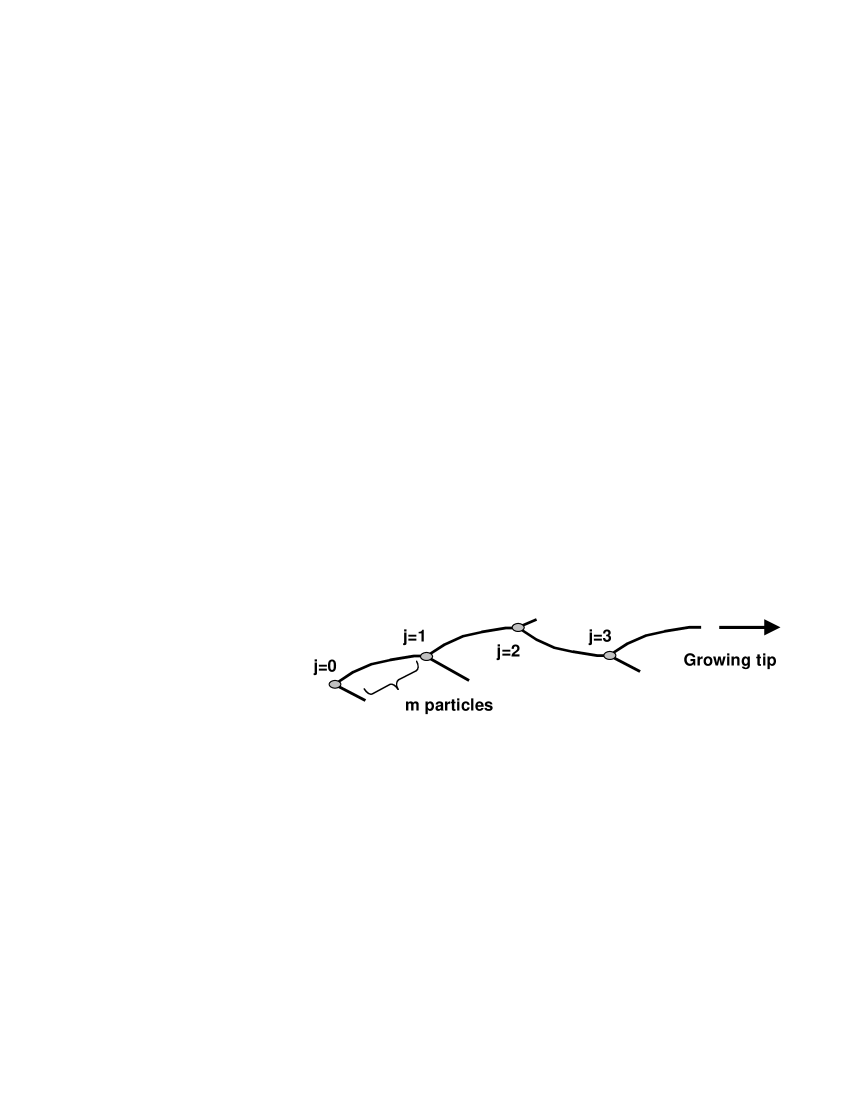
FIG. 1.: The geometry of the growing branch. After each tip-splitting event, the weaker branch is screened by the stronger. The tip-splittings are indexed by $j\geq 0$. Tip-splittings are separated by $m$ particles on the main branch.

Consider a growing branch of $n$ particles, which tip-splits every $m\ll n$ particles. The side-branches thus generated persist for a certain distance, and are then screened by the main branch. Index these tip-splittings by $0\leq j\leq J$ (see Figure 1). Then at each $j$ there can be defined parameters $x_{j}$, $y_{j}$, and $n_{j,T}$, giving the relative mass and growth probabilities of the side-branches, as well as the total mass of the remainder of the main branch plus the side-branch in question (the total mass to the right of the branch point in Figure 1). We choose our definition of “left” and “right” in Eqs.  (3-4) so that each $x_{j}\leq\frac{1}{2}$. The growth rate at the overall tip is then given by

$$p_{tip}=\prod_{j=0}^{J}(1-x_{j}).$$ (10)

Suppose that at the $j$’th branching, the initial value of $x_{j}$ is given by

$$x_{j}(n_{j,T}=1)=\frac{1}{2}-\varepsilon_{j}^{\nu},$$ (11)

defining a random variable for the branching $\varepsilon_{j}$. The distribution of $\varepsilon$, $\rho(\varepsilon)$, is chosen so that $x_{j}$ does not have any singularity in its initial distribution near $x=1/2$–this reflects the microscopic origin of the stochasticity.

$$\lim_{\varepsilon\to 0}\rho(\varepsilon)=\rho_{0}\varepsilon^{\nu-1},$$ (12)

with the large $\varepsilon$ behavior constrained by the integrability of $\rho(\varepsilon)$. In the branched growth model, the dependence of $x_{j}$ on $n_{j,T}$ and $\varepsilon_{j}$ at each branching point is the same; we now assume this to be the case in this more general model as well. The argument below will establish that this assumption is correct to lowest order in $4-\eta$.

If the dynamics of each branching point are the same, then there must exist some $G(x,y)$ in Eq. (6). The values of $x$ and $y$ can then be integrated to obtain $x(h)$, $y(h)$ from Eqs. (5-6), with $h\propto n_{T}$ and $(x(0),y(0))=(\frac{1}{2},\frac{1}{2})$. Note that this choice of variables means that the dependence of $x$ on $\varepsilon$ can be encoded by

$$x(n_{T},\varepsilon)\approx x(\varepsilon n_{T}\equiv h),$$ (13)

and similarly for $y$. This formula becomes exact for $n_{T}$ large.

We can now see that to $O(\rho_{0})$

$$\langle p_{tip}\rangle=1-\sum_{j}\langle x_{j}\rangle=1-\sum_{j=0}\int d\varepsilon\rho_{o}\varepsilon^{\nu-1}x(\varepsilon n_{j,T}),$$ (14)

or, extracting the dependence on $\{n_{j,T}\}$ from the integrals,

$$\langle p_{tip}\rangle=1-\sum_{j}\langle n_{j,T}^{-\nu}\rangle\left(\rho_{0}\int_{0}^{\infty}dh\;h^{\nu-1}x(h)\right).$$ (15)

To evaluate $\sum_{j=0}\langle n_{j,T}^{-\nu}\rangle$, we use a simple trick. Let us first assume that

$$\sum_{j=0}\langle n_{j,T}^{-\nu}\rangle=\lambda{\rm log}n.$$ (16)

We will now confirm this form, and compute the parameter $\lambda$. Consider the second branching at $j=1$. We have

$$\lambda{\rm log}n=\frac{1}{n^{\nu}}+\sum_{j=1}\langle n_{j,T}^{-\nu}\rangle=\frac{1}{n^{\nu}}+\langle\lambda{\rm log}\left[(1-y_{0})n-m\right]\rangle,$$ (17)

since the number of particles in the main branch below the second sidebranching is $n_{1}=(1-y_{0})n_{0}-m$ (see Figure 1). Note that $n\equiv n_{0,T}$. This leads to

$$\frac{1}{n^{\nu}}=-\frac{\rho_{0}}{n^{\nu}}\lambda\int_{0}^{\infty}dh\;h^{\nu-1}{\rm log}(1-y(h))+\frac{\lambda m}{n}\langle(1-y_{0})^{-1}\rangle.$$ (18)

As $h\to\infty$, the weaker branch will die at some fixed mass and $y(h)\to\bar{h}/h$. Thus as $\nu\to 1$, the integral over $h$ on the right-hand side of Eq. (18) diverges as

$$\int dh\;h^{\nu-1}{\rm log}(1-y(h))=-\frac{\bar{h}}{1-\nu}+O(1)$$ (19)

Thus we obtain immediately

$$\lambda=\frac{1-\nu}{\bar{h}\rho_{0}}+O(1-\nu)^{2}$$ (20)

so that the sum in Eq. (15) is $O(1-\nu)=O(4-\eta)$.

The fact that this “propagator” sum is $\propto(1-\nu){\rm log}n$ is the key formal result of this work, which allows us to construct a direct renormalization group for the dimension and other properties of the $\eta$-models. The procedure, in principle, is as follows. First, a naive perturbative expansion in $\rho_{0}$ is constructed, along the lines of ref. [8]. The computation above shows an example to first order in $\rho_{0}$. This expansion should account both for the different contributions of the various tips to the quantity being computed, as well as the influence of the internal structure of the various branches on the functions $x(h)$, $y(h)$. In this expansion, sums over $\langle n_{j,T}^{-\nu}\rangle$ such as that appearing in Eq. (15) will appear, as well as more complex, albeit still ultimately logarithmic, sums. Performing these sums, one will replace the original series in $\rho_{0}$ with a logarithmic series in $1-\nu$. The methods of ref. [8] easily show that the higher order terms in $\rho_{0}$ will be higher order in $1-\nu$ upon computation of these sums. This series then forms the basis of a direct renormalization calculation of the quantity of interest.

We illustrate this by returning to the growth rate of the overall branch tip. To zeroth order in $1-\nu$, we can represent the structure of the two branches, which we use to compute $x(h)$ and $y(h)$, by a fork with two growth sites at the fork tips. Thus we generalize the fork with equal-length tines to a fork which may grow different lengths on the two sides–in so doing, there will be a tendency for the two sides to curve away from being perfectly straight and separated by an angle $\theta_{1}$, as shown in Figure 1. Standard techniques of integrating the conformal map for Laplacian growth structures will suffice for determining the full $x(h)$ and $y(h)$ for this case[9]; below we give a simple approximation to these quantities. To this order, there are no additional variables describing the internal structure of the branches, so we are justified in assuming the same $x(h)$ and $y(h)$ at each branch point.

However, it turns out that we need not compute $x(h)$ or $y(h)$ explicitly in order to compute the first order correction to the tip growth rate. From the definitions of $x(h)$ and $y(h)$, we have that

$$\frac{d(yn_{T})}{dn_{T}}=x,$$ (21)

implying by integration of parts that

$$\int_{0}^{\infty}dh\;h^{\nu-1}x(h)=(1-\nu)\int_{0}^{\infty}dh\;h^{\nu-1}y(h).$$ (22)

The divergence of $\int dhh^{\nu-1}{\rm log}(1-y(h))$ as $\nu\to 1$ originates from large values of $h$, or small values of $y$. Thus to lowest order in $1-\nu$ we have

$$\int_{0}^{\infty}dh\;h^{\nu-1}{\rm log}(1-y(h))=-\int_{0}^{\infty}dh\;h^{\nu-1}y(h),$$ (23)

and

$$\sum_{j}\langle n_{j,T}^{-\nu}\rangle\rho_{0}\int_{0}^{\infty}dh\;h^{\nu-1}x(h)=\frac{\rho_{0}\int_{0}^{\infty}dh\;h^{\nu-1}x(h)}{\rho_{0}\int_{0}^{\infty}dh\;h^{\nu-1}y(h)}{\rm log}n=(1-\nu){\rm log}n,$$ (24)

so that

$$p_{tip}=1-(1-\nu){\rm log}n+O(1-\nu)^{2}.$$ (25)

Since we expect $p_{tip}\propto n^{D^{-1}-1}$, with $D$ mass-radius scaling dimension [10], this implies with Eq. (9) that

$$D=1+\frac{1}{2}(4-\eta)+O(4-\eta)^{2},$$ (26)

as advertised.

To compute multifractal dimensions to $O(4-\eta)$, I use similar techniques. Following ref. [8], and using $i$ as an index to growth tips, we see that the multifractal spectrum $\sigma(q)$ for the growth measure (not the harmonic measure) is given by

$$\langle\sum_{i}p_{i}^{q}\rangle\equiv n^{-\sigma(q)}=1+\lambda{\rm log}n\left\{\int_{0}^{\infty}dh\left[x^{q}(h)+(1-x(h))^{q}-1\right]\right\}+O(1-\nu)^{2},$$ (27)

yielding

$$\sigma(q)=-\frac{1-\nu}{\bar{h}}\left\{\int_{0}^{\infty}dh\left[x^{q}(h)+(1-x(h))^{q}-1\right]\right\}+O(1-\nu)^{2}.$$ (28)

To obtain explicit results for the multifractal dimensions, we need the trajectories $x(h)$ and $y(h)$. I use a simple artifice that gives a useful approximation to this trajectory. The integral in Eq. (28) is dominated by values of $x$ near $x=\frac{1}{2}$. We can thus approximate the integral by taking the linear trajectory in the $x-y$ plane near the center $(x,y)=(\frac{1}{2},\frac{1}{2})$ and extending it to the boundaries $x=0,1$. (This approximation is referred to as “model Z” in ref. [5].) Explicitly, we write, taking the lowest order $\nu=1$,

$$x(h)=\cases{\frac{1}{2}-h,&if $h<\frac{1}{2}$\cr 0,&if $h\geq\frac{1}{2},$\cr}$$ (29)

and

$$y(h)=\cases{\frac{1}{2}-\frac{1}{2}h,&if $h<\frac{1}{2}$,\cr 1/8h,&if $h\geq\frac{1}{2}$ .\cr}$$ (30)

which agrees with Eq. (5).

The approximate result for the multifractal dimensions is then

$$\sigma(q)=2(4-\eta)\frac{q-1}{q+1}+O(4-\eta)^{2}.$$ (31)

Note that due to our total suppression of non-growing portions of the measure, we do not recover the identity $\sigma(0)=-D$.

The extension of these results to higher orders in $4-\eta$, and in particular to the case of DLA ($\eta=1$), will require some further formal development. Reference [8] successfully computes the most divergent and next-most divergent terms at all orders in $\rho_{0}$ for the multifractal dimensions for the branched growth model; the behavior of the higher order logarithms in this case does allow resummation of the theory for, e.g., quenched and annealed multifractal dimensions. In our case, we need to add a family of terms representing the deviations from the perfect branched growth model behavior, which arise from fluctuations in the internal structure of the branches. Fortunately, there are indications that these fluctuations are also renormalizable [5].

I am grateful to M.B. Hastings for drawing my attention to ref. [4], and for a critical reading of this manuscript.

REFERENCES

- [1] T.C. Halsey, Physics Today 53, 11:36 (November 2000); and references therein.
- [2] T. A. Witten and L. M. Sander, Phys. Rev. Lett. 47, 1400 (1981).
- [3] L. Niemeyer, L. Pietronero, and H. J. Wiesmann, Phys. Rev. Lett. 52, 1033 (1984).
- [4] M.B. Hastings, cond-mat/0104344.
- [5] T. C. Halsey, Phys. Rev. Lett 72, 1228 (1994); T. C. Halsey and M. Leibig, Phys. Rev. A 46, 7793 (1992).
- [6] B. Davidovitch, M.J. Feigenbaum, H.G.E. Hentschel, and I. Procaccia, Phys. Rev. E 62 1706 (2000).
- [7] T.C. Halsey, B. Shaw, and M. Leibig, unpublished.
- [8] T.C. Halsey, K. Honda, and B. Duplantier, J. Stat. Phys. 85, 681 (1996); T. C. Halsey, B. Duplantier, and K. Honda, Phys. Rev. Lett. 78, 1719 (1997).
- [9] M. B. Hastings and L. S. Levitov, Physica D 116, 244 (1998); B. Davidovich et. al., Phys. Rev. E 59, 1368 (1999).
- [10] L. A. Turkevich and H. Scher, Phys. Rev. Lett. 55, 1026 (1985).