[

Collective dynamics of two-mode stochastic oscillators

Abstract

We study a system of two-mode stochastic oscillators coupled through their collective output. As a function of a relevant parameter four qualitatively distinct regimes of collective behavior are observed. In an extended region of the parameter space the periodicity of the collective output is enhanced by the considered coupling. This system can be used as a new model to describe synchronization-like phenomena in systems of units with two or more oscillation modes. The model can also explain how periodic dynamics can be generated by coupling largely stochastic units. Similar systems could be responsible for the emergence of rhythmic behavior in complex biological or sociological systems.

(Last revised )

]

Collective dynamics of stochastic systems shows a great variety of interesting phenomena like pulsating patterns [2], spiral waves [3], synchronization [4] or stochastic resonance [5]. While the collective dynamics of single mode stochastic oscillators is relatively well understood [6], the dynamics of stochastic oscillators with many possible modes is less studied [7], and leads to interesting and new effects. An example in this sense is our recent study on the peculiar dynamics of the rhythmic applause [8], where the fascinating dynamics appears as a result of two different frequency clapping modes [9]. Many other biological or physical systems exist, which perform stochastic oscillations with different modes. As examples we mention the unicellular alga Gonyaulax polyedra where circadian oscillators with two different periods have been shown to co-exist [10], the thalamocortical relay neurons which can generate either spindle (7-14 Hz) or delta (0.5-4 Hz) oscillations [11], and the hippocampal CA3 model which spontaneously can generate four different rhythms [12]. When the system can switch between the available modes as a function of some threshold condition, new and interesting collective behavior is observed.

The present study reports on such results for an ensemble of coupled two-mode stochastic oscillators. As a function of a threshold condition we reveal different type of synchronized and unsynchronized phases. We also show that rhythmic collective behavior can be generated by suitably coupling largely stochastic units, i.e. the periodicity of the total output relative to the output of one stochastic oscillator can be strongly enhanced. As an immediate application we offer a new and realistic description for the dynamics of the rhythmic applause, reproducing all experimentally observed characteristics.

Our system is composed by identical pulse-coupled two-mode stochastic oscillators. Their cycle can be performed in two modes: $A\rightarrow B_{I}\rightarrow C\rightarrow A$ or $A\rightarrow B_{II}\rightarrow C\rightarrow A$, respectively. The periods corresponding to these two modes $T_{I}$ and $T_{II}$ are given as $T_{I}=\tau_{A}+\tau_{B_{I}}+\tau_{C}$ and $T_{II}=\tau_{A}+\tau_{B_{II}}+\tau_{C}$, where $\tau_{A}$, $\tau_{B}$ and $\tau_{C}$ are time intervals spent in state $A$, $B$ and $C$, respectively. The stochastic part of the dynamics is state A, and $\tau_{A}$ is a stochastic variable with distribution:

$$P(\tau_{A})=\frac{1}{\tau^{*}}exp(-\frac{\tau_{A}}{\tau^{*}}),$$ (1)

($\tau^{*}=\langle\tau_{A}\rangle$). State $A$ should be imagined and modeled with an escape dynamics of a stochastic field-driven particle from a potential valley of depth $U$. If the stochastic force-field is totally uncorrelated with $\langle\xi\rangle=0$ and $\langle\xi(t)\xi(t+\tau)\rangle=D\delta(\tau)$ we get a distribution of escape times given in (1) with: $\tau^{*}\sim exp(U/D)$. In analogy with the well-known FitzHugh-Nagumo system [13], state $A$ corresponds to a stochastic reaction time of the neuron fire. This causes all the experimentally observed fluctuations in the rhythmic human activities [14, 15]. In state $B$ and $C$ the dynamics is deterministic, and corresponds to the relaxation of the neurons [14, 16]. State B represents a ”waiting time” or the rhythm giving part of the cycle. In biological systems this is a period the individual units want to impose, and usually this is the longest part of the cycle. The length of state B ($\tau_{B_{I}}$ or $\tau_{B_{II}}$) distinguishes between the two modes. We have chosen $\tau_{B_{II}}=2\tau_{B_{I}}$. The output of the units is in state C. During this state the oscillator emits a constant intensity pulse of strength $1/N$ where $N$ is the number of oscillators in the system. The output of the whole system at a given moment is

$$f=\sum_{i=1}^{N}f_{i},$$ (2)

where $f_{i}$ is the output of oscillator $i$, $f_{i}=1/N$ if the given oscillator is in state $C$ and $f_{i}=0$ otherwise. This total output is the origin of the coupling and shifts the oscillators between their operating modes. The rules for the evolution of the system are as follows: (i) oscillators start with randomly selected modes and phases and follow the stated dynamics; (ii) there is a fixed output intensity, $f^{*}$, for the system; (iii) after completing the dynamics in state $A$, each oscillator will choose to operate either in mode I or mode II; (iv) if at that moment $f<f^{*}$ the oscillator will operate in mode I, otherwise will follow mode II. The above dynamics has the tendency to keep the average total output as close as possible to $f^{*}$. Since each oscillator has a fixed output intensity, this can be achieved only through switching between the available modes. In this sense the proposed rules are natural, making our model realistic.

The evolution of a single uncoupled unit is simple since it preserves the starting mode ($s$). The average value of its period is:

$$\langle T\rangle=\langle\tau_{A}+\tau_{B_{s}}+\tau_{C}\rangle=\tau^{*}+\tau_{B_{s}}+\tau_{C}.$$ (3)

Its relative standard deviation

$$R=\frac{\sqrt{\langle T^{2}\rangle-\langle T\rangle^{2}}}{\langle T\rangle}=\frac{\tau^{*}}{\tau^{*}+\tau_{B_{s}}+\tau_{C}},$$ (4)

shows an increasing tendency as a function of $\tau^{*}$.

In contrast with the simple uncoupled case, the dynamics of the coupled units is complex. Generally the oscillators will shift irregularly between their two modes. As a function of $f^{*}$ many interesting regimes are observed.

For the limiting values $f^{*}=0$ or $1$ the dynamics is trivial. For $f^{*}=1$ we always have $f<f^{*}$ and all units operate in mode I. The $f$ output randomly fluctuates due to both the initial random phases and the stochastic nature of $\tau_{A}$. As the number of units increases, the variance of this fluctuation decreases. The average value of the collective output $\langle f(f^{*}=1)\rangle=\langle f\rangle_{1}$, is a function of $\tau_{C}$ and $\langle T_{I}\rangle$ only:

$$\langle f\rangle_{1}=\frac{\tau_{C}}{\langle T_{I}\rangle}.$$ (5)

The above considerations will apply in the $N>>1$ limit for the $f^{*}>\langle f\rangle_{1}$ cases as well. In this manner we can analytically predict that for high enough $f^{*}$ values the units operate as simple uncoupled stochastic oscillators in mode I. For $f^{*}\leq 0$ all units operate in mode II, and again there is no effective coupling between the units. The total signal will randomly fluctuate, and due to the larger $\langle T_{II}\rangle$ value its mean will be smaller than the one measured in the $f^{*}>\langle f\rangle_{1}$ cases:

$$\langle f\rangle_{0}=\langle f(f^{*}=0)\rangle=\frac{\tau_{C}}{\langle T_{II}\rangle}<\langle f\rangle_{1}$$ (6)

For $0<f^{*}<\langle f\rangle_{1}$ we have a nontrivial regime, where the coupling is effective and the oscillators switch between their modes. This region will be studied by computer simulations. We can numerically follow both the dynamics of a selected unit and the total $f$ output of the system. For fixed $\tau_{B_{I}}$, $\tau_{B_{II}}$ and $\tau_{C}$ values the parameters governing the system dynamics are $f^{*}$ and $\tau^{*}$. We choose $\tau_{B_{I}}=0.4$ and $\tau_{C}=0.1$. By mapping the relevant $\{f^{*},\tau^{*}\}$ parameter-space, four different regimes (phases) can be revealed. Phase I, is an unsynchronized regime with $\langle f\rangle=\langle f\rangle_{0}$ (Fig. 1a). Phase II, is a synchronized regime with quasi-periodic total output and large oscillation periods close to the $\langle T_{II}\rangle$ value (Fig. 1b). Phase III, is a synchronized regime with quasi-periodic output and slow oscillation periods close to the $\langle T_{I}\rangle$ value (Fig. 1c). Phase IV, is an unsynchronized regime with $\langle f\rangle=\langle f\rangle_{1}$ (Fig. 1d).

Changing the values of $\tau_{B}$ and $\tau_{C}$ leads to qualitatively similar phases in the parameter space. From the phase-space sketched in Fig.2 we learn that by increasing the value of $f^{*}$ the systems collective output changes from the unsynchronized phase I behavior to the synchronized phase II and phase III dynamics, leading finally to the unsynchronized phase IV regime. As $\tau^{*}$ is increasing phase III disappears ($\tau^{*}\geq 0.5$) and the $f^{*}$ interval where synchronization is present (phase II and III) diminishes. In agreement with our previous analytic justifications, in phase I we have $\langle f\rangle=\langle f\rangle_{0}$ (Fig. 1a), in phase IV, $\langle f\rangle=\langle f\rangle_{1}$ and for $f^{*}>\langle f\rangle_{1}$ the collective behavior of the system always corresponds to the phase IV one.

In the $0<f^{*}<\langle f\rangle_{1}$ regime the dynamics of a single unit is non-trivial. The units stochastically shift between mode I and mode II oscillations. In this regime although the movement of each unit is largely stochastic, their collective behavior leads to a periodic output. In order to characterize numerically the enhancement in the periodicity we define a measure for it. Let us denote the output signal as a function of time as $f(t)$. We can define an error function, $\Delta(T)$, which characterizes numerically how strongly the $f(t)$ signal differs from a periodic signal with period $T$

$$\Delta(T)=\frac{1}{2M}lim_{x\rightarrow\infty}\frac{1}{x}\int_{0}^{x}\mid f(t)-f(t+T)\mid dt,$$ (7)

where

$$M=lim_{x\rightarrow\infty}\frac{1}{x}\int_{0}^{x}\mid f(t)-<f(t)>\mid dt$$ (8)

$$<f(t)>=lim_{x\rightarrow\infty}\frac{1}{x}\int_{0}^{x}f(t)dt$$ (9)

The general shape of the $\Delta(T)$ curve as a function of $T$ is sketched on Fig. 3. For any $f(t)$ oscillating function we have an initially increasing tendency at small $T$ values, after which for $T=T_{m}$ a minimum ($\Delta_{m}$) is reached. One can state that $T_{m}$ is the best approximation for the $f(t)$ signals period, and the ”periodicity level” of the signal is characterized by:

$$p=\frac{1}{\Delta_{m}}$$ (10)

We can compute this parameter both for one oscillator working independently ($p_{1}$) in the long period mode (where the effect of stochasticity on the period is smaller) and for the whole system ($p$). The ratio $p/p_{1}$ will characterize the enhancement in the periodicity. We have analyzed throughout the $\{\tau^{*},f^{*}\}$ parameter space this enhancement in the periodicity. Results for $N=200$ oscillators are given in Fig. 4. From this data it is clear that there is a quite large parameter space (corresponding to small values of $f^{*}$ and large limits for $\tau^{*}$) where the enhancement in the periodicity is considerable. The computed best periods ($T_{m}$) are in agreement with the phases previously discussed and sketched in Fig. 2. Increasing the number of coupled oscillators will further enhance the periodicity of the total output. As an example results for $\tau^{*}=0.4$ and $f^{*}=0.1$, are presented in Fig. 5. It is also interesting to note the stochastic resonance type effect [5] for the enhancement in the periodicity (Fig. 4). For fixed $f^{*}$ values there is an optimal noise level ($\tau^{*}$) in the oscillators dynamics, where a maximal $p/p_{1}$ enhancement ratio is achieved through the considered coupling.

As an immediate application one can create a new model and explanation for the phenomenon of rhythmic applause [9]. Different phases of the collective output (Fig.2) reproduces the regimes observed in collective clapping. The high intensity (phase IV) unsynchronized phase corresponds to the initial thunderous clapping of the spectators following an exceptional performance. Phase II describes the rhythmic applause where spectators clap in unison with a relatively long period. Phase III with a shorter period and partly synchronized output is characteristic for the unstable transition intervals from synchronized to unsynchronized clapping. The low intensity unsynchronized phase I dynamics is characteristic to the clapping of a non-enthusiastic audience. Modeling the clapping individuals by the proposed two-mode stochastic oscillators, and the coupling between them by the proposed threshold criteria is realistic and in agreement with experimental results: i) the clapping sound is pulse like and is reproduced by state C of the oscillators; ii) the clapping period of one individual has a fluctuating nature [15] and is modeled by state A of the dynamics; iii) the rhythm of the clapping is modeled by state B; iv) our previously reported measurements on clapping individuals [8] revealed the existence of the two distinct clapping modes with short and longer periods, respectively; v) the period of the longer clapping mode was found do be roughly two times larger than the one of the short clapping mode. In view of this new model the characteristic interplay between synchronized and unsynchronized regimes in the rhythmic applause should be a consequence of a peculiar dynamics in the $f^{*}$ threshold, and should have a psychological origin. It is clear that after a bad performance the $f^{*}$ threshold is low and leads to phase I type collective response. For an enthusiastic audience $f^{*}$ is big and high intensity collective response forms, resembling the total output of the units in phase IV. By lowering the level of $f^{*}$ (fatigue or just resting…?) synchronized collective response arises (phase III) which corresponds to the rhythmic applause.

In our opinion the presented model has possibilities for understanding and modeling the origin of other rhythmic biological or sociological phenomena [17]. The most interesting aspect of our results is the finding that regular periodic output can be obtained by coupling a large number of stochastic units. Similar phenomena should be responsible for the emergence of rhythmic behavior in complex biological or sociological systems.

The present study was done during a common fellowship at Collegium Budapest- Institute of Advanced Study (Hungary). We acknowledge the professionally motivating academic atmosphere from the Collegium.

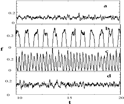
FIG. 1.: Total $f$ output of 200 coupled two-mode oscillators ($\tau^{*}=0.1$, $\tau_{B_{I}}=0.4$, $\tau_{C}=0.1$ and $f^{*}=-0.1$ (a), $f^{*}=0.1$ (b), $f^{*}=0.2$ (c), $f^{*}=0.3$ (d)).

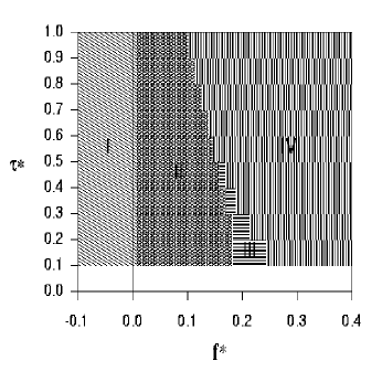
FIG. 2.: Phases in the $\{f^{*},\tau*\}$ parameter-space ($N=200$, $\tau_{B_{I}}=0.4$, $\tau_{C}=0.1$).

FIG. 3.: Characteristic shape of $\Delta(T)$. Determining the $\Delta_{m}$ and $T_{m}$ parameters. ($\tau*=0.1$, $f^{*}=0.3$, $\tau_{B_{I}}=0.4$, $\tau_{C}=0.1$, $N=200$)

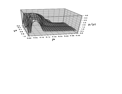
FIG. 4.: Enhancement in the periodicity ($p/p_{1}$) as a function of the $\tau^{*}$ and $f^{*}$ relevant parameters. (Results for $N=200$ oscillators, $\tau_{B_{I}}=0.4$, $\tau_{C}=0.1$)

FIG. 5.: Enhancement in the periodicity of the output ($p/p_{1}$) as a function of the number of oscillators in the system. ($f^{*}=0.1$ and $\tau^{*}=0.4$ $\tau_{B_{I}}=0.4$, $\tau_{C}=0.1$)

REFERENCES

- [1] on leave from: Babes-Bolyai University, Dept. of Theoretical Physics, str. Kogalniceanu 1, RO-3400, Cluj-Napoca, Romania. E-mail: zneda@phys.ubbcluj.ro
- [2] H. Hempel, L. Schimansky-Geier and J. Garcia-Ojalvo, Phys. Rev. Lett. 82, 3713 (1999)
- [3] P. Jung, Phys. Rev. Lett. 78, 1723 (1997); P. Jung, A. Cornell-Bell, K. Madden and F. Moss, J. Neurophysiol. 79, 1098 (1998)
- [4] A. Neiman, Phys. Rev. E 49, 3484 (1994); A. Neiman, L. Schimansky-Geier, A. Cornell-Bell and F. Moss; Phys. Rev. Lett. 83, 4896 (1999); V. Anischenko, A. Neiman, A. Silchenko and I. Khovanov, Dynamics and Stability of Systems, 14, 2111 (1999)
- [5] P. Jung and G. Mayer-Kress, Chaos 5, 458 (1995); S.K. Han, W.S. Kim and H. Kook; Phys. Rev. E 58, 2325 (1998)
- [6] W. Gerstner and J.L. van Hemmen; Phys. Rev. Lett. 71, 312 (1993); Ch. Kurrer and K. Schulten, Phys. Rev. E 51, 6213 (1995); S.K. Han, T.G. Yim, D. E. Postnov and O.V. Sosnovtseva, Phys. Rev. Lett. 83, 1771 (1999)
- [7] S.Y. Vyshkind; Radiophysics and Quantum Electronics 21, 1008 (1978)
- [8] Z. Neda, E. Ravasz, Y. Brechet, T. Vicsek and A. Barabasi, Nature 403, 849 (2000)
- [9] Z. Neda, E. Ravasz, Y. Brechet, T. Vicsek and A. Barabasi, Rhys. Rev. E 61, 6987 (2000)
- [10] D. Morse, J.W. Hastings and T. Roenneberg, J. Biol. Rhythms 9, 263 (1994)
- [11] X.J. Wang, Neuroscience 59, 21 (1994)
- [12] K. Tateno, H. Hayashi and S. Ishizuka, Neural Networks 11, 985 (1998)
- [13] A.S. Pikovsky and J. Kurths, Phys. Rev. Lett. 78, 775 (1997); B. Lindner and L. Schimansky-Geier, Phys. Rev. E 60, 7270 (1999); B. Lindner and L. Schimansky-Geier, Phys. Rev. E 61, 6103 (2000)
- [14] M.R. Rosenzweigh, A.L. Leiman and S.M. Breedlove, Biological Psychology (Sinauer Associates, Inc. Publishers, Sunderland, Massachusetts, 1996);
- [15] T. Musha, K. Katsurai and Y. Teramachi, IEEE Transactions on Biomedical Engineering BME-32, 578 (1985); H. Yoshinaga, S. Miyazima and S. Mitake, Physica A 280, 582 (2000)
- [16] F. Delkomyn, Science 210, 492 (1980)
- [17] L. Glass and M. Mackey, From Clocks to Chaos: The Rhythms of Life (Princeton University Press, Princeton, NJ, 1988); S.H. Strogatz and I. Stewart; Sci. Am. (Int. Ed.) 267 (12), 102 (1993); J.J. Collins and I.N. Stewart, J. Nonlinear Sci. 3, 339 (1993); V.L Svidersky, J. Evol. Biochem. Physl., 35, 468 (1999); L. Glass, Nature, 410, 277 (2001)