[

Lévy statistics in coding and non-coding nucleotide sequences

Abstract

We propose a new method of statistical analysis of nucleotide sequences yielding the true scaling without requiring any form of de-trending. With the help of artificial sequences that are proved to be statistically equivalent to the real DNA sequences we find that power-law correlations are present in both coding and non-coding sequences, in accordance with the recent work of other authors. We also afford a compelling evidence that these long-range correlations generate Lévy statistics in both types of sequences.

]

The recent progress in experimental techniques of molecular genetics has made available a wealth of genome data (see for example the NCBI’s Gen-Bank data base of Ref. [1]). This has triggered a large interest in both the mechanics of folding [2] and the statistical analysis of DNA sequences. This latter aspect, of interest for the present letter, has been discussed by many authors [3, 4, 5, 6]. These pioneer papers mainly focused on the controversial issue of whether long-range correlations are a property shared by both coding and non-coding sequences or are only present in non-coding sequences. The results of more recent papers [7, 8] yield the convincing conclusion that the former condition applies. However, some statistical aspects of the DNA sequences are still obscure, and it is not yet known to what extent the dynamic approach to DNA sequences proposed by the authors of Ref. [9] is a reliable picture for both coding and non-coding sequences. The later work of Refs. [10] and [11] established a close connection between long-range correlations and the emergence of non-Gaussian statistics, confirmed by Mohanti and Narayana Rao [7]. However, according to the dynamic approach of Refs. [9, 12] this non-Gaussian statistics should be Lévy, and this aspect has not yet been assessed with compelling evidence.

In this letter we propose a new technique of statistical analysis, the Diffusion Entropy (DE) method, and we prove that the joint use of this new technique and of the Detrended Fluctuation Analysis (DFA), applied to DNA sequences by the authors of Ref. [13], allows us to:

1) establish the presence of long-range correlations in coding as well as in non-coding sequence;

2) assess the Lévy nature of the resulting non-Gaussian statistics.

In particular we analyze the two DNA sequences studied in Ref. [13]. These two sequences are the human T-cell receptor alpha/delta locus, Gen-Bank name HUMTCRADCV, a non-coding cromosomal fragment of $M=97630$ bases (composed of less than 10% of coding regions), and the Escherichia Coli K12, Gen-Bank name ECO110K, a genomic fragment with $M=111401$ bases consisting of mostly coding regions (it contains more that 80% of coding regions). We build up a random walk trajectory in the $x$-space with the following prescription [6]. The site position $t$ is interpreted as “time”. The walker $x(t)=x(t-1)+\xi(t)$ takes a step up [$\xi(t)=+1$] for each pyrimidine at position $t$, and a step down [$\xi(t)=-1$] for each purine. Thus a DNA sequence becomes equivalent to a single trajectory from which we have to derive many distinct trajectories as we shall show below. The basic tenet of many techniques, currently used to analyze time series, is the detection of scaling[14, 15]. Scaling is a property of diffusion processes where reference to the same distribution form can be done by relating the space variable $x$ to the time variable $t$ via the key relation:

$$x\propto t^{H}.$$ (1)

Ordinary Brownian motion has a time auto-correlation function $\Phi_{\xi}(t)$ equal to zero, except for $\Phi_{\xi}(0)=1$ , and is known to yield $H=1/2$. The detection of $H\neq 1/2$ implies instead the presence of extended correlation, i.e. a correlation function $\Phi_{\xi}(t)$ described by a power law, which, in turn, can be interpreted as a signature of the complex nature of the observed process. The detection of the true scaling, however, often involves the adoption of detrending procedures, since a steady bias hidden in the data produces effects which might be mistaken for a striking departure from Brownian diffusion, while the interesting form of scaling must be of totally statistical nature. In the case of the DNA walk, the different trajectories of the diffusion process are generated in the following way. For each time $t$ we can construct $M-t+1$ trajectories of length $t$:

$$x_{j}(t)=\sum_{i=j}^{j+t-1}~{}\xi_{i},~{}~{}~{}~{}j=1,2,...M-t+1~{},$$ (2)

where $x_{j}(t)$ represents the position of the trajectory $j$ at time $t$. Scaling can be studied by direct evaluation of the time behavior of the variance of the diffusion process:

$$\sigma^{2}_{x}(t)\propto t^{2H}.$$ (3)

We note that this choice of trajectories is based on a window of size $t$ the left side of which moves from the position $j=1$ to the position $M-t+1$. The DFA rests on a much smaller number of non-overlapping windows, whose left side is located at the positions $1,t+1,2t+1....$, and so on. For any of these non-overlapping windows the DFA considers only the difference between the actual sequence value and a local trend [13]. The DE method uses, on the contrary, the overlapping windows of Eq.(2). This method of analysis, shown in action here for the first time on DNA sequences, is derived from that recently applied to the analysis of time series of sociological interest [16], and more details on it are given in ref.[17]. Here we limit ourselves to explaining the motivation for the choice of the overlapping windows of Eq. (2). In addition to increasing the statistical accuracy of the analysis, the use of overlapping windows is the same prescription as that dictated, at least in principle, by the rules for the calculation of the Kolmogorov-Sinai entropy [18, 19]. The DE shares with the KS the use of the Shannon entropy indicator, as we shall see later, and also the same prescription to convert one single trajectory in a large set of distinct trajectories. The DE uses these trajectories to determine the scaling of the diffusion process that is generated by the spreading of these trajectories. The KS evaluates instead the rate of the entropy increase associated to this spreading [20]. If this spreading is independent of biases, the DE determines the scaling associated to this spreading without requiring de-trending, since the scaling is determined by the entropy increase and this is virtually independent of biases.

To evaluate the Shannon entropy of the diffusion process at time $t$ we partition the x-axis into cells of size $\epsilon=1$, and we define $S(t)$ as:

$$S(t)=-\sum_{i}p_{i}(t)ln[p_{i}(t)],$$ (4)

where $p_{i}(t)$ is the probability that $x$ can be found in the $i$-th cell at time $t$:

$$p_{i}(t)\equiv\frac{N_{i}(t)}{(M-t+1)},$$ (5)

and $N_{i}(t)$ is the number of trajectories found in the cell $i$ at a given time $t$. The connection between $S(t)$ and scaling becomes evident in the continuous approximation, where the trajectories of the DNA walk of eq.(2) are described by the continuous equation of motion:

$$\frac{dx}{dt}=\xi(t).$$ (6)

Here $\xi(t)$ is the dichotomous variable assuming the values $+1$ and $-1$, and $t$ is thought of as a continuous time. In this case the Shannon entropy reads $S(t)=-\int_{-\infty}^{\infty}dx\,p(x,t)ln[p(x,t)].$ We assume:

$$p(x,t)=\frac{1}{t^{\delta(t)}}\,F\left(\frac{x}{t^{\delta(t)}}\right).$$ (7)

This is a generalization of the ordinary scaling assumptions that can be recovered by setting $\delta(t)$ equal to the time independent scaling parameter $H$. For the sake of simplicity we keep the ordinary assumption of a fixed form of statistics, expressed by the analytical form of the coefficient $A$ defined in Eqs.(8) and (9). Using Eq.(7), after a simple algebra, we get for the entropy:

$$S(t)=A+\delta(t)~{}ln(t),$$ (8)

where

$$A\equiv-\int_{-\infty}^{\infty}dy\,F(y)\,ln[F(y)].$$ (9)

The diffusion entropy is a linear function of the logarithm of $t$, with a slope equal to $\delta(t)$, and this makes the slope measurement equivalent to the scaling detection.

Let us now consider the two following possibilities:

1) If $\xi(t)$ is an uncorrelated dichotomous variable, $F(y)$ has a Gaussian form:

$$F_{Gauss}(y)=\frac{exp\left(-\frac{y^{2}}{2\sigma^{2}}\right)}{\sqrt{2\pi\sigma^{2}}},$$ (10)

and then the diffusion entropy of Eq.(8) reads

$$S(t)=\frac{1}{2}\left[1+\ln(2\pi\sigma^{2})\right]+\frac{1}{2}\ln(t).$$ (11)

2) If, instead, $\xi(t)$ has the power-law correlation function $\Phi_{\xi}(t)\sim 1/t^{\mu}$, with $0<\beta<1$, the distribution density of sojourn times in one of the two states $+1$ or $-1$, $\Psi_{\xi}(t)$, is known [12] to get the form $\Psi_{\xi}(t)\sim 1/t^{\beta}$, with $\mu=\beta+2$. This implies a divergent second moment and consequently [21] the $F(y)$ getting the form of a stable Lévy distribution, thereby yielding:

$$S(t)=A_{Levy}+\frac{1}{\mu-1}\ln(t).$$ (12)

For both cases we expect $S(t)$ to be a linear function of $ln(t)$, with slope $\delta=0.5$ and $\delta=1/(\mu-1)$, in the uncorrelated and correlated case, respectively. We note that uncorrelated Gaussian cases exist [10], where $\delta=(4-\mu)/2$.

We are now ready to consider the applications to the two DNA sequences. In Fig. 1a we show that the DE analysis of the non-coding sequence HUMTCRADCV results in a scaling changing with time, and correlated diffusion shows up at both the short-time and the long-time scale. This is pointed out by means of two straight lines of different slopes: the scaling in the short-time regime $\delta=0.615$ coincides exactly with the value found by means the DFA analysis [13], while the real asymptotic scaling is $\delta=0.565$ corresponding to $\mu=2.77$ (see eq.(12)).

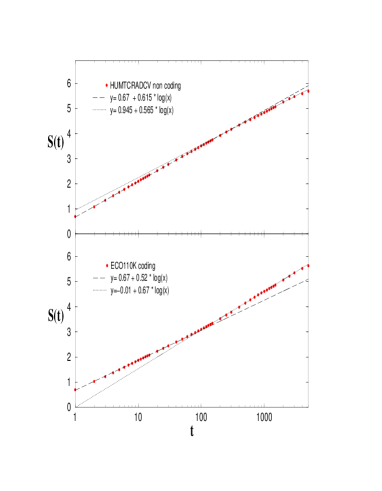
FIG. 1.: The diffusion entropy analysis for the two DNA sequences results in a scaling changing with time. For the HUMTCRADCV, the non-coding cromosomal fragment, the slope of the straight line is $\delta=0.615$ at short-time regime, and $\delta=0.565$ at long-time regime. For ECO110K, the coding genomic fragment, slopes are $\delta=0.52$ at short-time regime and $\delta=0.67$ at long-time regime

In Fig. 1b we consider the more delicate problem of a coding sequence: for ECO110K we observe at short time a slope $\delta=0.52$, very close to that of ordinary random walk, and at long-time a correlated diffusion with $\delta=0.67$, corresponding to $\mu=2.5$. We note that the authors of Ref. [13] using the DFA find in the short-time regime an uncorrelated diffusion with $\delta_{V}=0.51$ in agreement with the DE, and in the long-time regime a scaling $\delta_{V}=0.75$, which apparently conflicts with the finding of the DE method, yielding $\delta=0.67$. Note that the symbol $\delta_{V}$, with $V$ standing for variance, refers to the scaling detected by means of the DFA, which is in fact based on the variance measurement. Actually, we can prove that this apparent conflict yields a strong support to the main finding of our paper, that the DE method reveals the long-range correlations and the true asymptotic scaling of both coding and non-coding sequences.

In order to do so, we model a DNA sequence by adopting the Copying Mistaken Map (CMM) of Ref. [9]. As pointed out more recently [11], this model is equivalent to the Generalized Lévy Walk (GLW) [6]. The GLW, in turn, fits very well the observation made by the authors of Ref. [13] that the transition to super-diffusion in the long-time region is a manifestation of random walk patches with bias. The CMM corresponds to a picture where Nature builds up the real DNA sequence, either coding or non-coding, by using two different sequences. The former is a Random Sequence (RS) equivalent to assigning to any site the value +1 or -1 with equal probability. The latter sequence, on the contrary, is highly correlated and is obtained as follows. First of all, a sequence of integer numbers $l>0$ is drawn, with the inverse power law distribution:

$$p(l)=\frac{C}{(T+l)^{\mu}},~{}~{}2<\mu<3~{}.$$ (13)

Any drawing corresponds to fixing the length of a sequence of patches. To any patch is then assigned a sign, either +1 or -1, by tossing a coin. This prescription is virtually the same as that adopted to build up the symbolic sequence of Ref. [22], and corresponds to the intermittent condition of the Manneville map [23]. We call this correlated sequence Intermittent Randomness Sequence (IRS). As shown in refs. [12, 21], the diffusion process generated by the IRS is a Lévy diffusion. According to the CMM, Nature builds up the real DNA sequence by adopting for any site of the real sequence the nucleotide occupying the same site in the RS, with probability $p_{R}$, or the corresponding one of the IRS with probability $p_{L}=1-p_{R}$. The same prescription is used for modeling both the coding and non-coding DNA sequences, the only difference being in $p_{R}$, i.e. in the percentage of correlated to uncorrelated component: in particular the condition $p_{R}\gg p_{L}$ is valid for the coding DNA. The Lévy diffusion is faster than ordinary diffusion, and therefore is expected to become predominant, and so ostensible at long times, even when $p_{R}\gg p_{L}$. Of course, upon increase of $p_{R}$ Lévy statistics become ostensible at longer and longer times. As shown in Fig.2, the DE of HUMTCRADCV and ECO110K is perfectly reproduced by a CMM with $\mu=2.77$ and $\mu=2.5$, respectively. For the coding sequence $p_{R}=0.943$, i.e. the random component is predominant, while for the non-coding sequence $p_{R}=0.560$. It is worth to notice that with such values of $p_{R}$ the CMM also accounts for the correct slope of $S(t)$ vs. $ln(t)$ in the short-time regime.

Finally, we want to illustrate an important property of the DE method. The DE detects the real scaling of the distribution $\delta$, rather than the second moment scaling $\delta_{V}$. The two scaling values are identical only in the Gaussian case. In the Lévy case they are related [12] the one to the other by:

$$\delta=\frac{1}{3-2\delta_{V}}$$ (14)

We see that in the case of the non-coding sequence the DE yields an asymptotic scaling which is slightly smaller than the short-time scaling. This corresponds to the transition from the short-time Gaussian condition to the long-time Lévy condition, namely, to the transition from $\delta=\delta_{V}=0.61$ at short time to the value $\delta=1/(\mu-1)=0.565$ of the Lévy regime, with delta related now to $\delta_{V}=0.61$ by Eq. (14). In the coding case we see that the scaling detected by the DE method is $\delta=0.67$ that again is related to $\delta_{V}=0.75$ through Eq. (14).

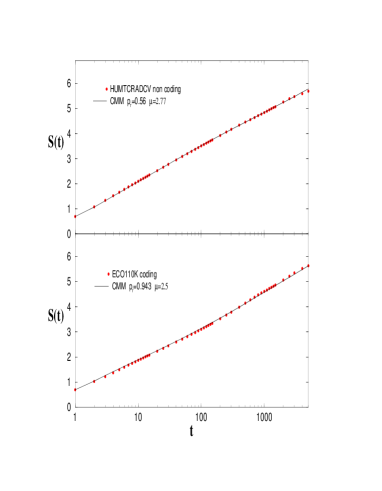
FIG. 2.: CMM simulation of the two DNA sequences. Fig. 2a shows the comparison between the DE analysis of HUMTCRADCV and an artificial sequence corresponding to the CMM model with $p_{R}=0.56$, $T=0.43$, $\mu=2.77$. Fig. 2b shows the comparison between the DE analysis of ECO110K and an artificial sequence corresponding to the CMM model with $p_{R}=0.943$, $T=45$, $\mu=2.5$.

In conclusion, this paper affords two important results. It proves that the DE method is a very reliable technique that detects the real scaling, and the real scaling does not coincide in general with that given by the DFA. The second result is that the joint use of the DE and DFA makes it possible to prove that the CMM, or the GLW, which is totally equivalent to the CMM [11], accounts for both coding and non-coding sequences. All this strengthens the idea that both non-coding and coding DNA sequences yield in the long-time limit an evident manifestation of long-range correlations, and confirms the claims of Ref. [11], where the non-Gaussian nature of the long-time regime was interpreted as a sign of the Lévy character of this region. The Lévy nature of the long-time statistics is now made compelling by the use of the DE, a method of statistical analysis so accurate as to perceive the difference between Lévy and Gauss scaling.

REFERENCES

- [1] National Center for Biotechnology Information. http://www.ncbi.nlm.nih.gov/
- [2] A. Torcini, R. Livi, A. Politi, A dynamical approach to protein folding, cond-mat/0103270.
- [3] C.-K. Peng, S.V. Buldyrev, A.L. Goldberger, S. Havlin, F. Sciortino, M. Simons and H.E. Stanley, Nature 356, 168 (1992).
- [4] W. Li, Int. J. Bifurcation Chaos Appl. Sci. Eng. 2, 137 (1992); W. Li and K. Kaneko, Europhys. Lett. 17, 655 (1992); W.Li, T. Marr, and K. Kaneko, Physica (Amsterdam) D 75, 392 (1994).
- [5] R. Voss, Phys. Rev. Lett. 68, 3805 (1992).
- [6] S.V. Buldyrev, A.L. Goldberger, S. Havlin, C.-K. Peng, M. Simons, and H.E. Stanley, Phys. Rev. E 47, 4514 (1993).
- [7] A.K. Mohanti and A.V.S.S. Narayana Rao, Phys. Rev. Lett. 84, 1832 (2000).
- [8] B. Audit, C. Thermes, C. Vaillant, Y. d’Aubenton-Carafa, J.F. Muzy, and A. Arneodo, Phys. Rev. Lett. 86, 2471 (2001).
- [9] P. Allegrini, M. Barbi, P. Grigolini and B.J. West, Phys. Rev. E 52, 5281 (1995).
- [10] P. Allegrini, M. Buiatti, P. Grigolini and B.J. West, Phys. Rev. E 57, 4588 (1998).
- [11] P. Allegrini, M. Buiatti, P. Grigolini and B.J. West, Phys. Rev. E 58, 3640 (1998).
- [12] P. Allegrini, P. Grigolini, B.J. West, Phys. Rev. E 54, 4760 (1996).
- [13] C. -K. Peng, S.V. Buldyrev, S. Havlin, M. Simons, H.E. Stanley and A.L. Goldberger. Phys. Rev. E 49, 1685 (1994).
- [14] B. B. Mandelbrot, Fractal Geometry of Nature, W.H. Freeman Co., New York (1988).
- [15] J. Feders, Fractals, Plenum Publishers, New York (1988).
- [16] N. Scafetta, P. Hamilton, P. Grigolini, in press on Fractals, cond-mat/0009020.
- [17] N. Scafetta, V. Latora, P. Grigolini, in preparation.
- [18] C. Beck, F. Schlögl, Thermodynamics of Chaotic Systems, Cambridge University Press, Cambridge (1993).
- [19] J. R. Dorfman, An Introduction to chaos in Nonequilibrium Statistical Mechanics, Cambridge University Press, Cambridge (1999).
- [20] V. Latora and M. Baranger, Phys. Rev. Lett. 82, 520 (1999).
- [21] M. Annunziato, P. Grigolini, Phys. Lett. A 269, 31 (2000).
- [22] M. Buiatti, P. Grigolini, L. Palatella, Physica A 268, 214 (1999).
- [23] P. Gaspard, X.J. Wang, Proc. Natl. Acad. Sci. USA 85, 4591 (1988).