Dynamics of on-line Hebbian learning with structurally unrealizable restricted training sets

Abstract

We present an exact solution for the dynamics of on-line Hebbian learning in neural networks, with restricted and unrealizable training sets. In contrast to other studies on learning with restricted training sets, unrealizability is here caused by structural mismatch, rather than data noise: the teacher machine is a perceptron with a reversed wedge-type transfer function, while the student machine is a perceptron with a sigmoidal transfer function. We calculate the glassy dynamics of the macroscopic performance measures, training error and generalization error, and the (non-Gaussian) student field distribution. Our results, which find excellent confirmation in numerical simulations, provide a new benchmark test for general formalisms with which to study unrealizable learning processes with restricted training sets.

On-line learning processes in artificial neural networks have been studied using statistical mechanical techniques for about a decade now (see e.g. [1, 2] for reviews). Initially, most dynamical studies were restricted to the regime where the number of training examples is larger than the number of learning steps, since this generally leads to Gaussian field distributions and relatively simple non-glassy dynamics. In practical situations, however, it is usually difficult to acquire large training sets, and one is therefore often forced to recycle the data in the training set. The latter situation, characterized by the presence of disorder (the composition of the training set) and non-trivial dynamics, was studied in e.g. [3, 4] (for binary weights), and in [5, 6, 7, 8, 9, 10] (for continuous weights). These studies generally involve approximations at some stage. This motivated [11], where it was shown how for the special case of on-line Hebbian learning the dynamics can be solved exactly (for restricted training sets), providing an excellent benchmark for general theories and approximation schemes. Some of the studies mentioned above involved learning from restricted but unrealizable training sets, where it is impossible for the student to achieve perfect performance, even if an infinitely large training set had been available. This could result from corruption by noise of realizable data (as in e.g. [8, 11]), or from structural mismatch between teacher and student. A typical toy model to realize the latter situation is obtained by using a perceptron with a reversed wedge transfer function as a teacher machine to train an ordinary perceptron [12, 13, 14] (note: there is also a relation between simple perceptrons with reversed wedge transfer functions and the so-called parity machines). Since all dynamical studies with restricted but unrealizable training sets have so far been carried out only for the data noise scenario, it would be of considerable interest to investigate exactly solvable models with restricted training sets but unrealizability due to structural mismatch. In this letter, we carry out such a study: we solve the dynamics of on-line Hebbian learning from unrealizable restricted training sets, for a teacher-student scenario where teacher and student have different transfer functions (a reverse-wedge and a sigmoidal one, respectively).

We investigate on-line learning in a ordinary student perceptron $S$ (whose weight vector is denoted by $J$), which tries to learn a task defined by a teacher perceptron $T_{a}$ (whose weight vector is denoted by $B$). The teacher is equipped with a reversed wedge transfer function, i.e. $T_{a}(y)={\rm sgn}[y(a-y)(a+y)]$ where $y=\mbox{\boldmath$B$}\,\cdot\,\mbox{\boldmath$\xi$}$ and $\mbox{\boldmath$\xi$}\in\{-1,1\}^{N}$ is the input vector, whereas $S(x)={\rm sgn}[x]$ with $x=\mbox{\boldmath$J$}\,\cdot\,\mbox{\boldmath$\xi$}$. The teacher’s weight vector $B$ is normalized such that $\mbox{\boldmath$B$}^{2}=1$, with $B_{i}={\mathcal{O}}(N^{-1/2})$ for each $i$. It is clear that in the limits $a\to 0$ and $a\to\infty$ (where $a$ characterizes the width of the reverse wedge) the task becomes realizable for the student, since $T_{0}(y)={\rm sgn}[-y]$ and $T_{\infty}(y)={\rm sgn}[y]$.

We define the conventional order parameters $Q[{\mbox{\boldmath$J$}}]\,\equiv\,\mbox{\boldmath$J$}^{2}$ and $R[{\mbox{\boldmath$J$}}]\,\equiv\,\mbox{\boldmath$B$}\cdot\mbox{\boldmath$J$}$. One of the main quantities of interest is the generalization error $E_{g}$, the probability of disagreement between teacher and student for input vectors taken randomly from the full set of all possible inputs:

$$E_{g}\equiv\langle{\Theta}[-T_{a}(y)S(x)]\rangle_{\mbox{\boldmath$\xi$}}=\int_{0}^{a}\!Du~{}{\rm erf}[r^{+}(u)]+\int_{a}^{\infty}\!Du~{}{\rm erf}[r^{-}(u)],$$ (1)

where $r^{\pm}(u)\,\equiv\,\pm Ru/\sqrt{2(Q\!-\!R^{2})}$, $Du\,\equiv(2\pi)^{-\frac{1}{2}}du~{}{\rm e}^{-u^{2}/2}$, $\Theta[\cdots]$ is the step function, and $\langle\cdots\rangle_{\mbox{\boldmath$\xi$}}$ denotes averaging over all $\mbox{\boldmath$\xi$}\in\{-1,1\}^{N}$. It was shown in [13] that the optimal normalized overlap $r=R/\sqrt{Q}$ (giving the smallest value of the generalization error) equals $1$ as long as the reversed wedge parameter $a$ is greater than $a=a_{\rm c1}=0.8$; $r$ suddenly changes from $1$ to $r_{*}=-\sqrt{(2\log 2-a^{2})/2\log 2}$ at $a=a_{\rm c1}$.

For this model system, we use the following on-line Hebbian learning rule

$$\mbox{\boldmath$J$}(\ell+1)=\left(1-\frac{\gamma}{N}\right)\mbox{\boldmath$J$}(\ell)+\frac{\eta}{N}T_{a}^{\mu(\ell)}\mbox{\boldmath$\xi$}^{\mu(\ell)}$$ (2)

where $\ell$ indicates the learning step, and $\eta$ and $\gamma$ represent the learning rate and the weight decay, respectively. The student learns from data picked randomly from the restricted training set $D=\{(\mbox{\boldmath$\xi$}^{\mu},T_{a}^{\mu}),~{}\mu=1,\ldots,p=N\alpha\}$.

To calculate macroscopic physical observables, averaged over the disorder (the composition of the training set) at any time, we need to distinguish between two averaging procedures [11]. The first is the average over all possible ‘paths’ ${\Omega}=\{\mu(0),\mu(1),\cdots,\mu(\ell),\cdots\}$ defining the actual sampling order from the training set:

$$\langle f(\mbox{\boldmath$\xi$}^{\mu(l)},T_{a})\rangle_{\Omega} \equiv \frac{1}{p}\sum_{\mu=1}^{p}f(\mbox{\boldmath$\xi$}^{\mu},T_{a})$$ (3)

The second is averaging over all training sets:

$$\langle f[(\mbox{\boldmath$\xi$}^{1},T_{a}^{1}),{\cdots},(\mbox{\boldmath$\xi$}^{p},T_{a}^{p})]\rangle_{\rm sets} \equiv 2^{-pN}\sum_{\mbox{\boldmath$\xi$}^{1}}{\cdots}\sum_{\mbox{\boldmath$\xi$}^{p}}\sum_{T_{a}^{1},{\cdots},T_{a}^{p}}\prod_{\mu}P(T_{a}^{\mu}|\mbox{\boldmath$\xi$}^{\mu})$$ (4)

$$\times~{}f[(\mbox{\boldmath$\xi$}^{1},T_{a}^{1}),\cdots,(\mbox{\boldmath$\xi$}^{p},T_{a}^{p})]$$

The key to the full solvability of the present model, as in [11], is the fact that (2) allows us to write $\mbox{\boldmath$J$}(m)$ (the student’s weight vector at $m$-th step) in explicit form as

$$\mbox{\boldmath$J$}(m)=\sigma^{m}\mbox{\boldmath$J$}(0)+\frac{\eta}{N}\sum_{\ell=0}^{m-1}\sigma^{m-\ell-1}T_{a}^{\mu(\ell)}\mbox{\boldmath$\xi$}^{\mu(\ell)}$$ (5)

where $\sigma\equiv(1-\eta/N)$. The above averaging procedures can now be carried out exactly.

In order to evaluate the training time dependence of the generalization error (1), following [11], we first calculate the following two macroscopic observables

$$Q(t)\equiv\displaystyle{\lim_{N{\rightarrow}\infty}}\langle\langle Q[{\mbox{\boldmath$J$}}(m)]\rangle_{\Omega}\rangle_{\rm sets},~{}~{}~{}~{}~{}~{}~{}~{}~{}R(t)\equiv\displaystyle{\lim_{N{\rightarrow}\infty}}\langle\langle R[{\mbox{\boldmath$J$}}(m)]\rangle_{\Omega}\rangle_{\rm sets},$$ (6)

where $t\equiv m/N$. Squaring (5) gives

$$\langle\langle Q[{\mbox{\boldmath$J$}}(m)]\rangle_{\Omega}\rangle_{\rm sets} = {\sigma}^{2Nt}Q_{0}+\frac{2\eta}{N}\sum_{\ell=0}^{m-1}{\sigma}^{2m-\ell-1}\langle\langle\mbox{\boldmath$J$}_{0}\cdot\mbox{\boldmath$\xi$}^{\mu(\ell)}T_{a}^{\mu(\ell)}\rangle_{\Omega}\rangle_{\rm sets}$$

$$+ \frac{\eta^{2}}{N^{2}}\sum_{\ell,\ell^{\prime}=0}^{m-1}\langle\langle{\sigma}^{m-\ell-1}{\sigma}^{m-\ell^{\prime}-1}\mbox{\boldmath$\xi$}^{\mu(\ell)}\cdot\mbox{\boldmath$\xi$}^{\mu(\ell^{\prime})}T_{a}^{\mu(\ell)}T_{a}^{\mu(\ell^{\prime})}\rangle_{\Omega}\rangle_{\rm sets}.$$

After calculating the averages $\langle\cdots\rangle_{\Omega}$ and $\langle\cdots\rangle_{\rm sets}$, and taking $N\to\infty$, we then obtain

$$Q(t) = {\rm e}^{-2\gamma t}Q_{0}+\frac{2\eta{\rho}_{a}R_{0}}{\gamma}{\rm e}^{-\gamma t}(1-{\rm e}^{-\gamma t})+\frac{\eta^{2}}{2\gamma}(1-{\rm e}^{-2\gamma t})$$ (7)

$$+\frac{\eta^{2}}{\gamma^{2}}(1/\alpha+{\rho}_{a}^{2})(1-{\rm e}^{-\gamma t})^{2}$$

where we defined $\rho_{a}\equiv\langle(\mbox{\boldmath$v$}\cdot\mbox{\boldmath$\xi$})T_{a}(\mbox{\boldmath$B$}\cdot\mbox{\boldmath$\xi$})\rangle_{\mbox{\boldmath$\xi$}}=\sqrt{2/\pi}(1\!-\!2\,{\rm e}^{-a^{2}/2})$. The quantity $\rho_{a}$ represents a kind of effective noise induced by the reversed wedge of the teacher. In a similar manner we obtain an exact expression for the student-teacher overlap $R(t)$:

$$R(t)={\rm e}^{-\gamma t}R_{0}+\frac{\eta\rho_{a}}{\gamma}(1-{\rm e}^{-\gamma t}).$$ (8)

The length of the component of $J$ which is orthogonal to $B$, $\sqrt{Q-R^{2}}$, is seen to remain independent of $\rho_{a}$. This is easily understood. The components of the input vectors which are orthogonal to $B$ are uncorrelated with the training outputs, so their evolution is not modified by the effect of the reversed wedge. From (7,8), in turn, we immediately obtain the generalization error at any time, via (1). For $t\to\infty$ this becomes

$${\lim_{t\rightarrow\infty}}E_{g}=\int_{0}^{a}\!Du~{}{\rm erf}[r_{*}^{+}(u)]+\int_{a}^{\infty}\!Du~{}{\rm erf}[r_{*}^{-}(u)]$$ (9)

with $r_{*}^{\pm}(u)\equiv\pm\rho_{a}u/\sqrt{\gamma+2/\alpha}$. In Figure 1, we show the asymptotic value of $E_{g}$ for $\alpha\rightarrow\infty$ (where we recover the unrestricted training sets behaviour), for different $\gamma$. We see that for $\gamma=0$, $E_{g}$ converges to $2\,{\rm erf}(a/\sqrt{2})$ for $a<a_{\rm c2}=\sqrt{2\log 2}$ and to $1-2\,{\rm erf}(a/\sqrt{2})$ for $a>a_{\rm c2}$, with an asymptotic scaling form $E_{g}\sim\alpha^{-1/2}$ as $\alpha\to\infty$ [13]. On the other hand, for $\gamma>0$, $E_{g}$ converges to $E_{g}^{*}|_{\alpha=\infty}$ as $E_{g}\sim\alpha^{-1}$.

Figure 1: Left: The asymptotic generalization error as a function of the width of the reversed wedge $a$ in the limit of $\alpha\rightarrow\infty$, for $\gamma=0$ (——), $\gamma=0.5$ (${\mathinner{\cdotp\cdotp\cdotp\cdotp\cdotp\cdotp}}$) and $\gamma=1$ (-  -  -  -). We chose $\eta=1$. Right: The corresponding normalized overlap $r=R/\sqrt{Q}$ which gives the generalization error in the left figure. The best possible values for the generalization error and the optimal normalized overlap are shown by thick lines.

For $\gamma=0$ and $a<a_{\rm c2}$, the asymptotic generalization error $E_{g}$ is seen to be larger than that corresponding to random guessing (over-training) [13]. When we introduce weight decay this phenomenon disappears. An optimal weight decay, minimizing the asymptotic $E_{g}$, exists for $a<a_{\rm c2}$ and is given by $\gamma_{\rm opt}=2a^{2}\rho_{a}^{2}/(2\log 2-a^{2})$.

For finite $\alpha$ and short times, $t\ll 1/\gamma$, we can expand (7) and (8) with respect to $\gamma t$ and find $R(t)=R_{0}+\eta\rho_{a}t,~{}Q(t)-R^{2}(t)=Q_{0}-R_{0}^{2}+\eta^{2}t+\eta^{2}t^{2}/\alpha$. In this regime the training time is too short for weight decay to have an effect. For $t\gg 1/\gamma$, on the other hand, it is clear from (7) and (8) that the order parameters $Q,R$ decay to their asymptotic values exponentially. For the case of $\gamma\rightarrow 0$, the small $\gamma t$ expansions are valid for all time. Upon expanding $E_{g}$ with respect to $\gamma$ we obtain

$$E_{g}\simeq\int_{0}^{a}\!Dx~{}{\rm erf}\left[\sqrt{\frac{\alpha}{2}}\rho_{a}x\right]+\int_{a}^{\infty}\!Dx~{}{\rm erf}\left[-\sqrt{\frac{\alpha}{2}}\rho_{a}x\right]+\frac{\alpha}{2t\sqrt{2\pi(1+\alpha\rho_{a}^{2})}}$$

We next turn to the student field distribution $P_{t}(x)$. If the number of examples in the training set is much larger than the number of training steps (i.e. for $\alpha\to\infty$), the student fields $x=\mbox{\boldmath$J$}\cdot\mbox{\boldmath$\xi$}$ are described by a Gaussian distribution, due to the central limit theorem. For $\alpha<\infty$ however, where the training sets are restricted and questions are recycled during the training process, complicated correlations build up and the field distribution generally acquires a non-Gaussian shape. In order to determine $P_{t}(x)$, we first calculate the joint distribution for student fields, teacher fields, and outputs (with $x,y\in\Re$ and $T_{a}\in\{-1,1\}$):

$$P(x,y,T_{a})=\lim_{N\to\infty}\frac{1}{p}\sum_{\mu=1}^{p}\langle\langle~{}\delta(x-\mbox{\boldmath$J$}\cdot\mbox{\boldmath$\xi$}^{\mu})\delta(y-\mbox{\boldmath$B$}\cdot\mbox{\boldmath$\xi$}^{\mu})\,\delta_{T_{a},T_{a}^{\mu}}~{}\rangle_{\Omega}\rangle_{\rm sets},$$

Its characteristic function is

$$\hat{P}_{t}(\hat{x},\hat{y},\hat{T})=\langle{\rm e}^{-i(\hat{x}x+\hat{y}y+\hat{T}T)}\rangle_{P_{t}(.,.,.)}$$

where $\langle f(x,y,T_{a})\rangle_{P_{t}(.,.,.)}=\int\!dxdy\sum_{T_{a}=\pm 1}P_{t}(x,y,T_{a})f(x,y,T_{a})$. Working out the (3,4) averages we obtain

$$\hat{P}_{t}(\hat{x},\hat{y},\hat{T}) = \displaystyle{\lim_{N\rightarrow\infty}}{\biggr{\langle}}\frac{1}{p}\sum_{\mu=0}^{p}{\exp}[-i\hat{x}\sigma^{Nt}\mbox{\boldmath$J$}_{0}\cdot\mbox{\boldmath$\xi$}^{\mu}-i\hat{y}\mbox{\boldmath$B$}\cdot\mbox{\boldmath$\xi$}^{\mu}-i\hat{T}T_{a}^{\mu}]$$

$$\times{\biggr{\langle}}{\exp}\left(-\frac{i\eta\hat{x}}{N}\sum_{\ell=0}^{Nt}\sigma^{Nt-\ell}\mbox{\boldmath$\xi$}^{\mu}\cdot\mbox{\boldmath$\xi$}^{\mu(\ell)}T_{a}^{\mu(\ell)}\right){\biggr{\rangle}}_{\Omega}{\biggr{\rangle}}_{\rm sets}.$$

By using the general relation

$$\hat{P}_{t}(\hat{x},\hat{y},\hat{T})=\int\!dxdy\sum_{T_{a}=\pm 1}e^{-i(\hat{x}x+\hat{y}y+\hat{T}T_{a})}P_{t}(x|y,T_{a})P(y,T_{a})$$ (10)

and some further algebra, following closely the procedure outlined in [11] (to which we refer for details), we then obtain the probability density $P_{t}(x)$ as

$$P_{t}(x) = \int\!Dy\sum_{T_{a}=\pm 1}P_{t}(x|y,T_{a})P(T_{a}|y)$$ (11)

$$= \int\!\frac{d\hat{x}}{2\pi}{\rm e}^{-\frac{Q}{2}x^{2}+{\chi}_{\rm r}(\hat{x})}\cos(\hat{x}x)\left[{\cos}(\chi_{\rm i}(\hat{x}))+G(\hat{x}R){\sin}(\chi_{\rm i}(\hat{x}))\right]$$

$$- 4{\rm e}^{-\frac{a^{2}}{2}}\!\int\!\frac{d\hat{x}}{2\pi}{\rm e}^{-\frac{Q}{2}\hat{x}^{2}+{\chi}_{\rm r}(\hat{x})}\cos(\hat{x}x)\sin(\chi_{\rm i}(\hat{x}))\int_{0}^{x\hat{R}}\!\!\!\frac{d\lambda}{\sqrt{2\pi}}{\rm e}^{\frac{\lambda^{2}}{2}}\cos(a\lambda)$$

where we defined the functions $\chi_{\rm r}$, $\chi_{\rm i}$ and $G$ as

$$\chi_{\rm r}(\hat{x})\equiv\frac{1}{\alpha}\int_{0}^{t}\!ds\left\{\cos\,[\eta\hat{x}{\rm e}^{-\gamma(t-s)}]-1\right\},~{}~{}~{}~{}\chi_{\rm i}(\hat{x})\equiv-\frac{1}{\alpha}\int_{0}^{t}\!ds\sin\,[\eta\hat{x}{\rm e}^{-\gamma(t-s)}]$$

$$G(\Lambda)\equiv{\rm e}^{\frac{1}{2}\Lambda^{2}}\int\!Dz~{}\sin(\Lambda|z|)=2\int_{0}^{\Lambda}\!\frac{d\lambda}{\sqrt{2\pi}}{\rm e}^{\frac{\lambda^{2}}{2}}.$$

Figure 2: The student field distribution $P_{t}(x)$ generated during on-line Hebbian learning, from a teacher with a reversed wedge of width $a=1$ and for $\eta=1$, $\alpha=0.5$ and $\gamma=0.5$, at times $t\in\{1,2,3,4\}$. Solid lines: the theoretical result (11). Histograms: results obtained via computer simulations for systems of size $N=10000$.

It follows from (11) that $P_{t}(x)$ is a symmetric function of $x$, for all times and all values of the reversed wedge width $a$. In the special cases $a=\infty$ and $a=0$ (where the task becomes realizable) we find our result (11) reducing to that of [11]:

$$P_{t}(x)=\int\frac{d\hat{x}}{2\pi}{\rm e}^{-\frac{1}{2}Q\hat{x}^{2}+\chi_{\rm r}(\hat{x})}\cos(\hat{x}x)\left\{{\cos}(\chi_{i}(\hat{x}))+(1\!-2\lambda)G(\hat{x}R)\sin(\chi_{\rm i}(\hat{x}))\right\}$$

with $\lambda=0$ for $a=\infty$, and $\lambda=1$ for $a=0$. This is consistent with [11], where the parameter $\lambda$ denoted the probability that a teacher output was corrupted by noise. Here we find that, if the width of the reversed wedge is zero, the transfer function of the teacher is the inverse of that of the student, and the the output of the teacher can be regarded as a noisy output with flip probability $\lambda=1$. In contrast, in the general case $0<a<\infty$, equation (11) shows that the effect of structural non-realizability can not be described by an ‘effective’ output noise. In Figure 2 we plot $P_{t}(x)$ as given by equation (11), for $a=1$, $\eta=1$ and $\gamma=0.5$, at different points in time, and we compare the result to the corresponding observations in numerical simulations (histograms). One clearly observes how $P_{t}(x)$ evolves from a Gaussian distribution at $t=0$ to a manifestly non-Gaussian one.

Finally, we calculate the training error $E_{t}$, which measures the average fraction of errors made by the student on inputs taken from the training set. It is given by

$$E_{t}=\int\!\!\!\int\!dxDy\sum_{T_{a}=\pm 1}{\Theta}[-T_{a}(y)S(x)]P_{t}(x|y,T_{a})P(T_{a}|y).$$

By using (10) and (11) we can obtain the explicit form of $E_{t}$ as

$$E_{t} = \frac{1}{2}-\int\!\frac{d\hat{x}}{2\pi\hat{x}}{\rm e}^{-\frac{Q}{2}\hat{x}^{2}+\chi_{\rm r}(\hat{x})}[G(\hat{x}R)\cos(\chi_{\rm i}(\hat{x}))-\sin(\chi_{\rm i}(\hat{x}))]$$ (12)

$$+4{\rm e}^{-\frac{a^{2}}{2}}\int\!\frac{d\hat{x}}{2\pi\hat{x}}{\rm e}^{-\frac{Q}{2}\hat{x}^{2}+\chi_{\rm r}(\hat{x})}{\cos}(\chi_{\rm i}(\hat{x}))\int_{0}^{\hat{x}R}\!\!\frac{d\lambda}{\sqrt{2\pi}}{\rm e}^{\frac{\lambda^{2}}{2}}\cos(a\lambda).$$

In Figure 3, we plot both the training error (12) and the generalization error (1) for four different values of the width $a$ of the teacher’s reversed wedge, viz. $a\in\{0.0,0.5,1.0,1.5\}$.

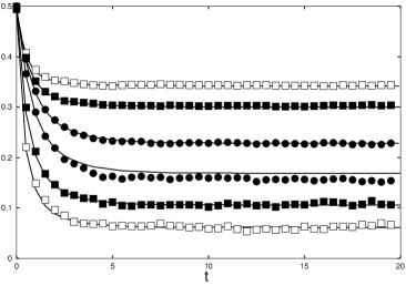
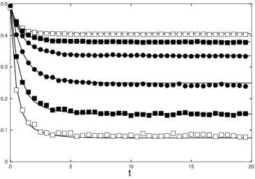
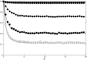
Figure 3: Training errors $E_{t}$ and generalization errors $E_{g}$ as functions of time, for different values of $\alpha$. In all cases $\eta=1$ and $\gamma=0.5$, with initial conditions $Q_{0}=1$ and $E_{g}(t=0)=0.5$. From the upper left panel to the lower right panel: $a=0.0,~{}0.5,~{}1.0$ and $1.5$. In each panel, the upper three solid lines indicate our theoretical results of $E_{g}$, together with the corresponding results of computer simulations: □($\alpha=0.5$), ■($\alpha=1.0$) and ●($\alpha=4.0$). The lower three lines are theoretical results for $E_{t}$, compared to the results of computer simulations, with □($\alpha=0.5$), ■($\alpha=1.0$) and ●($\alpha=4.0$). All simulations are carried out for systems of size $N=5000$.

In all case we find the theoretical results and the computer simulations to be in excellent agreement. In the limit $t\rightarrow\infty$ we also observe that the asymptotic values of both $E_{g}$ and $E_{t}$ indeed approach $E_{g}^{*}$ (see (9)) for increasing $\alpha$, as it should.

In conclusion, in this letter we have solved the dynamics of on-line Hebbian learning with structurally unrealizable restricted training sets exactly, for the case where a standard perceptron is being trained by a teacher perceptron with a reversed wedge transfer function. Although our solution applies only to Hebbian learning (as did the one in [11]), we believe that our results provide a valuable new benchmark against which to test (approximations made in) more general formalisms, such as generating functional analysis [3, 4, 10], dynamical replica theory [5, 6] or the cavity method [7].

The authors would like to thank King’s College London (JI) and the Tokyo Institute of Technology (ACCC) for their hospitality.

References

References

[1]
Opper M and Kinzel W 1995 in
Models of Neural Networks III,
eds. Domany E, van Hemmen J L and Schulten K (Berlin : Springer)
[2]
Mace C W H and Coolen A C C 1998 Statistics and Computing8 55
[3]
Horner H 1992 Z. Phys. B86 291
[4]
Horner H 1992 Z. Phys. B87 371
[5]
Coolen A C C and Saad D 1998 in
On-Line Learning in Neural Networks
ed. Saad D (Cambridge: U.P.) 303
[6]
Coolen A C C and Saad D 2000 Phys. Rev. E62 5444
[7]
Wong K Y M and Li S 2000 Phys. Rev. E62 4036
[8]
Coolen A C C and Mace C W H 2000 in Neural Information
Processing Systems 12 eds. Solla SA, Leen TK and Müller KR
(MIT Press) 237
[9]
Coolen A C C, Saad D and Xiong YS 2000 Europhys. Lett.51 691
[10]
Heimel J A F and Coolen A C C 2001 preprint cond-mat/0102272
[11]
Rae H C, Sollich P and Coolen A C C 1999
J. Phys. A: Math. Gen.32 3321
[12]
Watkin T L H and Rau A 1992 Phys. Rev.A45 4111
[13]
Inoue J, Nishimori H and Kabashima Y 1997 J. Phys. A: Math. Gen.30 1047
[14]
Kabashima Y and Inoue J 1998 J. Phys. A: Math. Gen.31 123