Curvature, hybridization, and STM images of carbon nanotubes

Abstract

The curvature effects in carbon nanotubes are studied analytically as a function of chirality. The $\pi$-orbitals are found to be significantly rehybridized in all tubes, so that they are never normal to the tubes’ surface. This results in a curvature induced gap in the electronic band-structure, which turns out to be larger than previous estimates. The tilting of the $\pi$-orbitals should be observable by atomic resolution scanning tunneling microscopy measurements.

The electronic band-structure of carbon nanotubes has been a topic of intense investigation ever since their discovery in 1991[1]. The basic electronic properties were quickly understood by numerical studies of the graphite tight binding band structure together with a simple zone folding model[2, 3]. In graphite the four outer electrons of carbon form three $sp^{2}$-hybridized $\sigma$-bonds and one $\pi$-orbital, which gives the conduction band with six Fermi points and a linear dispersion around each of them[4]. The electronic structure of the nanotube is then determined by the chiral wrapping vector along the direction $(n,m)$ since this determines whether the Fermi points satisfy the nanotube’s circumferential boundary conditions. In that model, tubes with a chiral vector that satisfies ${\rm mod}[(n-m)/3]=0$ have their Fermi point in the allowed $k$-space and thus are considered to be metallic, while all other tubes are semiconducting[2, 3]. But even the “metallic” tubes may open a small gap if the bond symmetry is broken due to curvature[5, 6], which has been analyzed in analytical studies in terms of a one-orbital tight binding approximation[7, 8].

One difficulty in predicting the effect of curvature on the electronic properties has been to determine the exact bond energies in the curved graphite sheet to arrive at an analytical formula. So far it has explicitly been assumed that the $\pi$-orbitals are orthogonal to the tubes surface[7], which is a common overly simplified picture that has also been used in a previous report by the authors[8]. We show in this Letter, however, that the $\pi$-orbitals are never orthogonal to the surface, and instead are rehybridized due to the effect of the lower lying $\sigma$-bonds. Typically such a mixing effect is always expected, but early studies have estimated that this band-mixing can be neglected[3]. However, for the case of metallic tubes we find that this mixing plays an important role, which is crucial in determining an analytic formula for the curvature induced bandgap as a function of chirality and curvature. Moreover, we can predict the explicit angles of the $\pi$-orbitals relative to the tubes surface, which should be observable in atomic resolution pictures from Scanning Tunneling Microscopy (STM) experiments.

Our starting point is the well-defined geometrical structure of the carbon nanotubes by describing it in terms of an “unrolled” graphite sheet. The $\sigma$-bonds lie along three vectors which can be expressed in a coordinate system of the circumferential and translational axes $(\hat{c},\hat{t})$ in terms of the chiral indices $(n,m)$.

$$\begin{array}[]{l}\vec{R}_{1}=\frac{a}{2c_{h}}[(n+m)\hat{c}+\frac{1}{\sqrt{3}}(n-m)\hat{t}]\\ \vec{R}_{2}=\frac{a}{2c_{h}}[-n\hat{c}+\frac{1}{\sqrt{3}}(n+2m)\hat{t}]\\ \vec{R}_{3}=\frac{a}{2c_{h}}[-m\hat{c}-\frac{1}{\sqrt{3}}(2n+m)\hat{t}],\end{array}$$ (1)

where $a\approx 2.49\rm\AA$ is the length of the honeycomb unit vector and $c_{h}=\sqrt{n^{2}+nm+m^{2}}$ is the circumference in units of $a$.

In the regular $sp^{2}$ hybridization of the unrolled graphite sheet the four atomic wave functions can be written as

$$|\sigma_{i}^{0}\rangle = \sqrt{\frac{1}{3}}|s\rangle+\sqrt{\frac{2}{3}}\left(\sin\beta_{i}|t\rangle+\cos\beta_{i}|c\rangle\right)~{}~{}~{}~{}~{}~{}~{}~{}~{}i=1,2,3$$ (2)

$$|\pi^{0}\rangle = |z\rangle$$ (3)

where $|s\rangle$ stands for the atomic s-orbital and $|t\rangle,|c\rangle,|z\rangle$ denote the p-orbitals along the translational, circumferential and normal directions in a nanotube, respectively. Here $\beta_{i}$ are the angles of the bonds relative to the circumferential direction ($\cos\beta_{i}\equiv\hat{c}\cdot\hat{R}_{i}$). Each carbon atom has its own local coordinate system, where the $z$-direction is given by the normal direction to the graphite surface. In a nanotube neighboring atoms have a relative angle $2\alpha_{i}$ between their $z$-directions as shown in Fig. 1 with

$$\sin\alpha_{i}=\frac{\hat{c}\cdot\vec{R}_{i}}{2r}=\frac{a}{2\sqrt{3}r}\cos\beta_{i},$$ (4)

where $r=ac_{h}/2\pi$ is the radius of the nanotube. We call this a geometrical tilting of the $\pi$-orbitals, which is known to induce a curvature gap[7, 8] and is predicted to cause a stretching around the circumference of STM images[9].

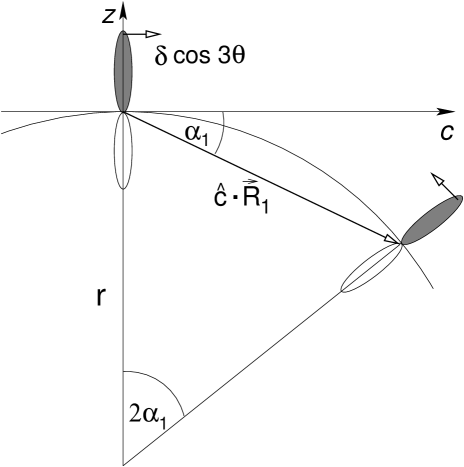
FIG. 1.: Schematic cross-section of a bond $\vec{R}_{1}$ in a nanotube with radius $r$. The $\pi$-orbitals are no longer normal to the tubes surface, but are titled by the hybridization angle $\delta=a/4\sqrt{3}r$ (small arrows).

However, in addition we find an equally important contribution to the tilting from hybridization, which we will discuss next. This hybridization comes from the fact that in a nanotube the three $\sigma$-bonds are not in the same plane, but instead directed towards the positions of the nearest neighboring carbon atoms, ie. they are tilted down by the angles $\alpha_{i}$ relative to the tangential $c$-direction as shown in Fig. 1. The hybridization of the $\sigma$-bonds is therefore changed from the uncurved expression for $|\sigma^{0}_{i}\rangle$ in Eq. (2) to

$$|\sigma_{i}\rangle=s_{i}|s\rangle$$ (5)

$$+ \sqrt{1-s_{i}^{2}}\left(\,\sin\beta_{i}|t\rangle+\cos\alpha_{i}\cos\beta_{i}|c\rangle-\sin\alpha_{i}\cos\beta_{i}|z\rangle\,\right),$$ (6)

where the mixing parameters $s_{i}$ (expanded around $s_{i}\approx\sqrt{1/3}$) can be determined by the three orthonormality conditions between the $\sigma$ bonds $\langle\sigma_{i}|\sigma_{j}\rangle=\delta_{ij}$. The hybridized $\pi$-orbital can now be calculated in terms of the local basis of atomic orbitals by using the orthonormality conditions

$$\langle\pi|\sigma_{i}\rangle=0.$$ (7)

In what follows we will only work to lowest order in the curvature parameter $a/r=2\pi/c_{h}$ because energy band repulsion will give higher order corrections for narrow nanotubes. In particular, it has been shown by ab initio LDA calculations that the $\sigma$-bands are pushed up above the Fermi points for very small radii $r\lesssim 2.4\rm\AA$[10]. The straightforward hybridization analysis here is therefore only correct as a lowest order approximation in $a/r\ll 1$, but gives a useful physical picture for most observed nanotubes.

From Eqs. (5) and (7) we can now find the correct expression for the $\pi$-orbitals to lowest order in $a/r$

$$|\pi\rangle\simeq|z\rangle+\frac{a}{4\sqrt{3}r}\left(\sqrt{2}|s\rangle\pm\sin 3\theta|t\rangle\pm\cos 3\theta|c\rangle\right),$$ (8)

where $\theta$ is the so-called chiral angle $\theta\equiv{\rm min}(|\beta_{1}|,|\beta_{2}|,|\beta_{3}|),\ 0\leq\theta\leq\pi/6$ as shown in Fig. 2. The different $\pm$ signs in Eq. (8) refer to neighboring atoms $A$ and $B$ in the bipartite graphite lattice, since their bonds and the corresponding angles $\beta_{i}$ point in opposite directions as indicated in Fig. 3.

FIG. 2.: The three $\sigma$-bonds around a carbon atom in the rolled up graphite lattice. The unhybridized $\pi$-orbital is marked by the black dot in the center as seen from above. The predicted hybridization in Eq. (8) of the $\pi$-orbital is indicated by the triple arrow with $\delta=a/4\sqrt{3}r$. The example shown here corresponds to a (9,3) nanotube seen from a height of $h\approx 3a$. Note, that the angle $\theta$ in Eq. (8) can in fact be chosen to be any of the three angles $\beta_{i}$ of the bond vectors relative to the $c$-direction to get the correct hybridization.

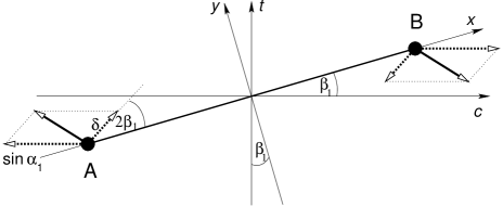
FIG. 3.: Two neighboring carbon atoms with with the predicted hybridization angle $\delta=a/4\sqrt{3}r$ and geometrical curvature effects $\sin\alpha_{i}=2\delta\cos\beta_{i}$, seen from above. The example shown corresponds to the bond $\vec{R}_{1}$ in a (9,3) nanotube.

The physical interpretation of Eq. (8) is very intuitive. The $\pi$-orbital is always inclined by the hybridization angle $\delta$ of size $\delta=a/4\sqrt{3}r$ relative to the normal direction to the tube’s surface. However, the direction of this inclination rotates with $3\theta$ relative to the $c$-direction as indicated in Fig. 2. It can be verified that the three angles between the $\pi$-orbital and each of the $\sigma$-bonds in Eq. (5) are equal as should be expected by symmetry. Sometimes it is useful to express the hybridization in Eq. (8) in terms of the chiral indices $(n,m)$ using

$$\sin 3\theta = (n-m)(2m^{2}+5mn+2n^{2})/2c_{h}^{3}$$ (9)

$$\cos 3\theta = 3\sqrt{3}mn(m+n)/2c_{h}^{3}$$ (10)

At this point we can proceed to calculate the hopping matrix elements $\gamma_{i}$ between neighboring $\pi$-orbitals which will determine the one-orbital tight binding band structure. Following the Slater-Koster scheme[12] for calculating the matrix elements $\gamma_{i}$ between tilted $\pi$-orbitals we need to use a common coordinate basis for the two neighboring atoms. Both the hybridization effect in Eq. (8) and the geometrical tilting with $\alpha_{i}$ in Eq. (4) can easily be expressed in the coordinate system where the bond vector $\vec{R}_{i}$ between two neighboring atoms $A$ and $B$ defines the x-direction as shown in Fig. 3

$$|\pi\rangle \simeq |z\rangle+\sqrt{2}\delta|s\rangle\pm\left(\delta\cos 2\beta_{i}-\sin\alpha_{i}\cos\beta_{i}\right)|x\rangle$$ (12)

$$\pm\left(\delta\sin 2\beta_{i}+\sin\alpha_{i}\sin\beta_{i}\right)|y\rangle,$$

where $\delta=a/4\sqrt{3}r$ and the angles $\beta_{i}$ are now defined in respect to the $A$ site. Using the notation in Ref. [6], we can use the overlap integrals between neighboring $s$- and $p$-orbitals $V_{ss\sigma},V_{sp\sigma},V_{pp\sigma},V_{pp\pi}$ to calculate the hoping matrix elements $\gamma_{i}$

$$\gamma_{i}=V_{pp\pi}$$ (13)

$$- \frac{a^{2}}{48r^{2}}\left([3+8\sin^{2}2\beta_{i}]V_{pp\pi}-2V_{ss\sigma}-2\sqrt{2}V_{sp\sigma}+V_{pp\sigma}\right).$$ (14)

Here we have also used the second order term for the $|z\rangle$ orbital, which contributes to this expression.

The most interesting aspect of the electronic structure in metallic tubes is the size of the gap due to curvature as a function of the chiral wrapping vector, which we can now calculate directly. After having determined the rehybridized orbitals and hoping integrals, we can typically ignore the lower lying bands in further calculations and use a simple one-orbital tight binding approximation. In this model the gap can be calculated from the positions of the Fermi points $\vec{k}_{F}$ in the curved graphite sheet which in turn are determined in terms of the new hopping matrix elements $\gamma_{i}$[4]

$$\sum_{i=1}^{3}\gamma_{i}e^{i\vec{k}_{F}\cdot\vec{R}_{i}}=0.$$ (15)

Using the linear dispersion relation and the position of the quantization lines it is then straightforward to derive the gap equation[8, 11] assuming that the tube is metallic ${\rm mod}[(n-m)/3]=0$

$$E_{g}=\frac{2\sqrt{3}}{a}\left|\sum_{i=1}^{3}\,(V_{pp\pi}-\gamma_{i})\,\vec{R}_{i}\cdot\hat{t}\right|=\frac{a^{2}}{4r^{2}}V_{pp\pi}\sin 3\theta.$$ (16)

This surprisingly simple formula reconfirms again the notion that armchair tubes $(n=m,\ \theta=0)$ do not have a gap from curvature, while zigzag-tubes $(m=0,\ \theta=\pi/6)$ and all other metallic tubes acquire a gap of order $1/r^{2}$[5]. For semiconducting tubes with an intrinsic gap of order $1/r$ this geometrical and hybridization correction to the gap can typically be neglected, but for metallic tubes it is essential to take the proper hybridization into account. While the dependence of the gap on the chiral angle agrees with previous analytic studies[7, 8], the expression in Eq. (15) is by a factor of four larger than those estimates, which have not considered hybridization effects.

We now discuss how the rehybridization may be observable in STM experiments. Already without rehybridization the directions of the $\pi$-orbitals in a curved geometry can affect the STM images as predicted in Ref. [9]. In that study only the geometrical effects were taken into account, which resulted in an effective stretching of the STM image along the circumference by the amount $x_{c}\to x_{c}(1+{h}/{r})$, where $h$ is the height of the STM tip relative to the nanotube surface. However, the tilting $\delta$ caused by hybridization is of similar size and will results in an additional distortion of the STM image in both transverse and circumferential directions, but alternating for the inequivalent $A$ and $B$ atoms

$$x_{c} \to x_{c}\left(1+\frac{h}{r}\right)\pm\frac{ha}{4\sqrt{3}r}\cos 3\theta$$ (17)

$$x_{t} \to x_{t}\pm\frac{ha}{4\sqrt{3}r}\sin 3\theta,$$ (18)

where $x_{c}$ and $x_{t}$ measure distances in the circumferential and transverse directions, respectively. Interestingly, the distortion from the hybridization depends again to linear order on $h/r$ in all tubes, as opposed to the curvature gap which is a correction of second order and only matters for metallic tubes. If we consider this distortion for the case of a zigzag tube with $\theta=\pi/6$, we see that the hexagons of the graphite sheet will appear compressed in the transverse direction, but stretched around the circumference as shown in Fig. 4. For the armchair tubes $\theta=0$ on the other hand there is no deformation along the transverse direction, but the hexagons are still deformed along the circumferential direction as shown in Fig. 4. To observe the hybridization effects it would therefore be most advantageous to scan along the ridge of a zigzag tube and average or Fourier transform the image over a distance of several hundred carbon sites, preferably for more than one value of the height $h$.

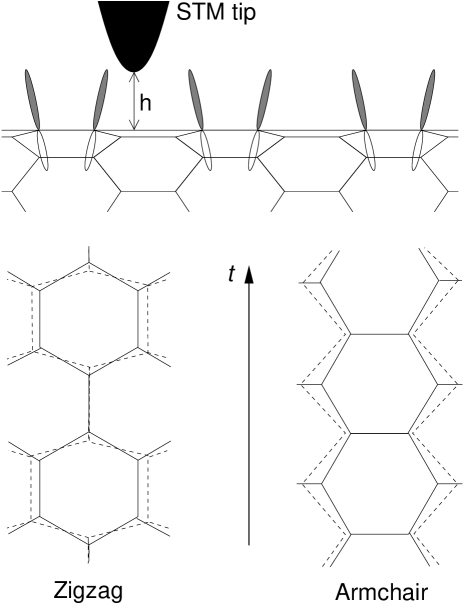
FIG. 4.: The predicted distortion of an STM image (dashed lines). For a zigzag tube we find a pronounced squaring of the hexagons and a change of the lattice constants along the transverse directions. For the armchair tube the image is only affected along the circumferential direction.

In summary we have shown that it can be expected that the curvature of carbon nanotubes will result in a significant rehybridization of the $\pi$-orbitals. This rehybridization will affect the energy gap and will also manifest itself in a well-defined distortion of atomic resolution STM images given by Eq. (17). To lowest order in the curvature parameter $a/r$ the hybridization angle was found to be $\delta=a/4\sqrt{3}r$, resulting in an energy gap which is significintly higher than previous analytical studies[7, 8] as well as numerical estimates[6]. It is not clear to us what assumptions were used to model the curvature in the tight binding calculations of Ref. [6], but the results coincide with analytic studies[7, 8] that did not take any hybridization into account. Higher order effects and energy band repulsion will modify the size of the hybridization angle $\delta$ and therefore also the energy gap. However, the direction of the hybridization given by $3\theta$ relative to the circumference is correct as can be seen by symmetry arguments. The exact size of the hybridization angle can most reliably be found by analyzing STM images as outlined above, which in turn would lead to a more reliable estimate of the curvature gap.

REFERENCES

- [1] S. Iijima, Nature, 354, 56 (1991)
- [2] N. Hamada, S. Sawada, and A. Oshiyama, Phys. Rev. Lett. 68, 1579 (1992).
- [3] R. Saito, M. Fujita, G. Dresselhaus, and M. S. Dresselhaus, Phys. Rev. B 46, 1804 (1992).
- [4] P.R. Wallace, Phys. Rev. 71, 622 (1947).
- [5] C. T. White, J. W. Mintmire, R. C. Mowrey, D. W. Brenner, D. H. Robertson, J. A. Harrison and B. I. Dunlap in Buckminsterfullerenes, Edited By W. Edward Billups and Marco A. Ciufolini, VCH publishers (1993).
- [6] J. W. Mintmire, D. H. Robertson and C. T. White, J. Phys. Chem. Solids 54, 1835 (1993); J. W. Mintmire and C. T. White, Carbon 33 893 (1995).
- [7] C. L. Kane and E. J. Mele, Phys. Rev. Lett. 78, 1932 (1997).
- [8] A. Kleiner and S. Eggert, Phys. Rev. B 63, 73408 (2001).
- [9] V. Meunier and Ph. Lambin, Phys. Rev. Lett. 81, 5588 (1998)
- [10] X. Blase et al. Phys. Rev. Lett. 72, 1878 (1994)
- [11] L. Yang and J. Han, Phys. Rev. Lett. 85, 154 (2000).
- [12] J. C. Slater and G. F. Koster, Phys. Rev. 94, 1498 (1954).