Out of equilibrium dynamics of a Quantum Heisenberg Spin Glass

Abstract

We study the out of equilibrium dynamics of the infinite range quantum Heisenberg spin glass model coupled to a thermal relaxation bath. The $SU(2)$ spin algebra is generalized to $SU(N)$ and we analyze the large-$N$ limit. The model displays a dynamical phase transition between a paramagnetic and a glassy phase. In the latter, the system remains out of equilibrium and displays an aging phenomenon, which we characterize using both analytical and numerical methods. In the aging regime, the quantum fluctuation-dissipation relation is violated and replaced at very long time by its classical generalization, as in models involving simple spin algebras studied previously. We also discuss the effect of a finite coupling to the relaxation baths and their possible forms. This work completes and justifies previous studies on this model using a static approach.

The study of the non-equilibrium dynamics of classical glassy systems has been the subject of an intense research in the last decade. A lot of progress has been made reviewDYN using scaling arguments, phenomenological approaches and mean field theory. One of the major achievement is the theoretical explanation of the aging phenomena, which is one of the most striking feature of glassy systems. The analysis of the out of equilibrium of (classical) mean field spin glasses has played a major role for several reasons. It has furnished a framework to understand, interpret and analyze the experimental results and it has given important predictions on the violation and the generalization of the fluctuation dissipation relation out of equilibrium CugliandoloKurchanPRL which has been experimentally tested recently FDTexp .

Usually, many glassy systems can be analyzed within a classical approach since they are characterized by transition temperatures at which quantum mechanical effects are not relevant. Nevertheless, there are also interesting cases in which the critical temperature can be lowered to zero tuning a parameter which controls the strength of quantum fluctuations. This give rise to a quantum critical point at zero temperature SachdevBook . Close to this point, the quantum fluctuations are very important and cannot be neglected. One example which has received much attention recently is the insulating magnetic compound ${\mbox{LiHo}_{x}\mbox{Y}_{1-x}\mbox{F}_{4}}$ which is an experimental realization of an Ising spin glass in a transverse field WuBitkoRosenbaumAeppli . Other systems where glassy properties in the presence of quantum fluctuations have been observed are mixed hydrogen bonded ferro-antiferro electric crystals FerroExp , interacting electron systems Zvi , cuprates like La_2-xSr_xCuO₄ ChouSG , amorphous insulators Osheroff1+Osheroff2+Osheroff3 .

The theoretical study of quantum glassy systems has been performed following two different and complementary routes. One dimensional models (like the Random Transverse Ising spin chain) has been extensively studied and it has been shown that the Griffiths-McCoy singularities are very important close to the quantum critical point PapierTheoGriff . On the other hand, after the work of Bray and Moore BrayMoore much attention has been focused on infinite dimensional (mean field) models ShuklaSingh ; YamamotoIshii ; DobroThiru ; MillerHuse ; kopec ; GiamarchiLedoussal ; GrempelRozenberg ; GrempelRozenberg2 ; SGletter ; SGlong ; Isya ; rsy ; Niri ; CugliandoloLozano ; CugliandoloPspinQLettre . In particular, recently, it has been shown CugliandoloGrempelDaSilva that for the quantum spherical p-spin glass model the quantum fluctuations drive the transition toward a first order quantum phase transition at low temperature. The same phenomenon has been observed experimentally for the insulating magnetic compound ${\mbox{LiHo}_{x}\mbox{Y}_{1-x}\mbox{F}_{4}}$ WuBitkoRosenbaumAeppli . In QuantumTAP it has been argued that this phenomenon is to be expected in a large class of systems.

In contrast, the study of real time out-of-equilibrium dynamics of quantum glassy system is a recent subject and only very few results are available at the time of this writing. In a first pioneering paper, Cugliandolo and Lozano CugliandoloLozano presented a detailed solution of a quantum version of the $p-$spin model. They showed how the out of equilibrium behavior of classical glassy systems is affected by quantum fluctuations. In particular they found that the low temperature glassy phase is characterized by the aging phenomenon. In this regime, the fluctuation dissipation relation is violated and it is generalized to a form that coincides with the (generalized) classical one. This could seem natural since at low frequency the quantum fluctuation relation coincides with its $\hbar\rightarrow 0$ limit (for a bosonic system). Indeed it has been shown in ChamonRotorsLettre ; ChamonRotors that for models with simple commutation relations (particles and rotors) the classical nature of the generalized fluctuation dissipation relation is due to the fact the dynamical equations are fixed point of the re-parameterization group of time transformations and the renormalized aging dynamics becomes classical at the fixed point. The quantum mechanics enters only as a renormalization of the coefficients of the dynamical equations.

However what happens for models with a non trivial spin algebras, as the $SU(N)$ model studied in SGlong ; SGletter remained an open question. The study of the out of equilibrium dynamics of this type of quantum glassy systems is the main aim of this paper. We will focus on the quantum Heisenberg Spin Glass where the $SU(2)$ spin symmetry group is replaced by $SU(N)$ and take the large $N$-limit. In this model, the spin are true quantum spins, i.e. with non trivial commutation relations, and this introduces in the problem Berry phases which play an important role SachdevBook . Recently a detailed mean field solution using an equilibrium approach has been presented in SGlong ; SGletter . The model displays a second order phase transition at a temperature $T_{eq}$ between a paramagnetic phase and a spin glass phase, and it is solved by a one-step replica symmetry breaking scheme. Moreover, using a procedure called “the marginality condition”, the existence of a dynamical transition has been predicted at a temperature $T_{d}>T_{eq}$. First introduced and discussed in the quantum case in GiamarchiLedoussal , this prescription was used in SGlong ; SGletter since it lead to the most acceptable solutions. Recently, the TAP approach has been fully generalized to quantum systems QuantumTAP . The relationship between TAP and replica approaches gives a further hint on why one has to choose the marginal solution in the replica method. In fact this solution is related to the marginally stable TAP states which have some flat directions around them in the (quantum) free energy landscape, on the contrary of all the others which are completely stable. Assuming that the quantum out of equilibrium dynamics is dominated by the presence of flat directions around the marginally stable TAP states, as it happens in the classical case, one finds a more natural justification of “the marginality condition”. However, only a complete dynamical analysis can fully justify this procedure. The analysis performed in this paper of the real time out of equilibrium dynamics, using the Schwinger-Keldysh close time formalism Keldysh ; RammerSmith , shows indeed its correctness.

This paper is organized as follows : in section I, we present the model and the relaxation bath coupled to it. In section II, we present the dynamical large-$N$ equations for the retarded and Keldysh correlation functions and we explain their derivation and how to deduce them from the simpler imaginary time equations. In section III, we present both an analytical and a numerical analysis of the dynamical equations. Numerical evidence for aging and for a generalized fluctuation-dissipation theorem in the aging regime are presented. Moreover the analysis of the aging regime justify the “marginality condition” used in previous works SGletter ; SGlong . Finally, in section IV, we briefly discuss the effect of a finite coupling to the relaxation bath.

I The Heisenberg spin glass and the relaxation bath

The model considered in this paper is a quantum Heisenberg spin-glass on a completely connected lattice of ${\cal N}$ sites with quenched disordered couplings $J_{ij}/\sqrt{{\cal N}N}$ which are independent random Gaussian variable of zero mean and a variance $\overline{J_{ij}^{2}}/({\cal N}N)=J^{2}_{H}/({\cal N}N)$. Each spin is linearly coupled to a thermal bath. Moreover we generalize the $SU(2)$ spin symmetry group to $SU(N)$ and we take the large $N$-limit. This generalization allows us to obtain a tractable model which has still highly non trivial quantum effects and reproduces qualitatively well the known results for the $SU(2)$ model, as far as it has been possible to compare the $N=2$ and the $N=\infty$ casesSGletter ; SGlong ; GrempelRozenberg . The Hamiltonian reads:

$$H=\frac{1}{\sqrt{{\cal N}N}}\sum_{i<j}J_{ij}\vec{S}_{i}\cdot\vec{S}_{j}+\frac{J_{B}}{N\sqrt{\gamma}}\sum_{i\alpha}\vec{S}_{i}\cdot\vec{s}_{i\alpha}+H_{{\text{Bath}}}(\vec{s})$$ (1)

where the scaling of the spin-spin couplings and the antiferromagnetic spin-bath coupling has been chosen in such a way to obtain a sensible large ${\cal N}$, $N$ limit, i.e. $J^{2}_{H},J_{B}\propto O(1)$. The first term is the Quantum Heisenberg spin glass Hamiltonian, the third and the second terms represent respectively the thermal bath of spins $\vec{s}_{i}$ and its coupling to the spins $\vec{S}_{i}$ via the coupling constant $J_{B}$. Let us now discuss them separately.

Among the possible representation of the $SU(N)$ spin, two versions have been studied SGletter ; SGlong : the bosonic model, in which the spin operator $S$ is represented using constrained Schwinger bosons $b$ by

$$S_{\alpha\beta} =b^{\dagger}_{\alpha}b_{\beta}-S\delta_{\alpha\beta}$$ (2a)

$$\sum_{\alpha=1}^{N}b^{\dagger}_{\alpha}b_{\alpha} =SN$$ (2b)

and the fermionic model, in which the spin operator $S$ is represented similarly using Abrikosov fermions $f$ by $S_{\alpha\beta}=f^{\dagger}_{\alpha}f_{\beta}-S\delta_{\alpha\beta}$, with the constraint $\sum_{\alpha}f^{\dagger}_{\alpha}f_{\alpha}=SN$ ($0\leq S\leq 1$). See AuerbachBook for an introduction to this two representations. The two models are technically very similar but there is an important physical difference between them : in the fermionic model, quantum fluctuations are so strong in the large-$N$ limit that the spin glass ordering is destroyed SachdevYe (the critical temperature vanishes when $N$ diverges SGlong ), whereas in the bosonic model, a spin glass phase exists at low temperature SGletter ; SGlong . In the following we will focus mainly on the latter one and we briefly discuss some results for the former one at the end of Section III. In the model we study, the size $S$ of the spin is a fixed, tunable parameter which controls the strength of quantum fluctuations (since $N=\infty$ it is moreover continuous). Let us emphasize that the $N\rightarrow\infty$ limit is not the classical limit : as shown in SGletter ; SGlong , the model is classical for large $S$ (but not a very low temperature), while it is “more quantum” (i.e. the quantum fluctuations are more important) at low $S$ and displays a quantum critical point at $S=0$ where the spin glass temperature vanishes.

Moreover, it is important to remark that the real physical object is the spin $S$, not to the boson $b$ or the fermion $f$ which should be considered here more as mathematical tools. Technically, this leads to a simple $U(1)$ gauge invariance of the bosonic or fermionic theory (we can always multiply the $b$ or the $f$ by a phase) whose consequences will be explained later.

Let us now discuss the role of the relaxation bath terms in (1). Its presence is necessary to allow the energy dissipation. It guarantees the relaxation toward equilibrium above the dynamical transition $T_{d}$ and it is required to obtain an aging regime below $T_{d}$. In this paper, we are mostly interested in the $J_{B}\rightarrow 0$ limit, which must always be taken after the long time limit : for example, the dependance of the equilibrium state in $J_{B}$ is expected to be smooth in this limit, although the transient time towards the equilibrium diverges. The bath we have considered in (1) is supposed, as usual, to be very big and always in equilibrium at a finite temperature $T=1/\beta$. For further simplification we take independent baths from site to site (labeled by $i$), and the spins $\vec{s}_{i}$ carry an additional degree of freedom $\alpha$, with $1\leq\alpha\leq N\gamma$ (where $\gamma$ is a constant), which ensures that the bath is much bigger than the spins it is coupled to. Moreover we will make the assumption of factorized initial condition QuantumBrownian . By this we mean that the initial density matrix is a product of an equilibrium density matrix for the bath and an initial density matrix for the system. Since $b$ (or $f$) is not the physical object, the bath should respect the $U(1)$ invariance, i.e. it must couple to two $b$’s and we do not consider baths coupling linearly to $b$ in this paper. Of course many different choices are possible. We first consider a “generic” bath $H_{bath}(\vec{s})$ of interacting spins $\vec{s}$ and expand the Keldysh effective action for $S$ at second order in the coupling constant $J_{B}$ (the first order vanishes). In the dynamics, the bath will then appear only through its susceptibility $\chi_{0}$ (see section II). This approach is appropriate when we only consider the bath as a device to provide thermalization. One could wonder how correct is to study a low temperature glassy phase using a perturbative treatment of the coupling to the environmental heat bath. In Section IV we will show that this is not a limitation and we will briefly discuss the simplest type of spin bath which will turns out to be a Kondo bath.

II The dynamical equations

In order to study the real time dynamics, we use the Keldysh method Keldysh : the time evolution operator is written as a path integral over 2 times $t_{+}$ and $t_{-}$, running from $0$ to infinity forward and backward respectively. In the classical limit, this method reduces to the Martin-Siggia-Rose-DeDominicis-Janssen formalism (See Appendix C of CugliandoloLozano ). We take an infinite temperature initial condition at $t=0$ and do a instantaneous quench to temperature $T$. This means that the initial density matrix for the system is simply the identity operator. As a consequence the initial density matrix, which is a product of the equilibrium density matrix of the bath and the infinite temperature density matrix of the system, does not depends on the disordered couplings. Therefore, as in the classical case, there is no need to introduce replicas to compute disorder-averaged quantities.

The quantities that we want to compute are the averaged response and correlation of the spin, which are defined as (the spins are on the same site) :

$$R_{S}(t,t^{\prime}) \equiv\frac{i}{N^{2}}\theta(t-t^{\prime})\overline{\Bigl{\langle}\vec{S}(t)\cdot\vec{S}(t^{\prime})-\vec{S}(t^{\prime})\cdot\vec{S}(t)\Bigr{\rangle}}=\frac{i}{N^{2}}\sum_{\alpha\beta}\theta(t-t^{\prime})\overline{\Bigl{\langle}\left[S_{\alpha\beta}(t),S_{\beta\alpha}(t^{\prime})\right]\Bigr{\rangle}}$$

$$C_{S}(t,t^{\prime}) \equiv\frac{1}{2N^{2}}\overline{\Bigl{\langle}\vec{S}(t)\cdot\vec{S}(t^{\prime})+\vec{S}(t^{\prime})\cdot\vec{S}(t)\Bigr{\rangle}}=\frac{1}{2N^{2}}\sum_{\alpha\beta}\overline{\Bigl{\langle}S_{\alpha\beta}(t)S_{\beta\alpha}(t^{\prime})+S_{\alpha\beta}(t^{\prime})S_{\beta\alpha}(t)\Bigr{\rangle}}$$ (3a)

where the bar denotes the average over disorder and the brackets denote the “Keldysh average” i.e. the Hamiltonian evolution of the quantity starting from the initial condition at $t=0$. Moreover, in this paper, we take $\hbar=1$.

In the following, we first derive the Keldysh action, we average over disorder and we take the large-$N$ limit; then we recall the so-called “Larkin-Ovchinnikov representation” and we express the dynamical large-$N$ equations in their final form using the retarded and Keldysh functions of the bosons $R$ and $K$ from which one can obtain $R_{S}$ and $C_{S}$. It is not possible to obtain tractable equations for the physical quantities $R_{S}$ and $C_{S}$ directly, contrary to rotors ChamonRotors or $p-$spins CugliandoloLozano models, and that makes the problem more complicated SGletter ; SGlong .

We start using a Keldysh action defined on the double contour :

$${\cal S}=S_{B}^{+}-S_{B}^{-}-i\sum_{a=+,-}{a}\int_{0}^{\infty}dt\left[\sum_{\left\langle i,j\right\rangle}\frac{J_{ij}}{\sqrt{{\cal N}N}}\vec{S}^{a}_{i}(t)\cdot\vec{S}^{a}_{j}(t)+\frac{J_{B}}{N\sqrt{\gamma}}\sum_{i\alpha}\vec{S}^{a}_{i}(t)\cdot\vec{s}^{a}_{i\alpha}(t)+H_{\text{bath}}(\vec{s}^{a}_{i}(t))\right]$$ (4)

In this expression, $a=\pm$ denotes the upper/lower contour, $S_{B}^{\pm}$ are the Berry phase on the upper and lower contours Note_Keldysh . After the average over the disorder we take a saddle point over the number of sites ${\cal N}$. Hence, we get a self-consistent problem (some scalar products have been explicitly written with $SU(N)$ indices for clarity) :

$${\cal S_{2}}=S_{B}^{+}-S_{B}^{-}-\sum_{a,b=+,-}ab\iint_{0}^{\infty}dtdt^{\prime}\frac{J^{2}_{H}}{2N}\sum_{\alpha\beta\gamma\delta}{S}^{a}_{\alpha\beta}{S}^{b}_{\gamma\delta}(t^{\prime})\left\langle{S}^{a}_{\beta\alpha}(t){S}^{b}_{\delta\gamma}(t^{\prime})\right\rangle_{\cal S_{2}}\\ -i\sum_{a=+,-}a\int_{0}^{\infty}dt\frac{J_{B}}{N\sqrt{\gamma}}\left(\sum_{\alpha}\vec{S}^{a}(t)\cdot\vec{s}^{a}_{\alpha}(t)+H_{\text{bath}}\bigl{(}\vec{s}^{a}(t)\bigr{)}\right)$$ (5)

where $\left\langle\cdot\right\rangle_{\cal S_{2}}$ means the average over the single site action (5).

At this stage, it is useful to define the spin correlation functions in the so called “$\pm$ representation” :

$$\chi^{S}_{ab}(t,t^{\prime}) \equiv\frac{1}{N^{2}}\left\langle{\cal T}\vec{S}^{a}(t)\cdot\vec{S}^{b}(t^{\prime})\right\rangle_{\cal S}=\frac{1}{N^{2}}\sum_{\alpha\beta}\left\langle{\cal T}S^{a}_{\alpha\beta}(t)S^{b}_{\beta\alpha}\right\rangle_{\cal S}$$ (6)

$$\chi^{0}_{ab}(t,t^{\prime}) \equiv\frac{1}{N^{2}}\left\langle{\cal T}\vec{s}^{a}(t)\cdot\vec{s}^{b}(t^{\prime})\right\rangle_{\text{Bath}}$$ (7)

where $a,b=\pm$ are the contour indices, and ${\cal T}$ is the time ordering on the double contour, $\left\langle\cdot\right\rangle_{\text{Bath}}$ denotes the average with respect to the bath. Now, using explicitly the $SU(N)$ invariance of the theory, integrating out the bath, and expanding to second order in $J_{B}$ we get an action only for the spins (summation over $\alpha$ and $\beta$ is implicit) :

$${\cal S}=S_{B}^{+}-S_{B}^{-}-\frac{1}{2N}\sum_{a,b}ab\iint_{0}^{\infty}dtdt^{\prime}{S}^{a}_{\alpha\beta}(t){S}^{b}_{\beta\alpha}(t^{\prime})\Bigl{(}J^{2}_{H}\chi^{S}_{ab}(t,t^{\prime})+J_{B}^{2}\chi^{0}_{ab}(t,t^{\prime})\Bigr{)}$$ (8)

Until now, the derivation is correct for any value of $N$ and in particular for $N=2$. The great technical advantage of the large-$N$ limit becomes manifest if one considers in detail the self-consistent single site problem. In fact, because of the presence of the Berry phase, the single site measure defined by the action (8) is far from being simple. Indeed the single-site functional integral cannot be performed and as a consequence it is not possible to obtain a closed equation for the spin-spin correlation function. The large-$N$ limit simplifies the single-site measure and gives a set of closed equation on the two-point functions. Using the Schwinger bosons, the Berry phase contribution to (8) reads:

$${\cal S}_{B}=-\sum_{a,\alpha}{a}\int_{0}^{\infty}dtb^{a\dagger}_{\alpha}\partial_{t}b^{a}_{\alpha}$$ (9)

while the other part of the action can be obtained simply replacing ${S}^{a}_{\alpha\beta}$ with its expression in terms of bosons. For a finite $N$ the problems remains still very complicated since one has to integrate only on bosonic fields respecting the constraint (2b). Whereas in the large-$N$ limit, which we shall study in the following, the sum $\sum_{\alpha}b_{\alpha}^{\dagger}b_{\alpha}/N$ does not fluctuate and this greatly simplifies the analysis. In particular we can obtain the saddle point equations on the bosonic Green functions, which in the $\pm$ representation are defined as :

$$G_{ab}(t,t^{\prime})\equiv-i\left\langle{\cal T}b_{a}(t)b^{\dagger}_{b}(t^{\prime})\right\rangle_{\cal S}$$ (10)

The computation can be done explicitly, using the same decoupling as in the imaginary time equilibrium computation, as explained in SGlong . Here we present a faster derivation, noting that the same diagrams for the self energy derived in the imaginary time computation appears in the Keldysh formalism : a first diagram, corresponding to the spin glass interaction itself, and a second one, corresponding to the coupling to the relaxation bath (See Figure 1).

Figure 1: Feynman diagrams for the self energy : the solid line is the bosonic Green function, the dashed lines represents the $\chi^{0}$ of the bath (we take a product of two fermionic functions, see text).

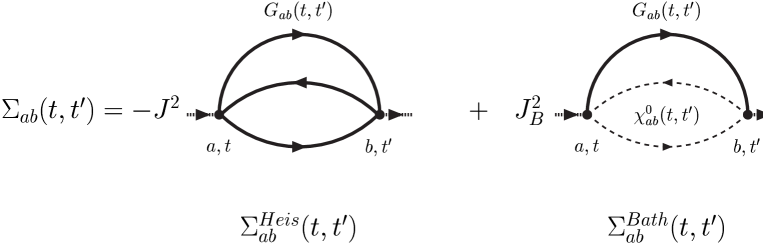Thus using Feynman rules in the $\pm$ representation, we find immediately (the factors can be checked against Matsubara computations : see appendix A) :

$$\Sigma_{ab}(t,t^{\prime})=-\underbrace{J^{2}abG_{ab}^{2}(t,t^{\prime})G_{ba}(t^{\prime},t)}_{\displaystyle\Sigma^{{\text{Heis}}}_{ab}(t,t^{\prime})}+\underbrace{\mathstrut J^{2}_{B}ab\chi_{ab}^{0}(t,t^{\prime})G_{ab}(t,t^{\prime})}_{\displaystyle\Sigma^{{\text{Bath}}}_{ab}(t,t^{\prime})}$$ (11)

We see that the bath only enters though its susceptibility $\chi^{0}$. For simplification, in the following, we take a specific form for the susceptibility of the bath $\chi^{0}_{ab}(t,t^{\prime})=G_{ab}^{0}(t,t^{\prime})G_{ba}^{0}(t^{\prime},t)$ where $G^{0}$ is the Green function of free fermions with a Lorentzian density of states at half filling (See section IV for a discussion on the relaxation bath and a justification of this formula).

To simplify the analysis of the dynamical equations, it is useful to write them in a different way, using the so-called “Larkin-Ovchinnikov representation” (LO) of the equations, in which the (matrix) Green function is given by

$$G=\frac{1}{2}\begin{pmatrix}1&1\\ 1&-1\end{pmatrix}\begin{pmatrix}G_{++}&G_{+-}\\ G_{-+}&G_{--}\end{pmatrix}\begin{pmatrix}1&1\\ -1&1\end{pmatrix}=\begin{pmatrix}R&K\\ 0&A\end{pmatrix}$$ (12)

where the retarded (response), advanced and Keldysh (correlation) two-times Green functions are defined by :

$$R(t,t^{\prime}) \equiv-i\theta(t-t^{\prime})\left\langle\bigl{[}b(t),b^{\dagger}(t^{\prime})\bigr{]}\right\rangle=G_{++}(t,t^{\prime})-G_{+-}(t,t^{\prime})$$ (13a)

$$A(t,t^{\prime}) \equiv+i\theta(t^{\prime}-t)\left\langle\bigl{[}b(t),b^{\dagger}(t^{\prime})\bigr{]}\right\rangle=G_{++}(t,t^{\prime})-G_{-+}(t,t^{\prime})$$ (13b)

$$K(t,t^{\prime}) \equiv-i\left\langle\bigl{\{}b(t),b^{\dagger}(t^{\prime})\bigr{\}}\right\rangle=G_{++}(t,t^{\prime})+G_{--}(t,t^{\prime})$$ (13c)

Note that our convention for $R$ differs from the one used for $R_{S}$. Moreover, we will use the relations :

$$A(t,t^{\prime}) =R(t^{\prime},t)^{*}$$ (14)

$$K(t,t^{\prime}) =-K(t^{\prime},t)^{*}$$ (15)

to eliminate $A$ and restrict ourselves to $t>t^{\prime}$. The (LO) representation is simpler because it uses the relation $G_{++}+G_{--}=G_{-+}+G_{+-}$ to reduce the number of functions (just $R$ and $K$, after that $A$ is eliminated using (14) and because it makes the causality of the equations explicit. In the (LO) representation the Keldysh indices structure of the vertices are particularly simple : the 2-leg vertex is $\delta_{ab}$ RammerSmith , which leads to a simple Dyson equation $G^{-1}=G^{-1}_{0}-\Sigma$ (where the inverse are just matricial inverses), and the four-leg vertex used in (11) is $(1\otimes\sigma_{x}+\sigma_{x}\otimes 1)/2$, where $1$ is the $2\times 2$ identity matrix and $\sigma_{x}$ is the usual Pauli matrix. Remarkably, this vertex factor is fully symmetric in the Keldysh space. Hence, a quick way to switch to the (LO) representation is to recompute the Feynman diagrams (See Figure (1)) with the (LO) Feynman rules (although a direct computation using just the definitions is possible but more tedious). After these manipulations, we finally obtain the main equations of our paper (for $t>t^{\prime}$) :

• The Dyson equations ((16c) is rewritten to involve only functions for $t>t^{\prime}$):

  $$i\partial_{t}R(t,t^{\prime}) =\delta(t-t^{\prime})+\int_{t^{\prime}}^{t}du\,\,\Sigma_{R}(t,u)R(u,t^{\prime})$$ (16a)

  $$i\partial_{t}K(t,t^{\prime}) =\int_{0}^{t}du\,\,\Sigma_{R}(t,u)K(u,t^{\prime})+\int_{0}^{t^{\prime}}du\,\,\Sigma_{K}(t,u)R^{*}(t^{\prime},u)$$ (16b)

  $$=\int_{t^{\prime}}^{t}du\,\,\Sigma_{R}(t,u)K(u,t^{\prime})+\int_{0}^{t^{\prime}}du\,\,\biggl{(}\Sigma_{K}(t,u)R^{*}(t^{\prime},u)-\Sigma_{R}(t,u)K^{*}(t^{\prime},u)\biggr{)}$$ (16c)

• The boundary conditions, which derive respectively from (2b) and the commutation relations of the boson :

  $$K(t,t) =-i(2S+1)$$ (16d)

  $$\lim_{t\rightarrow(t^{\prime})^{+}}R(t,t^{\prime}) =-i$$ (16e)

• The self-energy in LO representation (these formulas are local in times, so the argument $(t,t^{\prime})$ has been omitted for clarity) :

  $$\Sigma\equiv\Sigma^{{\text{Heis}}}+\Sigma^{{\text{Bath}}}$$ (16f)

  $$\Sigma_{R}^{{\text{Heis}}} \equiv-\frac{J_{H}^{2}}{4}\biggl{(}\Bigl{(}\big{|}R\big{|}^{2}-\big{|}K\big{|}^{2}\Bigr{)}R+\Bigl{(}R^{*}K-K^{*}R\Bigr{)}K\biggr{)}$$ (16g)

  $$\Sigma_{K}^{{\text{Heis}}} \equiv-\frac{J_{H}^{2}}{4}\biggl{(}\Bigl{(}\big{|}R\big{|}^{2}-\big{|}K\big{|}^{2}\Bigr{)}K+\Bigl{(}R^{*}K-K^{*}R\Bigr{)}R\biggr{)}$$ (16h)

  $$\Sigma_{R}^{{\text{Bath}}} \equiv\frac{J_{B}^{2}}{4}\biggl{(}\Bigl{(}\big{|}R_{0}\big{|}^{2}-\big{|}K_{0}\big{|}^{2}\Bigr{)}R+\Bigl{(}R^{*}_{0}K_{0}-K^{*}_{0}R_{0}\Bigr{)}K\biggr{)}$$ (16i)

  $$\Sigma_{K}^{{\text{Bath}}} \equiv\frac{J_{B}^{2}}{4}\biggl{(}\Bigl{(}\big{|}R_{0}\big{|}^{2}-\big{|}K_{0}\big{|}^{2}\Bigr{)}K+\Bigl{(}R^{*}_{0}K_{0}-K^{*}_{0}R_{0}\Bigr{)}R\biggr{)}$$ (16j)

where $R_{0}$ and $K_{0}$ are defined in the same way that $R$ and $K$ starting from $G^{0}_{a,b}$. This expression emphasizes the very similar structure of the two terms in the self-energy : more generally, the bath term reads $\Sigma_{R}^{{\text{Bath}}}\propto\chi^{0}_{K}R+\chi^{0}_{R}K$ and $\Sigma_{K}^{{\text{Bath}}}\propto\chi^{0}_{R}R+\chi^{0}_{K}K$, where $\chi^{0}_{R}$ and $\chi^{0}_{K}$ are the retarded and the Keldysh part of $\chi^{0}$ respectively.

Finally, we now derive the expression for the response and correlation functions for spins defined in (3). In the $N\rightarrow\infty$ limit, $C_{S}$ and $R_{S}$ can be easily computed from $R$ and $K$ using the relations :

$$R_{S}(t,t^{\prime}) =\frac{i}{N^{2}}\sum_{\alpha\beta}\Bigl{\langle}S^{+}_{\alpha\beta}(t)\left(S^{+}_{\beta\alpha}(0)-S^{-}_{\beta\alpha}(0)\right)\Bigr{\rangle}$$

$$=\hbox{Im}\left(K(t,t^{\prime})R^{*}(t,t^{\prime})\right)$$ (17a)

$$C_{S}(t,t^{\prime}) =\frac{1}{N^{2}}\sum_{\alpha\beta}\Bigl{\langle}S^{+}_{\alpha\beta}(t)S^{+}_{\beta\alpha}(0)-S^{-}_{\alpha\beta}(t)S^{-}_{\beta\alpha}(0)\Bigr{\rangle}$$

$$=\frac{1}{4}\Bigl{(}|K(t,t^{\prime})|^{2}-|R(t,t^{\prime})|^{2}-|R(t^{\prime},t)|^{2}\Bigr{)}$$ (17b)

To derive (17), we used Eqs. (2a,2b), the $SU(N)$ invariance, the limit $N\rightarrow\infty$ (to drop subdominant terms), and the relations between $G_{a,b}$ and $R,K,A$ that invert (13a).

The equations (16) describe the dynamics of the Quantum Heisenberg spin glass in the large-$N$ limit, coupled to the bath. In the following sections, we present an analysis of these equations both in the paramagnetic regime and in the aging regime, together with some results extracted from a numerical solution of this systems. Let us first make a few preliminary remarks :

• Contrary to the quantum $p-$spin problem studied in CugliandoloLozano , there is no need here for a Lagrange parameter associated to the constraint. This is due to the fact that the constraint (2b) commutes with the Hamiltonian and hence is conserved in the time evolution. Indeed one can check that (16g,16h,16i,16j) and (16a,16c) imply:

  $$\frac{dK(t,t)}{dt}\propto\hbox{Im}\frac{\partial}{\partial t}K\left.(t,t^{\prime})\right|_{t^{\prime}=t}=0$$ (18)

  Thus if the boundary condition is verified for $t=t^{\prime}=0$, it will propagate at all later times.

  Formally, one can introduce such a parameter $\lambda$ in the equation, by replacing $i\partial_{t}$ by $i\partial_{t}+\lambda$, but it can be removed using a $U(1)$ gauge transformation $[K(t,t^{\prime}),R(t,t^{\prime})]\rightarrow[\tilde{K}(t,t^{\prime}),\tilde{R}(t,t^{\prime})]=[e^{-i\lambda(t-t^{\prime})}K(t,t^{\prime}),e^{-i\lambda(t-t^{\prime})}K(t,t^{\prime})]$ : if $K,R$ are a solution of the equations with $\lambda$,$[\tilde{K},\tilde{R}]$ are a solution with $\lambda=0$. This symmetry comes from the fact that we represented the spin (the physical object) with the bosons (a mathematical tool) and that the bath couples to the spin and not to the boson, and thus can not break the symmetry; this has an important consequence (see ii).

• In equilibrium, the spin response and correlation functions are related by the quantum fluctuation dissipation relation QFDR:

  $$R_{S}(\tau)=i\theta(\tau)\int_{-\infty}^{+\infty}\frac{d\omega}{\pi}\exp(-i\omega\tau)\tanh\left(\frac{\beta\omega}{2}\right)C_{S}(\tau)$$ (19)

  It is important to notice that instead the boson response and correlation functions $R$ and $K$ are not in principle related by this QFDR. Technically, this is due to the $U(1)$ invariance explained above : if $[K(t,t^{\prime}),R(t,t^{\prime})]$ satisfies QFDR (19), $[\tilde{K},\tilde{R}]$ will not in general. Imposing QFDR for the boson demands that $\lambda$ takes a precise value $\lambda_{0}$. However, this is not a problem since the only physical objects are the spin response and correlation functions. When using the Matsubara imaginary time formalism, one does not face this difficulty, since one automatically requires the QFDR to be satisfied, because of the $\beta-$periodicity of the imaginary time boson Green function. Thus, when we will analytically continue our equations in imaginary time to compare to Matsubara computations (See Appendix A ), we will have to reintroduce $\lambda_{0}$.

• The presence of the thermal bath is clearly required : for $J_{B}=0$, the solution of the equations has the property $K(t,t^{\prime})=(2S+1)R(t,t^{\prime})$ for all $t,t^{\prime}$ (this can be check order by order in the coupling constants $J_{H}$ and $J_{B}$, using (16a,16c,16g,16h,16i,16j)) and it is clearly incorrect (for example, it can not satisfy the high-temperature limit of the fluctuation-dissipation relation).

• We can immediately generalize these equations in the fermionic case by changing $S\rightarrow-S,J_{H}^{2}\rightarrow-J_{H}^{2}$ ($S$ is the size of the “fermionic” spin, and the sign change in front of the coupling constant comes from the fact that there is now a fermion loop in the diagram). We will see in Section III that this simple change leads to the disappearance of the aging phenomena, as expected SachdevYe .

III Solutions of the dynamical equations

In this section, we present the solution of the dynamical equations (16) using both numerical and analytical results. Indeed, these integro-differential equations are causal, so one can construct the solution step by step in time. This property is very general (See CugliandoloLozano for another example) and it is the basis for the numerical algorithms, although in this problem some new technical refinements are needed in order to compute an accurate solution at a reasonable cost in computational time (see the appendix B for a detailed discussion). The numerical solution shows that the model has a dynamical phase transition at a temperature $T_{d}(S,J_{B})$ between a paramagnetic phase ($T>T_{d}$) and a glassy phase ($T<T_{d}$), as expected on general grounds and predicted in SGletter ; SGlong . At high temperature, the system equilibrates inside the paramagnetic state: after a transient time all the two-time quantities become time-translation invariant (TTI) and the quantum fluctuation dissipation relation QFDR holds. Instead at low temperature the system never equilibrates on finite timescales Note_FiniteTimescales and one can identifies two different time sectors on which the two-time functions evolve: when $t^{\prime}$ is large but the difference $t-t^{\prime}$ is of the order of one and very small compared to $t^{\prime}$ the system seems to be equilibrated (the QFDR is approximatively verified and all the one time quantities, as the energy or the Edwards-Anderson parameter, have almost converged to their asymptotic values). However, on larger timescales, when $t-t^{\prime}$ is of the same order of $t^{\prime}$, an extremely slow dynamics sets in. In this regime the QFDR is violated and the aging phenomenon appears CugliandoloLozano ; reviewDYN ; CugliandoloKurchanPRL . We remark that if one takes the long time limit and then sets the coupling to the bath to zero then the dynamical solution gets back to the equilibrium for $T>T_{d}$ only. For $T<T_{d}$ the system never reaches a stationary solution. However, the pseudo-equilibrium solution reached in the time sector $t-t^{\prime}\sim O(1)<<t^{\prime}$ can be also obtained by a pure static computation using the marginality prescription SGlong . In the following, we will take $J_{B}>0$ ($J_{B}=1$ for numerical computation). In section IV, we will discuss what happens changing the value of $J_{B}$.

III.1 Equilibration into the paramagnetic state

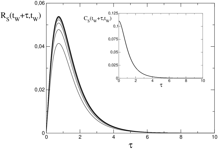
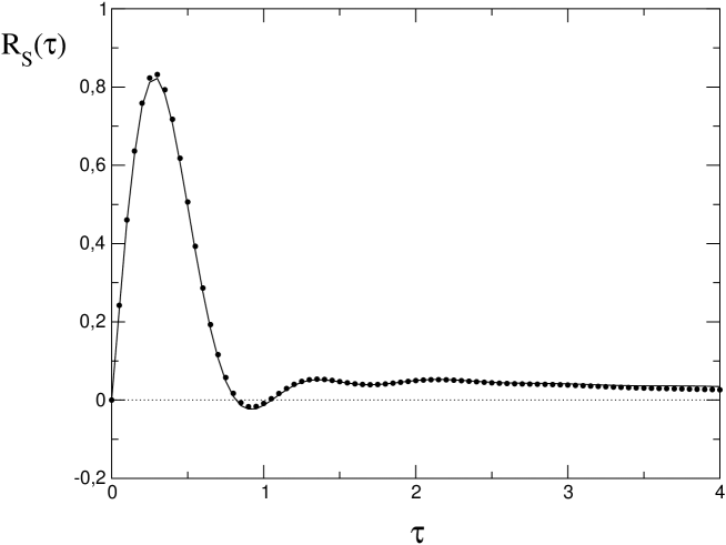
At high temperature, the numerical solution shows, as expected, that the system equilibrates into the paramagnetic state after a transient time $t_{eq}$: for $t,t^{\prime}>>t_{eq}$ the response and correlation becomes a function of $\tau=t-t^{\prime}$ only and they are related by the QFDR (see Fig. 2). This is indeed what we obtain from the analysis of Eqs. (16a,16c) in the limit $t,t^{\prime}\rightarrow\infty$ with $\tau=t-t^{\prime}$ fixed.

Figure 2: Spin response as a function of $\tau$ for $t_{w}=1.5,2,2.5,3,3.5,4,4.5,5,10,15,20,25$ (from bottom to top ($t_{max}=100$)), $J_{B}=J_{H}=1$, $S=1$ and $T=10$ (inside the paramagnetic phase). After a transient time the response converges to a stationary equilibrium regime. Inset: spin correlation as a function of $\tau$ for the same parameters.

In this limit the equation on $K$ and $R$ can be easily written in Fourier space (we reintroduce the $\lambda$ term, in agreement with the discussion at the end of section II):

$$R^{-1}(\omega) = \omega+\lambda-\Sigma_{R}(\omega)$$ (20a)

$$K(\omega) = \Sigma_{K}(\omega)|R(\omega)|^{2}$$ (20b)

Figure 3: Fourier transform of the spin response function (dots) compared to its expression (continuous line) computed by the QFDR from the correlation for $J_{B}=J_{H}=1$, $S=1$, $t_{W}>10$ and $T=10$ (inside the paramagnetic phase). The excellent agreement shows that the system is fully equilibrated.

As in CugliandoloLozano , it is possible to show order by order in perturbation theory that these equations admit a solution such that the spin correlation and response functions satisfy QFDR. In Figure 2, we plot the spin correlation function $C_{S}(t_{w}+\tau,t_{w})$ and the response function $R_{S}(t_{w}+\tau,t_{w})$ as a function of $\tau$ for different $t_{w}$ for $J_{B}=1$, $J_{H}=1$ and $T=10$. These figures represents the typical behavior of $C_{S}$ and $R_{S}$ in the paramagnetic phase: after a short transient time the functions become TTI (they do not depend on $t_{w}$ anymore) and they decay quickly as a function of $\tau$. 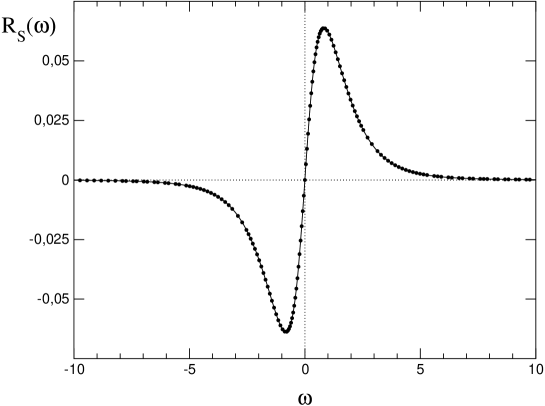Moreover, in Figure 3, we plot the retarded function computed directly from the numerical solution and from the correlation function using the QDFR. The excellent agreement shows that QFDR is satisfied and the system has relaxed to equilibrium.
This asymptotic solution represent the equilibrium dynamics inside the paramagnetic state and it exist only above $T_{d}$. At $T=T_{d}$ the equilibration time diverges and remains infinite in all the low temperature phase ($T<T_{d}$), as clearly indicated by the numerical solution (see Fig. 4). The study of this regime is the subject of the next subsections.

In principle, one would like to take a small $J_{B}$, so that it allows the system to relax but does not change the value of the paramagnetic state. However, the relaxation time diverges when $J_{B}$ goes to 0, even in the paramagnetic state, and this prevent the numerical program to converge towards the solution in a reasonable amount of time. We found that $J_{B}=1$ is a good compromise. Indeed the imaginary time computation shows that the results at $J_{B}=0$ are close to $J_{B}=1$. This relatively big value reflects the fact our bath, coupling to the spin degrees of freedom, is not very efficient. A more precise discussion will be given in Section IV.

III.2 General properties of the glassy dynamics

The numerical results and the analytical analysis of the dynamical equations indicates that the system remains always out of equilibrium at low temperature ($T<T_{d}$). In the following we present the Ansatz which gives the asymptotic solution in the glassy regime and we compare it to the numerical results obtained integrating the dynamical equation numerically. This Ansatz is a slight generalization of the one introduced by Cugliandolo and Lozano CugliandoloLozano for quantum glassy systems, which is itself a generalization of the one discovered by Cugliandolo and Kurchan for classical glassy systems CugliandoloKurchanPRL .

III.2.1 The weak-ergodicity breaking and the weak long-term memory Ansatz

In the long time limit ($t,t^{\prime}>>1$) we make the following Ansatz for the behavior of the bosonic correlation and response function CugliandoloLozano :

$$K(t,t^{\prime}) \simeq\left[K_{ST}(t-t^{\prime})+K_{AG}\left(\frac{h(t^{\prime})}{h(t)}\right)\right]e^{-i\lambda(t-t^{\prime})}$$ (21a)

$$R(t,t^{\prime}) \simeq\left[R_{ST}(t-t^{\prime})+\frac{h^{\prime}(t^{\prime})}{h(t)}R_{AG}\left(\frac{h(t^{\prime})}{h(t)}\right)\right]e^{-i\lambda(t-t^{\prime})}$$ (21b)

$$\lim_{t\rightarrow\infty}K_{ST}(t) =0$$ (21c)

$$K_{ST}(0) =-i(2S+1)+ig$$ (21d)

$$K_{AG}(0) =0$$ (21e)

$$K_{AG}(1) =-ig$$ (21f)

where $h(t)$ is an increasing function of $t$, $h^{\prime}(t)$ is the first derivative of $h(t)$, $g$ is a real number Note_EA and $g^{2}/4$ is equal to the Edwards-Anderson parameter $q_{EA}$. Note the physics hidden in this Ansatz: in the time regime in which $t,t^{\prime}$ are large but their difference remains finite (called TTI-regime in the following) the system seems to have reached a stationary state, however on a timescale diverging with $t,t^{\prime}$ ($t,t^{\prime}$ are large but the ratio $h(t^{\prime})/h(t)$ remains finite) there is a secondary evolution called aging reviewDYN . This unveils the interpretation of $h(t)$ as a self-generated effective time scale.

Moreover we notice that if this scenario is realized for the bosonic correlation and response functions then it will be also realized for the spin correlation and response functions and for the self-energies. The presence of the oscillating exponential is a slight generalization with respect to CugliandoloLozano and it could be gauged away, as discussed before. Moreover, when one compute the spin correlation and response functions these exponentials cancel.

The second key ingredient that makes the asymptotic problem tractable is the assumption of the weak long-term memory property CugliandoloLozano ; CugliandoloKurchanPRL that allows one to decouple the transitory regime from the asymptotic one. In fact the dynamical equations contains explicitly memory terms which couple all the timescales. So, how can one analyze the asymptotic regime without solving the complete problem? Within the weak long-term memory scenario the (linear) response to a finite time perturbation vanishes in the long time limit ($t,t^{\prime}\rightarrow\infty$), whereas the response to a perturbation which acts on infinite timescales (i.e. diverging as $t,t^{\prime}$) is finite. More precisely:

$$\lim_{t\rightarrow\infty}\int_{0}^{t^{*}}R(t,u)f(u)du=0\qquad{\mbox{but}}\qquad\lim_{t\rightarrow\infty}\int_{0}^{t}R(t,u)f(u)du\neq 0\quad,$$ (22)

where $f(t)$ is a generic function. Therefore the dynamics on “infinite timescales” ($t,t^{\prime}\rightarrow\infty$) decouples from the transitory regime.
Finally, we note that more general Ansätze with a set of different diverging timescales have been used in the context of classical CugliandoloKurchanPhilMag ; FranzMezard and quantum ChamonRotors glassy systems. However, this type of solutions are physically and technically related to a full replica symmetry breaking solution in the thermodynamical analysis. For systems characterized by a one step replica symmetry breaking solution in the thermodynamics, as the model we are focusing on SGletter , one generally expects only one diverging timescale.

III.2.2 Generalized QFDR

An outstanding physical property of the asymptotic dynamical solutions, discovered in the classical case by Cugliandolo and Kurchan CugliandoloKurchanPRL and in the quantum case by Cugliandolo and Lozano CugliandoloLozano , is that in the aging time-sector ($t$, $t^{\prime}$ and $t-t^{\prime}$ are large but the ratio $h(t^{\prime})/h(t)$ stays finite) the standard fluctuation dissipation relation is violated but there exists a generalized fluctuation dissipation relation (GFDR) between the correlation and the response functions which has the usual functional form of the FDR (generalized to non TTI functions) and in which the temperature $T$ is replaced with an effective temperature $T_{\text{eff}}$ CugliandoloLozano . Two remarks are in order concerning $T_{\text{eff}}$. First, a physical one: the effective temperature has a real physical meaning of temperature effectivetemp since is what a thermometer, whose reaction time equals the timescales on which the aging evolution takes place, would measure. Second, a technical one. The effective temperature $T_{\text{eff}}$ is related to the breaking point $x$ arising in the replica symmetry breaking solution of the thermodynamics, i.e. $T_{\text{eff}}=T/x$. A general argument to show why one expects this to be true for a very large class of classical systems, included finite dimensional systems, has been presented in FranzMezardParisiPeliti .
It is important to note, as pointed out in CugliandoloLozano that in the quantum case the GFDR is expected to become classical. The argument is the following: if $T_{\text{eff}}$ is finite then the Fourier integral relating the correlation and the response is dominated by $\omega\propto 0$. Hence, one can develops the hyperbolic tangent recovering back a classical generalized fluctuation dissipation relation, which in our case (for spins) reads:

$$R_{S}(t,t^{\prime})=\frac{1}{T_{\text{eff}}}\partial_{t^{\prime}}C_{S}(t,t^{\prime})$$ (23)

This becomes a relation between the aging functions:

$$R^{AG}_{S}(\mu)=\frac{1}{T_{\text{eff}}}(C^{AG}_{S})^{\prime}(\mu)$$ (24)

where $\mu=h(t^{\prime})/h(t)$. Moreover this has been argued to be generically true for models with simple commutation relations (particles and rotors) in ChamonRotors since the dynamical equations are fixed point of the re-parameterization group of time transformations and the renormalized aging dynamics becomes classical at the fixed point. The quantum mechanics enters only as a renormalization of the coefficients of the dynamical equations. We will show that this is also the case for our system which is characterized by non trivial commutation relations between the spins (contrary to the case of rotors or particles). However, the behavior next to the quantum critical point is still unclear (See section V).

III.3 Numerical results

Figure 4: Spin correlation as a function of $\tau$ for $t_{w}=15,20,\dots,95$ (from bottom to top ($t_{max}=100$)), $J_{B}=J_{H}=S=1$ and $T=0.1$ (inside the glassy phase). The height of the dotted straight line equals the Edwards-Anderson parameter computed within the static formalism and coincides well with the plateau value. The aging behavior is explicit. Inset: zoom of the spin correlation as a function of $\tau$ on the time interval corresponding to the stationary regime for $t_{w}=5,10,25,37.5,50,75$ from bottom to top. The curves show a clear convergence toward a TTI stationary regime.

The numerical procedure used is described in Appendix B. It turns out that the problem is more difficult to solve than the classical ones or the quantum $p-$spins model, because the dynamical equations are for the auxiliary boson $b$ and not directly for the physical spin $S$.

Figure 5: Spin response as a function of $\tau$ for $t_{w}=5,10,25,37.5,50,75$ (from top to bottom ($t_{max}=100$)), $J_{B}=J_{H}=S=1$ and $T=0.1$ (inside the glassy phase). Inset: zoom of the integrated response as a function of $\tau$ on the time interval corresponding to the stationary regime for $t_{w}=5,10,25,37.5,50,75$ from bottom to top. The aging behavior and the weak long term memory scenario are explicit.

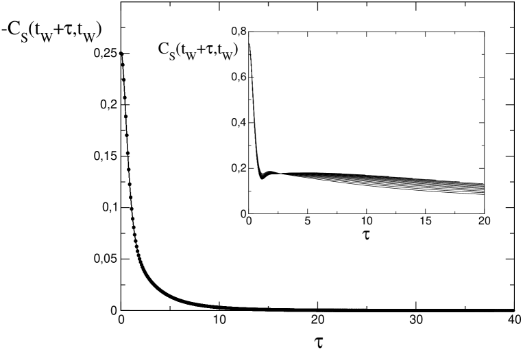
As clearly indicated in the Ansatz, even in the aging time-regime where the spin correlation and response function evolve very slowly, the bosonic functions oscillate wildly.

Figure 6: Parametric plot of the spin integrated response as a function of $C_{S}$ for $t_{w}=40,45,55,60,65,70$ ($t_{max}=100$), $J_{B}=J_{H}=S=1$ and $T=0.1$ (inside the glassy phase). The collapse predicted by the dynamical Ansatz is good. The vertical dotted straight line indicates the values of the Edwards-Anderson computed within the static formalism. The dashed straight line has a slope $-1/T_{\text{eff}}$ where $1/T_{\text{eff}}=x/T$ and $x$ has been computed within the static formalism. The curves clearly show that the generalization of the fluctuation dissipation relation holds in the aging regime.

The numerical solution thus demands a more sophisticated algorithm, inspired from well-known methods to solve one variable differential equations.
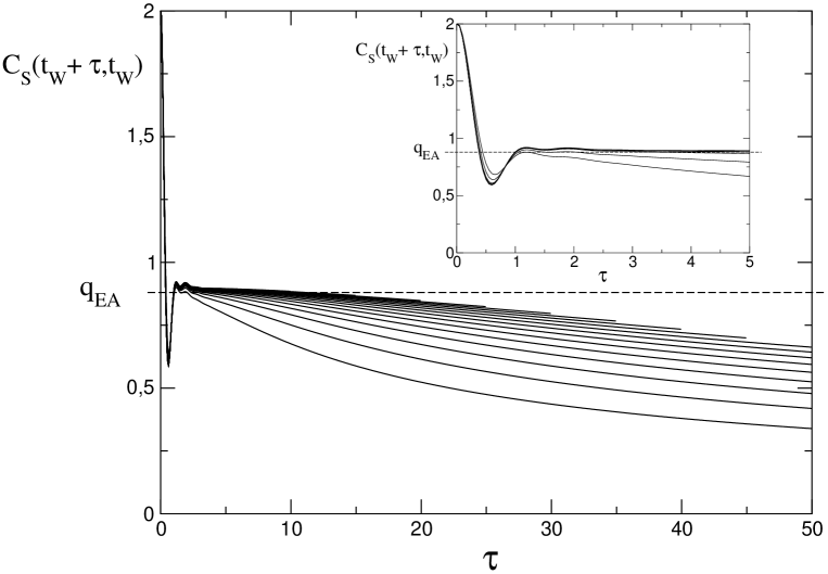
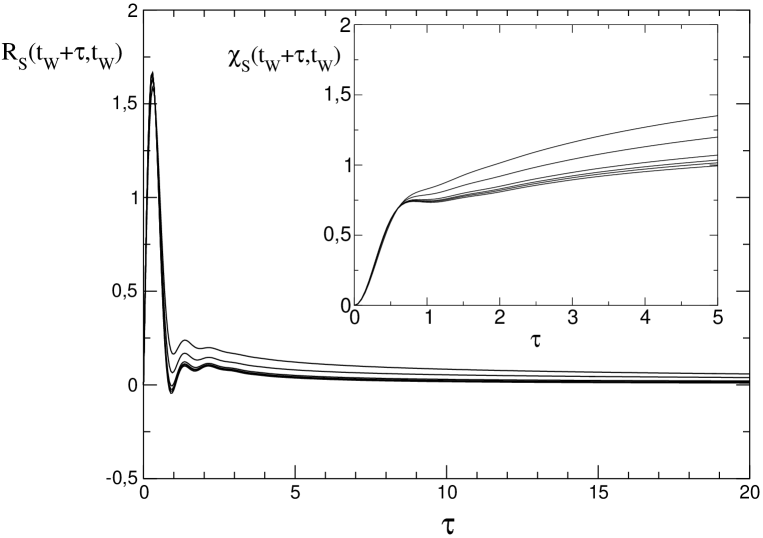
The numerical results support and validate completely the out of equilibrium scenario encoded in the Ansatz (III.2.1). In the following we present the results for $J_{H}=1$, $J_{B}=1$ and a temperature well inside in the glassy phase $T=0.1$. In Fig. 4, we plot respectively the spin correlation function $C_{S}(t_{w}+\tau,t_{w})$ and the spin integrated response function $\chi(t_{w}+\tau,t_{w})=\int_{t_{w}}^{t_{w}+\tau}dsR_{S}(t_{w}+\tau,s)$ as a function of $\tau$ for different values of $t_{w}$. We remark that a pseudo stationary regime sets in for $\tau<1$ with a plateau, whose height is the Edwards-Anderson parameter. Its value ($q_{EA}^{st}\simeq 0.88$), computed from the static analysis by the marginality prescription, is represented with a dashed line on Figure 4 : this shows a very good agreement between the two methods.

Figure 7: Spin correlation as a function of $\tau/t_{w}$ for $t_{w}=15,20,\dots,95$ (from bottom to top ($t_{max}=100$)), $J_{B}=J_{H}=S=1$ and $T=0.1$. These are the same curves plotted in Fig. 4 but with respect to the variable $\tau/t_{w}$. The excellent collapse strongly suggests that the function $h(t)$ (present in the dynamical Ansatz) should be equal to $t$.

Moreover the fact that correlation and response are related by the QFDR in this time sector, see Fig. 8, shows nicely that this is indeed a pseudo-equilibrium regime.

Figure 8: TTI part of the spin response function (dots) compared to its expression (continuous line) computed by the QFDR from the correlation for $J_{B}=J_{H}=1$, $S=1$, $t_{W}>10$ and $T=0.1$.

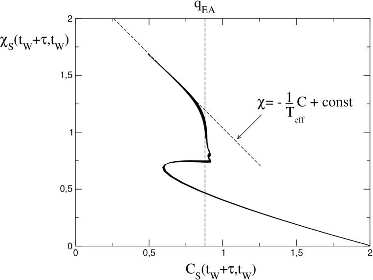
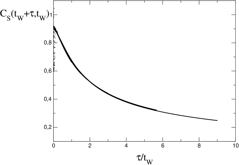
On a longer timescale $\tau\propto t_{w}$ the aging behavior sets in as clearly indicated in the two figures. The integrated response and the correlation evolve more and more slowly increasing $t_{w}$. Note that the behavior of $\chi$ shows explicitly the weak long term memory scenario: even if the response vanish in the aging time sector the integrated response does not. Therefore the magnetization response to a constant and small magnetic field switched on at $t_{w}$ depends always explicitly on $t_{w}$ and becomes slower increasing $t_{w}$. Moreover we note that the numerical results strongly suggest that $h(t)=t$. Indeed the different curves $C_{S}(t_{w}+\tau,t_{w})$ collapse very well on a single curve ($K_{AG}(\mu)$) when plotted as a function of $(t_{w}+\tau)/t_{w}$, see Fig. 7. We have also verified the correctness of the GFDR hypothesis. In Fig. 6, we show a parametric plot of $\chi$ as a function of $C_{S}$ for different values of $t_{w}$. For classical systems reviewDYN the limiting curve (for $t_{w}\rightarrow\infty$) is very useful to characterize the aging behavior. For systems with only one diverging timescale, because of the form of the FDR and the GFDR, one finds a two straight line plot where $\chi\propto-\frac{1}{T}C_{S}$ for $q_{EA}<C_{S}<C(t,t)$ and $\chi\propto-\frac{1}{T_{eff}}C_{S}$ for $0<C_{S}<q_{EA}$. In the quantum case the situation is more involved since in the stationary regime $R_{S}$ and $C_{S}$ are related by the QFDR, therefore one does not expect that for $q_{EA}<C_{S}<K(t,t)$ the plot should be very useful. However, as discussed in CugliandoloLozano , in the aging time sector where $0<C_{S}<q_{EA}$ the GFDR becomes classical and one should recover a straight line for $\chi$ whose slope equals the inverse of the effective temperature. This is indeed what we find in Fig. 6, where we compare the behavior of $\chi$ at low $C_{S}$ with a straight line whose slope is $1/T_{\text{eff}}=x/T$.

Figure 9: Spin correlation as a function of $\tau$ in the fermionic case for $t_{w}=12,14,\dots 48$ ($t_{max}=100$), $J_{B}=J_{H}=1$, $S=0.5$ and $T=0.1$. Inset: Spin correlation as a function of $\tau$ in the bosonic case for the same value of the parameter. This figure clearly shows the existence of aging in the bosonic case and its absence in the fermionic one.

$x$ is the breakpoint in the one-step replica symmetry breaking solution obtained (for the same value of the parameters) generalizing the analysis performed in SGletter to taking into account the presence of the bath (see Appendix A).

Finally, we can obtain the equations for the fermionic model by the simple change $S\rightarrow-S,J_{H}^{2}\rightarrow-J_{H}^{2}$ in (16) as discussed previously. Numerically solving these equations we have found no glassy behavior as predicted in SachdevYe . Indeed we show in Fig. 9 the spin correlation function in the fermionic case, which does not show any aging behavior at low temperature, whereas the same calculation for bosons (with the same parameters) clearly does.

III.4 Analysis of the stationary regime

We focus now on the time sector in which the difference between $t$ and $t^{\prime}$ stays finite and $t,t^{\prime}$ are very large. Hence, in Eqs. (21a,21b) the aging part does not evolve and is zero for the response and equals $-ig$ for the correlation. Plugging the Ansatz (21a,21b) into the dynamical equations we get:

$$(i\partial+\lambda)R_{ST}(t) = \int_{0}^{t}dt^{\prime}\Sigma_{R}^{ST}(t-t^{\prime})R_{ST}(t^{\prime})+\delta(t)$$ (25)

$$(i\partial+\lambda)K_{ST}(t) = \int_{-\infty}^{+\infty}dt^{\prime}\Sigma_{R}^{ST}(t-t^{\prime})K_{ST}(t^{\prime})+\int_{-\infty}^{+\infty}dt^{\prime}\Sigma_{K}^{AG}(t+t^{\prime})R_{ST}^{*}(t^{\prime})+A$$ (26)

$$A = \lim_{t\rightarrow\infty}\int_{0}^{t}du\frac{h^{\prime}(u)}{h(t)}\Sigma_{R}^{AG}\left(\frac{h(u)}{h(t)}\right)K_{AG}\left(\frac{h(t)}{h(u)}\right)+\lim_{t\rightarrow\infty}\int_{0}^{t}du\Sigma_{K}^{AG}\left(\frac{h(u)}{h(t)}\right)\frac{h^{\prime}(u)}{h(t)}R_{AG}^{*}\left(\frac{h(u)}{h(t)}\right)$$ (27)

$$-ig\int_{0}^{\infty}dt^{\prime}\Sigma_{R}^{ST}(t^{\prime})+\Sigma_{K}^{\infty}\int_{0}^{\infty}dt^{\prime}R^{ST}(t^{\prime})+i\lambda g$$

where we have used for the self-energy the same notation introduced in (21a,21b), and $\Sigma_{K}^{\infty}=\Sigma_{K}^{AG}(1)$. Since we have defined $K_{ST}(t)$ in such a way that it vanishes in the long time limit, $A$ has to be equal to zero. Note that this overall equation couples the stationary and the aging regime. As in the paramagnetic case, one can show (order by order in perturbation theory) that $R_{ST}$ and $K_{ST}$ satisfy the QFDR (and therefore $R_{S}^{ST},C_{S}^{ST}$ too). It could seem that the procedure to fix $\lambda$ is different in the two cases. In fact in the paramagnetic case one chooses $\lambda$ in such a way that the QFDR is verified for bosonic functions, instead now $\lambda$ is such that the correlation and response functions do not oscillate in the large time limit when $t-t^{\prime}$ and $t,t^{\prime}$ are very large. But the two values of $\lambda$ are the same an asymptotically oscillating function cannot satisfy the QFDR relation.

As a conclusion the stationary equations can be fully interpreted as equilibrium dynamical equations. Indeed it has been shown in the classical CugliandoloKurchanPRL and recently in the quantum case QuantumTAP that this type of equations represents the pseudo-equilibrium relaxation inside the marginally stable TAP states (local minima of the free energy landscape whose Hessian is characterized by a vanishing fraction of zero modes). Imposing the marginality condition in the static computation SGlong is equivalent to consider a Boltzmann measure restricted to the marginally stable TAP states. It is for this reason that one can get information about the out of equilibrium dynamics by a purely equilibrium computation. However, it is important to understand that the equations (25,26,27) do not really represent an equilibrium relaxation. Because the marginally stable TAP states have a vanishing fraction of zero modes, the system find always a way to “escape” to these states, even if more and more slowly and this gives rise to the aging behavior. Hence, the physical mechanism inducing the slow dynamics is not an activated jump dynamics across some energy barriers but it is an entropic effect. The slow dynamics of the system is due to the fact that the longer is the time the smaller is the number of directions along which the system can escape. Finally, the fact that the marginally stable TAP states dominate the off-equilibrium dynamics whereas they are not relevant for equilibrium properties helps to understand why the dynamical transition temperature is different from (actually is larger than) the equilibrium transition temperature. In fact after a quench, the system is almost trapped in those minima and thus displays the aging phenomenon at long time. The local minima responsible for the slow dynamics appear at a temperature higher than $T_{eq}$, thus $T_{d}>T_{eq}$. The activated dynamics which would probably restore the equality $T_{d}=T_{eq}$ is on timescales diverging with $N$, completely unaccessible to our mean-field analysis.

III.5 Analysis of the aging regime

Let us now focus on the aging regime, i.e. $t$, $t^{\prime}$ and also $t-t^{\prime}$ are large but the ratio $h(t^{\prime})/h(t)$ stays finite. Note that within the following asymptotic analysis one cannot find out what is the function $h(t)$ CugliandoloKurchanPRL ; CugliandoloLozano ; ChamonRotors . This is indeed an open problem already for classical systems. However, the numerical results, see FIG. 7, suggest that for our model $h(t)=t$.

Plugging the Ansatz (21a,21b) into the dynamical equations and after some manipulations similar to CugliandoloLozano we get:

$$\lambda R_{AG}(\mu)= \int_{\mu}^{1}\frac{dx}{x}\Sigma_{R}^{AG}(x)R_{AG}\left(\frac{\mu}{x}\right)+\Sigma_{R}^{ST}(\omega=0)R_{AG}(\mu)+\Sigma_{R}^{AG}(\mu)R_{ST}(\omega=0)$$ (28)

$$\lambda K_{AG}(\mu)= \int_{0}^{\mu}\frac{dx}{\mu}\Sigma_{K}^{AG}(x)R_{AG}^{*}\left(\frac{x}{\mu}\right)+\int_{0}^{1}dx\Sigma_{R}^{AG}(x)K_{AG}\left(\frac{\mu}{x}\right)+\Sigma_{R}^{ST}(\omega=0)K_{AG}(\mu)$$

$$+\Sigma_{K}^{AG}(\mu)R_{ST}^{*}(\omega=0)$$ (29)

$$\Sigma_{R}^{AG}(\mu)= -\frac{J_{H}^{2}}{4}\left(K_{AG}^{2}(\mu)R_{AG}^{*}(\mu)-2|K_{AG}(\mu)|^{2}R_{AG}(\mu)\right)$$ (30)

$$\Sigma_{K}^{AG}(\mu)= \frac{J_{H}^{2}}{4}|K_{AG}(\mu)|^{2}K_{AG}(\mu)$$ (31)

where $K_{AG}$ satisfies the boundary condition $K_{AG}(1)=-ig$ and we have used the notation $\mu=h(t^{\prime})/h(t)$. It is important to remark that:

1. there is no bath contribution to the aging part of the self-energy. This is natural and it is probably generally true since the bath has always its own equilibration timescale, therefore in the aging time-sector ($t$, $t^{\prime}$ and $t-t^{\prime}$ are large but the ratio $h(t^{\prime})/h(t)$ stays finite) the bath is always already equilibrated and cannot give a non-constant aging contribution.

2. the terms linear in $R$ (and higher) have been neglected in $\Sigma_{K}^{AG}$, whereas the terms quadratic (and higher) have been neglected in $\Sigma_{R}^{AG}$. This is due to the fact that they do not give a finite contribution in the aging equations.

3. As pointed out in the classical case CugliandoloKurchanPRL and recently in the quantum case ChamonRotors the equations (28,29,30,31) are re-parameterization invariant. However there is only one function $h(t)$ reached by the system in the long time limit. This is a general problem arising in the study of the asymptotic solution of partial and integro-differential equations, called the matching problem. Until now different techniques are known and applied to solve this problem for partial differential equations but its solution for the dynamical equations arising in the study of glassy systems remains an open problem.

4. The correlation and response functions are supposed to be related by the GFDR in the aging regime after that the exponential $e^{-i\lambda(t-t^{\prime})}$ has been gauged out. In particular the GFDR predicts that $R_{AG}(\mu)=-\frac{i}{2T_{\text{eff}}}(K_{AG})^{\prime}(\mu)$ (in our notation the GFDR for bosons has a $-i/(2T_{\text{eff}})$ instead that $1/T_{\text{eff}}$). One can indeed verify that this is really a property of the aging equations: (28) can be obtained by differentiating (29) and using the GFDR. Moreover, we remark that if the bosonic correlation and response functions verify the GFDR so do the spin correlation and response functions as in (24) : $T_{\text{eff}}$ is the effective temperature.

Evaluating the aging equations in $\mu=1$ and imposing the existence of an aging solution, i.e. $R_{AG}(1)\neq 0$ we obtain two matching conditions with the stationary regime CugliandoloLozano : the first one is

$$\lambda=\Sigma_{R}^{ST}(\omega=0)+\left.\frac{\Sigma_{R}^{AG}}{R_{AG}}\right|_{\mu=1}R_{ST}(\omega=0)$$ (32)

and the second is the same one already obtained from the long-time limit of the stationary equation, i.e. $A=0$, (eq. (27)). One can simplify further these two matching equations. Indeed, thanks to the GFDR (24), one can perform the integrals on the aging functions in $A$. Hence, using the zero frequency term of (25), we get:

$$\frac{J_{H}^{2}}{4}R_{ST}^{2}(\omega=0)g^{2}\left(\left.\frac{R_{AG}^{*}}{R_{AG}}\right|_{\mu=1}+2\right) = 1$$ (33)

$$\frac{i}{2T_{\text{eff}}}\Sigma_{K}^{\infty}g-\frac{ig}{R_{ST}(\omega=0)}-\Sigma_{K}^{\infty}R_{ST}^{*}(\omega=0) = 0$$ (34)

Moreover, because $R_{ST}$ is a bosonic response function in a pseudo-equilibrium regime, its zero frequency component is real and negative. Therefore $\left.\frac{R_{AG}^{*}}{R_{AG}}\right|_{\mu=1}$ is a real number equal to one or minus one that we will note $\zeta$ in the following and $R_{ST}(\omega=0)$ reads:

$$R_{ST}(\omega=0)=-\frac{2}{J_{H}g\sqrt{2+\zeta}}$$ (35)

Plugging this expression onto (34) and using that $\Sigma_{K}^{\infty}=-i\frac{J^{2}_{H}}{4}g^{3}$ we finally obtain the equation for $T_{\text{eff}}$. The aging solution corresponds to $\zeta=+1$ ($\zeta=-1$ implies $g^{2}/T_{\text{eff}}=0$) and is characterized by the following equation:

$$\frac{J_{H}q_{EA}}{T_{\text{eff}}}=\left(\sqrt{3}-\frac{1}{\sqrt{3}}\right)$$ (36)

where we have replaced $g^{2}=4q_{EA}$. Note that, replacing $T_{\text{eff}}$ with $T/x$ (where $x$ is the breakpoint in the one-step replica symmetry breaking scheme) this becomes the same equation obtained in SGletter using the marginality condition.
Indeed (25,26) with $A=0$ and (35,36) and the boundary condition $K_{ST}(\tau=0)=-i(2S+1)+ig$ are a closed set of equations that completely determines $K_{ST},R_{SR},\lambda,T_{\text{eff}},q_{EA}$. In Appendix A, we show that they are completely equivalent to the equations studied in SGletter ; SGlong using the marginality prescription within a pure static computation. Finally, let us stress that, even if $J_{B}$ is not present in eq. (36), $T_{\text{eff}}$ depends on $J_{B}$ because the Edwards-Anderson parameter depends on $J_{B}$ via the eqs. (25,26) which contains explicitly this coupling constant.

IV Role of the relaxation bath

In this section, we briefly discuss the effect of the coupling strength to the relaxation bath $J_{B}$. In deriving Eqs (16), we took a generic bath and expand in second order in its coupling constant $J_{B}$. Thus the equations we derived are a priori only valid in the limit of small $J_{B}$. However, we will show that our main equations (16) also describe the dynamics of a model with finite $J_{B}$ in a extreme limit. Thus it is legitimate to study them for $J_{B}$ finite (there is no risk of inconsistencies).

The effect of the bath will of course depend on its precise form. Two types of bath can be considered : baths that only couple to the spin, and baths that couple to the boson or the fermions. In this discussion, we will concentrate on the first kind, since the spin is the physical object, not the boson. One of the simplest possibility is to couple the spin to 2 fermions using the Kondo interaction. In order to take the large-$N$ limit, we directly introduce the $SU(N)\times SU(N\gamma)$ Kondo model, with $N\gamma$ flavors, defined by ParcolletGeorgesPRLKondo+ParcolletGeorgesKotliarSengupta :

$$H=\frac{1}{\sqrt{{\cal N}N}}\sum_{i<j}J_{ij}\vec{S}_{i}\cdot\vec{S}_{j}+\sum_{\begin{subarray}{c}k\\ 1\leq i\leq N\gamma\\ 1\leq\alpha\leq N\end{subarray}}\epsilon_{k}c^{\dagger}_{ki\alpha}c_{ki\alpha}+\frac{J_{B}}{N\sqrt{\gamma}}\sum_{\begin{subarray}{c}1\leq\alpha,\beta\leq N\\ 1\leq i\leq N\gamma\end{subarray}}S_{i\alpha\beta}c^{\dagger}_{ki\beta}c_{k^{\prime}i\alpha}$$ (37)

where $c$ are the bath fermions, $\epsilon_{k}$ their kinetic energy and $J_{B}$ is now the Kondo coupling. In the large-$N$ limit, one can still find a closed system of equations, but at the expense of introducing auxiliary fermionic Green functions $r$ and $k$, as explained for example in ParcolletGeorgesPRLKondo+ParcolletGeorgesKotliarSengupta . The dynamical equations are similar to (16) : (16a,16b,16d) are the same and the bath term in self energies (16i,16j) are replaced by :

$$\Sigma_{R} =-\frac{J_{H}^{2}}{4}\biggl{(}\Bigl{(}K^{2}+R^{2}\Bigr{)}R^{*}-2|K|^{2}R\biggr{)}-\frac{i\sqrt{\gamma}J_{B}}{2}\biggl{(}R_{0}^{*}k-K_{0}^{*}r\biggr{)}$$ (38a)

$$\Sigma_{K} =-\frac{J_{H}^{2}}{4}\biggl{(}2K|R|^{2}-K^{*}\Bigl{(}R^{2}+K^{2}\Bigr{)}\biggr{)}-\frac{i\sqrt{\gamma}J_{B}}{2}\biggl{(}R_{0}^{*}r-K_{0}^{*}k\biggr{)}$$ (38b)

Since the bath has now a proper dynamics, $r$ and $k$ should be computed using new Dyson equations :

$$r(t,t^{\prime}) =\delta(t-t^{\prime})+\int_{t^{\prime}}^{t}du\;\sigma_{R}(t,u)r(u,t^{\prime})$$ (39a)

$$k(t,t^{\prime}) =\int_{0}^{t}du\,\,\sigma_{R}(t,u)k(u,t^{\prime})+\int_{0}^{t^{\prime}}du\,\,\sigma_{K}(t,u)r(t^{\prime},u)^{*}$$ (39b)

and their self-energy reads:

$$\sigma_{R}^{\text{Heis}} =\frac{iJ_{B}}{2\sqrt{\gamma}}\biggl{(}R_{0}K+K_{0}R\biggr{)}$$ (40a)

$$\sigma_{K}^{\text{Heis}} =\frac{iJ_{B}}{2\sqrt{\gamma}}\biggl{(}R_{0}R+K_{0}K\biggr{)}$$ (40b)

$r$ should also satisfy the boundary condition :

$$\lim_{t\rightarrow(t^{\prime})^{+}}r(t,t^{\prime})=-i$$ (41)

It is not difficult to show that in the limit of an infinite number of channel $\gamma\rightarrow\infty$, these equations reduce to (16).

However, for finite $\gamma$, these equations are much more complex than (16), since at low temperature the Kondo scale appears and one has to deal with a problem with many different scales. This really increases the difficulty of a numerical computation. However, one can extend rather simply the previous analytical study and verify that the same dynamical scenario continues to hold. In this paper, we restricted ourselves to study (16) as a function of the strength of the bath $J_{B}$, using Matsubara formalism with marginality condition SGlong . We found that increasing $J_{B}$ the spin glass transition temperature $T_{g}$ decreases monotonically and as far as we can solve the numerical equations, the transition is still second order, given by the condition $x=1$ ($x$ is the value of the breakpoint in the replica formalism). However, the decrease of $T_{g}$ is slow and we could not reach numerically a point where it vanishes. Numerical computation can not for the moment decide whether there is a second order phase transition until a quantum critical point at finite $J_{B}$ and $T=0$ or the spin glass is not destroyed at zero temperature until $J_{B}=\infty$. As emphasized in our concluding remarks, this situation is disappointing since we would like to study the aging in the vicinity of a non pathological quantum critical point for this model. Our interpretation is that this bath, coupled to the spin directly, is not “efficient” enough and that we probably need to couple to a bath with charge fluctuations by introducing holes in the model. Such a doped model is also interesting physically to study the destruction of a quantum spin glass by doping. Finally, let us emphasize that solving numerically the model with the Kondo bath (37) or a more general bath may lead to more interesting results, such as an increase of the critical temperature and the Edwards-Anderson parameter as the coupling to the bath increases from 0 GrempelCugliPRIVATE .

V Summary and discussion

In this paper we have studied the out of equilibrium dynamics of the quantum Heisenberg spin glass defined on a completely connected lattice and coupled to a spin thermal bath. We have replaced the $SU(2)$ spin symmetry group with $SU(N)$ and we have considered the large-$N$ limit. This has allowed us to have a more tractable model which however seems to capture some of the physics of the $SU(2)$ case SGlong . Thanks to the large-$N$ limit we have obtained a set of closed integro-differential equations on the correlation and response functions. By the analytical study and the numerical integration of these equations we have fully analyzed the real time (dissipative) dynamics of the mean field quantum Heisenberg spin glass model in the large-$N$ limit. We have considered a particular type of initial condition which corresponds to the physical situation in which, at $t=0^{-}$ the system is at equilibrium at infinite temperature and at $t=0^{+}$ becomes coupled to thermal bath in equilibrium at temperature $T$. This corresponds to an extremely fast quench from very high temperature. Depending on the value of $T$, the system has a very different long-time behavior.

At high temperature the system relaxes, after a finite equilibration time, inside the paramagnetic state. In this stationary regime the system is at equilibrium and the fluctuation dissipation relation holds. When the system is quenched below a certain critical temperature $T_{d}$, which depends on the values of the spin and the system-bath coupling, it never reaches an equilibrium regime. At large times two time-sectors can be identified for the behavior of the correlation $C_{S}(t,t^{\prime})$ and response $R_{S}(t,t^{\prime})$. When $t$ and $t^{\prime}$ are very large, but their difference remains of the order of one, the systems reaches a pseudo-equilibrium regime in which the QFDR is verified. However on a larger timescale, diverging with the age of the system ($t-t^{\prime}\propto t,t^{\prime}$), there is a secondary relaxation called aging. In this regime the quantum fluctuation dissipation relation is violated and the correlation and the response are related by a generalization of the classical fluctuation dissipation relation characterized by an effective temperature different from the bath temperature.

Moreover we have also studied the role of the bath. First, we have taken a linear coupling of the spin to the bath, we have developed to the second order in the coupling constant and integrated out the bath spins. In this way we have found a generalization of the Feynman-Vernon influence functional FeynmanVernon for spins in which the properties of the bath enters only through its susceptibility. All the numerical study has been done in this case. However, we have also considered a more general type of bath and we have shown that a “simple” one turns out to be a Kondo bath. We have extended the analytical study to this case and shown that the previous dynamical scenario continues to hold. Furthermore we have unveiled that the way we have followed previously to treat the system-bath coupling can be recover as a limiting case of a Kondo Bath. Finally, we have also verified numerically that, as far as we can go increasing the coupling to the bath in (5), the dynamical transition remains of second order (by this we means that the asymptotic dynamical energy is continuous) and the critical temperature does not vanish.

The most striking features of the low temperature out of equilibrium dynamics are the aging phenomenon and the generalization of the fluctuation dissipation relation out of equilibrium. It has been shown for spherical spins CugliandoloLozano and for rotors ChamonRotors ; ChamonRotorsLettre that a generalization of the classical fluctuation dissipation relation holds in the aging regime. In this paper we have shown that this is the case also for models with a non trivial spin algebra. These results seem to suggest that, except for the renormalization of the coefficients of the dynamical equations, the aging regime is not affected by quantum fluctuations and the aging systems behaves classically in their slow evolution. But is this always true? Is it not possible to find “a quantum system which ages coherently” ? Since in general, the decoherence time is finite and the aging regime takes place in the large time limit, a classical aging regime is always expected to set in at large enough time. However there is an important case in which this naive argument may fail. Near a quantum critical point the decoherence time diverges, therefore it could be possible that at very large times (larger than the time on which the system enters in the asymptotic regime and than the characteristic timescale of the TTI-regime), but still lower than the decoherence time, the system ages coherently. We could not address this very interesting question for the quantum Heisenberg spin glass analyzed in this paper : the technical reason is that its quantum critical point is rather pathological since it corresponds to a vanishing spin size. Hence, another type of model with a less singular quantum critical point has to be studied. Work is in progress in this direction WorkInProgress .

Appendix A From real time to imaginary time

In this appendix, we give explicit formulas for doing the Wick rotation to imaginary time in equilibrium. Let us define :

$$[G](t)\equiv\left\{{\begin{aligned} &G_{++}(t)\text{ for }t>0\\ &G_{--}(t)\text{ for }t<0\end{aligned}}\right.$$ (42)

We note that this function has a simple expression in terms of the spectral density (using equilibrium FDT) :

$$[G](t) =\begin{cases}&i\int d\epsilon\rho(\epsilon)\check{n}_{B}(\epsilon)e^{-i\epsilon t}\text{ for bosons }\\ &-i\int d\epsilon\rho(\epsilon)\check{n}_{F}(\epsilon)e^{-i\epsilon t}\text{ for fermions }\end{cases}$$

$$[\check{G}](t) =\begin{cases}&-i\int d\epsilon\rho(\epsilon)n_{B}(\epsilon)e^{i\epsilon t}\text{ for bosons }\\ &i\int d\epsilon\rho(\epsilon)n_{F}(\epsilon)e^{i\epsilon t}\text{ for fermions }\end{cases}$$

where $n_{B}(\epsilon)$ and $n_{F}(\epsilon)$ are the Fermi and Bose function respectively and we use the notation $\check{f}(x)\equiv f(-x)$. Thus $[G]$ is analytic in $t$, and we have the relation :

$$[G](-i\tau) =iG(\tau)\qquad 0<\tau<\beta$$ (43)

$$[\check{G}](-i\tau) =\begin{cases}&iG(\beta-\tau)\qquad 0<\tau<\beta\qquad\text{for bosons }\\ &-iG(\beta-\tau)\qquad 0<\tau<\beta\qquad\text{for fermions }\end{cases}$$ (44)

where the Matsubara Green function is defined by NegeleOrlandBook :

$$G(\tau) \equiv-\left\langle Tb(\tau)b^{\dagger}(0)\right\rangle=\int d\epsilon\,\rho(\epsilon)\check{n}_{B}(\epsilon)e^{-\epsilon\tau}\qquad\text{for bosons }$$ (45)

$$G(\tau) \equiv-\left\langle Tf(\tau)f^{\dagger}(0)\right\rangle=-\int d\epsilon\,\rho(\epsilon)\check{n}_{F}(\epsilon)e^{-\epsilon\tau}\qquad\text{for fermions }$$ (46)

The same formula also holds for the self-energy.

Using this result, we find the imaginary time equations in the paramagnetic state :

$$(G^{-1})(i\nu_{n}) =i\nu_{n}+\lambda-\Sigma(i\nu_{n})$$ (47a)

$$\Sigma(\tau) =\ G(\tau)\biggl{(}J_{H}^{2}G(\tau)G(-\tau)+J_{B}^{2}\chi^{0}(\tau)\biggr{)}$$ (47b)

$$G(\tau=0^{-}) =-S$$ (47c)

They are a slight generalization of Eq. (5) of SGlong , including the bath.

Similarly, in the glassy phase, using the same technique, we find Eqs. (31) of SGlong with $\Theta=\frac{1}{\sqrt{3}}$, which corresponds to the marginality criterion, as explained in SGlong .

Appendix B Numerical solution

In this appendix, we provide some details about the numerical solution of our main equations (16). In order to compute $R$ and $K$ on the domain $0<t^{\prime}<t$, we use the causality of the equations (16) : in order to compute the function in $(t,t^{\prime})$ we only need the knowledge of the functions at previous times, so we can construct the functions step by step in time along the $t$ direction. This structure of the equations is general for classical or quantum spin glass dynamical problems. (See e.g. CugliandoloLozano ). We have to solve a set of coupled differential equations in $t$. However, in this problem the situation is more complicated, since we have first to compute an unphysical bosonic function, which oscillates a lot. A naive algorithm is to compute the derivatives a each point $(t,t^{\prime})$ for a fixed $t$, and extrapolate using a first order Taylor expansion. However for numerical integration of ordinary differential equations (ODE), this method is not recommended (See e.g. NumericalRecipes ), since one needs a very tiny mesh size to obtain accurate result. In our case, we found that this simple algorithm does not give any good result for a reasonable computational cost, contrary to simpler models studied previously (e.g. classical $p-$spins models).

Hence, we used a modified procedure, inspired by the Stoer-Burlish algorithm for (ODE) : let us assume that we have computed the functions until time $t$ and we want them at time $t+\delta$ where $\delta$ is our mesh size. We cut this step into $N$ parts, and compute the functions for $t+i\delta/N$ for all $t^{\prime}$ and $1\leq i\leq N$, using the modified midpoint method NumericalRecipes . We then obtain the functions at $t+\delta$, for various $N$ and all $t^{\prime}$ and we extrapolate the result to $N\rightarrow\infty$. Typically, we use 3 or 4 values of $N$ among $\{4,8,16,32\}$. The integrals are computed using either a trapezoidal or a Simpson formula. It is important to notice that the structure of the equations (16) implies that we do not need to keep the intermediate point after the $t+\delta$ have been computed. As explained in the text, the dynamical equations conserve the constraint, which is automatically satisfied in the time evolution : it is also important for the stability of the algorithm that its discrete implementation of Eqs. (16) respects this conservation exactly.

References

- (1) J.P. Bouchaud, L.F. Cugliandolo, J. Kurchan and M. Mézard, (1997) In ”Spin Glasses and Random Fields”, A.P. Young eds. World Scientific.
- (2) L.F. Cugliandolo and J. Kurchan, Phys. Rev. Lett. 71 173 (1993).
- (3) L. Bellon, S. Ciliberto and C. Laroche, eprint condmat/0008160.
- (4) ”Quantum phase transition” S. Sachdev, Cambridge University Press (1999).
- (5) W. Wu, D. Bitko, T.F. Rosenbaum and J. Aeppli, Phys. Rev. Lett. 71 1919 (1993).
- (6) E. Courtens, J. Phys. Lett. (Paris) 43 L199 (1982); R. Pirc, B. Tadic and R. Blinc, Phys. Rev. B 36 8607 (1987); E. Matsushita and T. Matsubara, Prog. Theor. Phys. 71 235 (1984).
- (7) Z. Ovadyahu, A. Vaknin and M. Pollack, Phys. Rev. Lett. 84 3402 (2000).
- (8) F.C. Chou, N.R. Belk, M.A. Kastner, R.J. Birgeneau and A. Aharony, Phys. Rev. Lett 75 2204 (1995).
- (9) S. Rogge, D. Natelson and D.D. Osheroff, Phys. Rev. Lett. 76 3136 (1996); S. Rogge, D. Natelson, B. Tigner and D.D. Osheroff, Phys. Rev. B. 55 11256 (1997); D. Natelson, D. Rosenberg and D.D. Osheroff, Phys. Rev. Lett. 80 4689 (1998).
- (10) D. Fisher, Phys. Rev. B 51 6411 (1995); F. Igloi and H. Riege, Phys. Rev. B 57 11404 (1998); M.Y. Guo, R.N. Bhatt and D.A. Huse, Phys. Rev. Lett 72 4137 (1994); H. Rieger and A.P. Young, Phys. Rev. Lett 72 4141 (1994); A.H. Castro Neto and B.A. Jones, Phys. Rev. B 62 14975 (2000); O. Motrunich, K. Damle and D.A. Huse, Phys. Rev. B 63 134424 (2001).
- (11) A.J. Bray and M.A. Moore, J. Phys. C : Solid. St. Phys 13 L655 (1980).
- (12) N. Read, S. Sachdev and J. Ye, Phys. Rev. B 52 384 (1995).
- (13) T.K. Kopeć, Phys. Rev. B 52 9590 (1995).
- (14) P. Shukla and S. Singh, Phys. Lett. A81 477 (1981).
- (15) T. Yamamoto and H. Ishii, J. Phys. C20 6053 (1987).
- (16) V. Dobrosavlejevic and D. Thirumalai, J. Phys. C20 6053 (1987).
- (17) J. Miller and D.A. Huse, Phys. Rev. Lett. 70 3147 (1993).
- (18) T. Giamarchi and P. Le Doussal, Phys. Rev. B 53 15206 (1996).
- (19) D.R. Grempel and M.J. Rozenberg, Phys. Rev. Lett. 80 389 (1998).
- (20) D.R. Grempel and M.J. Rozenberg, Phys. Rev. Lett. 81 2550 (1998).
- (21) A. Georges, O. Parcollet and S. Sachdev, Phys. Rev. Lett. 85 840 (2000).
- (22) A. Georges, O. Parcollet and S. Sachdev, Phys. Rev. B. 63 134406 (2001).
- (23) H. Ishii and T. Yamamoto, J. Phys C18 6225 (1985).
- (24) T.M. Nieuwenhuizen and F. Ritort, Physica A250 89 (1998).
- (25) L.F. Cugliandolo and G. Lozano, Phys. Rev. B. 59 915 (1999).
- (26) L.F. Cugliandolo, C. Da Silva Santos and D.R. Grempel, Phys. Rev. Lett. 85 2589 (2000).
- (27) L.F. Cugliandolo, D. Grempel and C. Da Silva Santos, eprint cond-mat/0012222.
- (28) G. Biroli and L.F. Cugliandolo, eprint cond-mat/0011028 To be published in Phys. Rev. B.
- (29) M. Kennett and C. Chamon, Phys. Rev. Lett. 86 1622 (2001).
- (30) M. Kennett, C. Chamon and J. Ye, eprint condmat/0103428.
- (31) J. Schwinger, J. Math. Phys 2 407 (1961); L.V. Keldysh, Sov. Phys. JETP 20 1018 (1965).
- (32) J. Rammer and H. Smith, Rev. Mod. Phys. 58 323 (1986).
- (33) ”Interacting electrons and quantum magnetism ” A. Auerbach, Springer (1994).
- (34) S. Sachdev and J. Ye, Phys. Rev. Lett 70 3339 (1993).
- (35) H. Grabert, P. Schramm and G.L. Ingold, Phys. Rep. 168 115 (1988).
- (36) By “Keldysh action” , we mean that ..
- (37) Finite timescales means timescales which do not diverge with the size of the system, i.e. one has to take the thermodynamic limit before the long time limit..
- (38) The Edwards-Anderson parameter for the bosonic functions should be purely imaginary since .
- (39) L.F. Cugliandolo and J. Kurchan, Phil. Mag. B71 501 (1995).
- (40) S. Franz and M. Mézard, Europhys. Lett. 26 209 (1994).
- (41) L.F. Cugliandolo, J. Kurchan and L. Peliti, Phys. Rev. E. 55 3898 (1997).
- (42) S. Franz, M. Mézard, G. Parisi and L. Peliti, J. Stat. Phys. 97 459 (1999).
- (43) O. Parcollet and A. Georges, Phys. Rev. Lett. 79 4665 (1997); O. Parcollet, A. Georges, G. Kotliar and A. Sengupta, Phys. Rev. B 58 3794 (1998).
- (44) L.F. Cugliandolo and D. Grempel, Private Communication.
- (45) R. Feynman and F.L. Vernon, Ann. Phys. (N.Y.) 24 118 (1963).
- (46) G. Biroli and O. Parcollet, Work in progress.
- (47) ”Quantum many-particle systems” J.W. Negele and H. Orland, Addison Wesley (1994).
- (48) ”Numerical Recipes ” W.H. Press, S.A. Teukolsky, W.T. Vetterling and B.P. Flannery, Cambridge University Press (1992).