[

Kondo Correlations and Fano Effect in Closed AB-Interferometers

Abstract

We study the Fano-Kondo effect in a closed Aharonov-Bohm (AB) interferometer which contains a single-level quantum dot and predict a frequency doubling of the AB oscillations as a signature of Kondo-correlated states. Using Keldysh formalism, Friedel sum rule and Numerical Renormalization Group, we calculate the exact zero-temperature linear conductance $G$ as a function of AB phase $\varphi$ and level position $\epsilon$. In the unitary limit, $G(\varphi)$ reaches its maximum $2e^{2}/h$ at $\varphi=\pi/2$. We find a Fano-suppressed Kondo plateau for $G(\epsilon)$ similar to recent experiments.

] Introduction. Recent measurements of transport through small semiconductor quantum dots have revealed interesting quantum-coherence phenomena such as the Kondo effect [1, 2, 3, 4] in quantum dots strongly coupled to leads, Aharonov-Bohm (AB) oscillations [5] of the current through multiply-connected geometries containing quantum dots, and Fano-type line shapes in multi-channel transport situations [6]. In this letter, we study the combination of all these effects in an AB geometry which contains a spin-degenerate single-level quantum dot, see Fig. 1.

Interference between resonant transport through the quantum dot and the direct channel gives rise to asymmetric line shapes in the linear conductance as a function of gate or bias voltage, the well-known Fano effect [7]. Such line shapes have been observed recently in linear transport through multi-level quantum dots [6], where the nature of the direct (“reference”) transmission path has not yet been fully clarified. Furthermore, scanning tunneling microscopy measurements of magnetic atoms on gold surfaces [8] yielded Fano lineshapes in the tunneling density of states, which have been successfully explained theoretically [9] under the assumption that only conduction electrons participate in tunneling. The setup we propose (see Fig. 1) has, however, the advantage that a controlled separate manipulation of both interfering paths is possible. Enhanced AB oscillations due to the Kondo effect at low temperature were predicted [10] for a similar geometry.

Here, we define two precise criteria for detecting Kondo correlations in a closed geometry. The first one is based on the interplay of Fano and Kondo physics. We find that the Fano line shape in the Kondo regime is qualitatively different as compared to a noninteracting system, where the Kondo effect is absent. Furthermore, we find that the well-known Kondo plateau of increased conductance in the Coulomb-blockade regime is suppressed due to the Fano effect, and can even be inverted into a Kondo valley. We call this behaviour the Fano-Kondo effect. The second criterion addresses the scattering phase. In the Kondo regime, this phase is $\pi/2$ associated with unitary transmission [11]. We predict that this can be detected in the AB phase $\varphi=2\pi\Phi/\Phi_{0}$ dependence of the linear conductance $G(\varphi)$, which shows a frequency doubling and a maximum at $\varphi=\pi/2$. Here, $\Phi$ is the enclosed flux and $\Phi_{0}=hc/e$ denotes the flux quantum. This is remarkable since it demonstrates that the symmetry relation $G(\varphi)=G(-\varphi)$ referred to as “phase locking”, which is an exact property of (closed) two-terminal setups [12], does not spoil the possibility to exhibit unitary scattering in the Kondo-correlated state. Hence, it is not necessary to employ multi-terminal or open-geometry setups for that task, which have been studied in order to avoid phase locking. Their theoretical interpretation, however, relies on the assumption that multiple scattering events are absent, a condition which is difficult to control in experiments. This may be one reason for the discrepancy between recent phase shift measurements and theoretical predictions [13]. Another reason which favors the use of a closed-geometry setup from the practical point of view is the fact that the signal is strongly reduced in open geometries, since most of the emitted electrons are absorbed by terminals in the periphery.

FIG. 1.: AB interferometer with a quantum dot embedded.

The Model. The model we consider is depicted in Fig. 1. Electrons driven through the device have either to go through the quantum dot, described by an Anderson model, or can be transfered directly. The area enclosed by the two paths is penetrated by a magnetic flux $\Phi$. The Hamiltonian $H=H_{L}+H_{R}+H_{D}+H_{T}+H_{LR}$ contains $H_{r}=\sum_{k\sigma}\epsilon_{kr}a^{\dagger}_{k\sigma r}a_{k\sigma r}$ for the left and right lead, $r=L/R$. The isolated dot is described by $H_{D}=\epsilon\sum_{\sigma}n_{\sigma}+Un_{\uparrow}n_{\downarrow}$, where $n_{\sigma}=c^{\dagger}_{\sigma}c_{\sigma}$, and $\epsilon$ is the level energy measured from the Fermi energy of the leads. Tunneling between dot and leads is modeled by $H_{T}=\sum_{k\sigma r}(V_{r}a^{\dagger}_{k\sigma r}c_{\sigma}+{\rm H.c.})$, where we neglect the energy dependence of the tunnel matrix elements $V_{L/R}$. The intrinsic line width of the dot levels due to tunnel coupling to the leads is (in the absence of the upper arm) $\Gamma=\Gamma_{L}+\Gamma_{R}$ with $\Gamma_{L/R}=2\pi|V_{L/R}|^{2}N_{L/R}$ where $N_{L/R}$ is the density of states in the leads. The electron-electron interaction is accounted for by a charging energy $U=2E_{C}$ for double occupancy. The transmission through the upper arm is modeled by the term $H_{LR}=\sum_{kq\sigma}(We^{i\varphi}a^{\dagger}_{k\sigma R}a_{q\sigma L}+{\rm H.c.})$. We choose a gauge in which the AB flux $\Phi$ enters via $\varphi=2\pi\Phi/\Phi_{0}$ only the tunnel matrix element for the direct transmission.

General current formula. The current from the right lead is given by $I=I_{R}=e{d\langle\hat{n}_{R}\rangle/dt}=i(e/\hbar)\langle[\hat{H},\hat{n}_{R}]\rangle$. The latter expression yields Green’s functions which involve Fermi operators for the leads and the dot,

$$I_{R} = -{e\over h}\sum_{q\in L,k\in R,\sigma}\int d\omega\left[We^{i\varphi}G^{<}_{qk,\sigma}(\omega)+{\rm H.c.}\right]$$ (2)

$$-{e\over h}\sum_{k\in R,\sigma}\int d\omega\left[V_{R}G^{<}_{dk,\sigma}(\omega)+{\rm H.c.}\right]\,,$$

with notations $G^{<}_{qk,\sigma}(t)=i\langle a^{\dagger}_{k\sigma R}a_{q\sigma L}(t)\rangle$ and $G^{<}_{dk,\sigma}(t)=i\langle a^{\dagger}_{k\sigma R}c_{\sigma}(t)\rangle$. The indices $q$ and $k$ label the states in the left and right lead, respectively. The index $d$ indicates that a dot electron operator is involved (in our simple model there is only one dot level). The first (second) line of Eq. (2) describes electron transfer from the left (from the quantum dot) to the right lead or vice versa. This transfer can be a direct tunneling process or a complex trajectory through the entire device.

Our goal is to derive a relation between the current and Green’s functions involving dot operators only. To achieve this we employ the Keldysh technique for the Green’s functions $G^{<}$, $G^{\rm r}$, and $G^{\rm a}$, where $G^{\rm r}$ and $G^{\rm a}$ are the usual retarded and advanced Green’s functions, respectively. We write down Dyson-like equations, collect all contributions (including those with multiple excursions of the electrons to the leads and the quantum dot and arbitrary high winding number around the enclosed flux), and make use of the conservation of total current. We get $I=(2e/h)\int d\omega\,T(\omega)[f_{L}(\omega)-f_{R}(\omega)]$ with the total transmission probability $T(\omega)$ per spin given by

$$T(\omega) = T_{\rm b}+\sqrt{\alpha T_{\rm b}R_{\rm b}}\cos{\varphi}\,\bar{\Gamma}\,\mathrm{Re}\,G^{r}(\omega)$$ (4)

$$-{1\over 2}\left[\alpha\left(1-T_{\rm b}\cos^{2}\varphi\right)-T_{\rm b}\right]\,\bar{\Gamma}\,\mathrm{Im}\,G^{r}(\omega)\,,$$

with $T_{\rm b}=4x/(1+x)^{2}$ being the background transmission probability, $R_{\rm b}=1-T_{\rm b}$, $x=\pi^{2}W^{2}N_{L}N_{R}$, and $\bar{\Gamma}=\Gamma/(1+x)$. Asymmetry in the coupling of the dot level to the left and right lead is parametrized by $\alpha=4\Gamma_{L}\Gamma_{R}/\Gamma^{2}$ (for resonant transmission the zero-temperature conductance through the quantum dot is $G=\alpha e^{2}/h$ per spin). The first term in Eq. (4) describes transmission through the upper arm. The second and third term represent both transport through the quantum dot as well as interference contributions. We emphasize that the Green’s function for the quantum dot entering Eq. (4) has to be evaluated in the presence of the upper arm. The expansion of Eq. (4) up to first order in $\Gamma$ and $W$ has been used [14] to address the effect of spin-flip processes on the suppression of the interference signal. We note that Eq. (4) can be generalized to even more complex scattering geometries within the formalism presented in Ref. [15].

Our result can be viewed as a generalization of the Landauer-Büttiker formula to the interacting case. It includes interference effects and is especially suitable to describe linear-response transport. In this regime $T(\omega)$ is needed for zero bias voltage only, i.e., we can calculate the equilibrium Green’s function $G^{\rm r}$ by using the Numerical Renormalization Group (NRG) technique [16] generalized to the case of two reservoir channels coupled to the dot [17]. In the following, however, we focus on the $T=0$ case where, using Fermi liquid properties, all relevant information can be extracted from the dot occupation number calculated by NRG.

Friedel sum rule. For $U=0$, the Green’s function can be calculated exactly. In equilibrium, the self-energy $\Sigma(\omega)$, defined by $G^{\rm r}(\omega)=1/[\omega-\epsilon-\Sigma(\omega)]$, reads $\Sigma(\omega)=-(\bar{\Gamma}/2)\sqrt{\alpha}\sqrt{x}\cos{\varphi}-i\bar{\Gamma}/2$ and is independent of $\omega$ for a flat band in the reservoirs. In our calculations, this condition is satisfied due to $D\gg\Gamma$ where D is the half bandwidth (for a discussion of narrow-band effects see Ref. [18]). For arbitrary $U$ we use the Friedel sum rule [2] which at zero temperature yields $\mathrm{Im}\,\Sigma(0)=-\bar{\Gamma}/2$ and a renormalized level position $\epsilon+\mathrm{Re}\,\Sigma(0)$. The latter is related to the resonant scattering phase shift $\delta_{\rm res}=\pi\langle n\rangle/2$ of the dot (where $\langle n\rangle=\sum_{\sigma}\langle n_{\sigma}\rangle$ is the total dot occupation) by

$$e\equiv{2\over\bar{\Gamma}}\left[\epsilon+\mathrm{Re}\,\Sigma(0)\right]=\cot{\delta_{\rm res}}\,.$$ (5)

With these properties we obtain the zero-temperature linear conductance $G=2ge^{2}/h$ (or the dimensionless conductance $g=T(0)$) from Eq. (4). By some algebra, it can be recast into the the generalized Fano form

$$g=T_{\rm b}{(e+q)^{2}\over e^{2}+1}+\alpha{\sin^{2}{\varphi}\over e^{2}+1}\,,$$ (6)

with the Fano parameter

$$-q=\cot{\delta}=\sqrt{\alpha R_{\rm b}/T_{\rm b}}\cos{\varphi}\,.$$ (7)

Here, we have introduced the nonresonant phase shift $\delta$ which is due to scattering of free electrons at the weak link formed by the direct tunneling path. Eq. (6) can then be expressed completely in terms of phase shifts:

$$g=T_{\rm b}{\sin^{2}(\delta_{\rm res}-\delta)\over\sin^{2}\delta}+\alpha\sin^{2}\varphi\sin^{2}\delta_{\rm res}\,.$$ (8)

Discussion. Figure 2 shows the linear conductance as a function of level position $\epsilon$ for different values of $T_{\rm b}$ at vanishing AB phase $\varphi=0$. (For all figures we choose symmetric coupling, $\alpha=1$.) We find asymmetric line shapes of the peaks and dips around $\epsilon=0$ and $\epsilon+U=0$, which indicates the presence of the Fano effect.

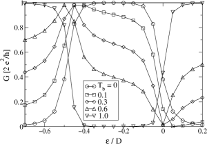
FIG. 2.: Linear-response conductance at zero temperature as a function of level position $\epsilon$ for different values of the background transmission $T_{\rm b}$. We have used $U/D=0.5$ and $\Gamma/D=0.063$, where the half bandwidth $D=1$ has been taken as the unit of energy. Note that due to the small ratio $\Gamma/D$, the results obtained here are cutoff–independent. The AB phase is $\varphi=0$.

The Kondo effect shows up at $T_{\rm b}=0$ as a large plateau of unitary transmission. At finite $T_{\rm b}$ the plateau survives but is reduced in height, similar to findings in recent experiments [6]. However, in these experiments the nature of the direct tunneling path has not yet been clarified. In particular, the direct tunneling strength cannot be tuned independently from the level broadening, which makes a quantitative comparison difficult. It would, therefore, be highly desireable to realize the geometry shown in Fig. 1 in order to directly verify the reduction of the Kondo plateau. This reduction, which we call the Fano-Kondo effect, can be understood analytically from Eq. (8). In the presence of interaction, the occupation of the dot is given by $\langle n\rangle\approx 1$ in the whole Coulomb blockade regime $-U+\bar{\Gamma}<\epsilon<-\bar{\Gamma}$, i.e., the resonant phase shift is $\delta_{\rm res}=\pi/2$, and Eq. (8) simplifies to

$$g_{\delta_{\rm res}=\pi/2}=\alpha\left(1-T_{\rm b}\cos^{2}\varphi\right)\,,$$ (9)

or $g=\alpha R_{\rm b}$ for $\varphi=0$ within the whole plateau. We emphasize that the Kondo effect does not break down. The reduction of the conductance plateau is rather due to interference between the lower (Kondo-) and the upper (reference) arm. For noninteracting systems, the phase is $\pi/2$ at resonance ($\epsilon=0$) only, i.e., there is no plateau. The formation of a reduced Fano-Kondo plateau is therefore a clear indication for Kondo correlations in the quantum dot under study. Far away from the plateau, we get $\delta_{\rm res}\rightarrow 0,\pi$, and thus $g=T_{\rm b}$ from Eq. (8) as expected. For arbitrary $\delta_{\rm res}$ we get

$$g_{\varphi=0}=\left[\alpha+(1-\alpha)T_{\rm b}\right]\sin^{2}(\delta_{\rm res}-\delta)\,.$$ (10)

This means that the conductance has a peak (of height $2e^{2}/h$ for $\alpha=1$ or $T_{\rm b}=1$) at $\delta_{\rm res}=\delta\pm\pi/2$ and is zero for $\delta_{\rm res}=\delta$ in agreement with Fig. 2. We emphasize the complementary behavior of the limiting cases of a closed ($T_{\rm b}=0$) and an open ($T_{\rm b}=1$) channel in the upper arm. For $T_{\rm b}=0$ we obtain the usual Kondo plateau [1, 3] but for $T_{\rm b}=1$ we have $\delta=\pi/2$ and the conductance is zero in the Kondo valley but $2e^{2}/h$ outside.

We now turn to the dependence of the conductance on the AB phase $\varphi$ and the question whether the phase $\delta_{\rm res}=\pi/2$ for unitary transmission in the Kondo regime can be detected from the AB oscillations of the linear conductance for a closed AB interferometer. We have calculated the shape of the AB oscillations for different gate voltages in and outside the Kondo regime, as shown in Fig. 3. Because of the phase locking property $G(\varphi)=G(-\varphi)$, we have plotted only $\varphi\in[0,\pi]$. The inset shows the lowest coefficients of the Fourier expansion $G(\varphi)=\sum_{n}\alpha_{n}\,e^{in\varphi}$.

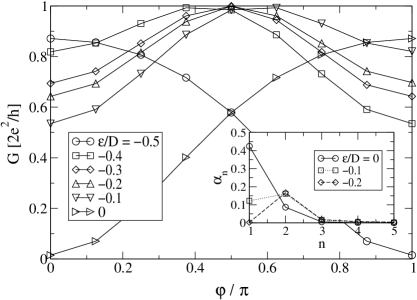
FIG. 3.: AB oscillations of the linear conductance for different level positions $\epsilon$. Parameters are identical to those in Fig. 2, with a background transmission of $T_{b}=0.3$. Inset: absolute value of Fourier coefficients, $|\alpha_{n}|$. In the Kondo regime, the first harmonic vanishes and $\alpha_{2}$ dominates, thus effectively doubling the frequency of the AB oscillations.

Outside the Kondo regime ($\epsilon/D=0$ and $-0.5$), the AB oscillations are dominated by the lowest harmonic (period $2\pi$), with global extrema at $\varphi=0,\pi$. A drastic change occurs as soon as the dot is tuned into the Kondo regime: then, the AB oscillations show a maximum at $\varphi=\pi/2$ with the universal conductance $2\alpha e^{2}/h$ independent of the value of the background transmission $T_{\rm b}$. As a consequence (see inset of Fig. 3), the $n=1$ Fourier coefficient vanishes, and the second harmonic dominates, thus effectively doubling the oscillation frequency. Due to Kondo screening, this frequency doubling persists over a finite range of gate voltages corresponding to the conductance plateau. This effect, therefore, yields a conveniently measurable and precise criterion for Kondo correlations in a quantum dot.

Figure 4 illustrates the “pinning” of the AB maximum. We show $G(\epsilon)$ for different AB phases $\varphi$. For $\varphi=\pi/2$ we recover a Kondo plateau with height

$$g_{\varphi=\pi/2}=\alpha+(T_{\rm b}-\alpha)\cos^{2}\delta_{\rm res}\,.$$ (11)

A special case is $T_{\rm b}=\alpha$ where the conductance is given by $2\alpha e^{2}/h$ for all level positions. Furthermore we note the property $G(\epsilon,\varphi)=G(-\epsilon-U,\varphi+\pi)$ which follows from particle-hole symmetry.

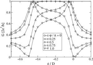
FIG. 4.: Dependence of the Fano lineshape on the AB phase for the same parameters as in Fig. 2 and a background transmission of $T_{\rm b}=0.3$.

Summary. We have studied the interplay of Kondo and Fano physics in the most basic model describing a closed AB interferometer which contains an interacting quantum dot in one of its arms. We derived a current formula and used Friedel sum rule to calculate the exact linear conductance at zero temperature with the help of the Numerical Renormalization Group generalized to two-channel systems. We found a characteristic Fano-suppressed Kondo plateau. Furthermore, we demonstrated that unitary transmission of a Kondo-correlated state can be identified by a frequency doubling of the AB oscillations and a conductance maximum at $\varphi=\pi/2$ with universal height.

Acknowledgements. We would like to thank Y. Gefen, D. Vollhardt, and W.G. van der Wiel for valuable discussions. This work is supported by the Deutsche Forschungsgemeinschaft under SFB 484 (W.H.) as well as under SFB 195 and the Emmy-Noether program (J.K.).

Note. While this paper was written up, a preprint [19] was published, in which a similar formula as Eq. (4) has been presented for the same model. However, we believe that the result of Ref. [19] is incorrect since it differs from our result by a factor $(1+x)$ in the second and third term.

REFERENCES

- [1] D. Goldhaber-Gordon et al., Nature 391, 156 (1998); S.M. Cronenwett et al., Science 281, 540 (1998); F. Simmel et al., Phys. Rev. Lett. 83, 804 (1999); J. Schmid et al., Phys. Rev. Lett. 84, 5824 (2000); W. G. van der Wiel et al., Science 289, 2105 (2000).
- [2] A.C. Hewson, The Kondo Problem to Heavy Fermions, (Cambridge University Press, 1993).
- [3] L.I. Glazman and M.E. Raikh, Sov. Phys. JETP Lett. 47, 452 (1988); T.K. Ng, P.A. Lee, Phys. Rev. Lett. 61, 1768 (1988); Y. Meir, N.S. Wingreen, and P.A. Lee, Phys. Rev. Lett. 70, 2601 (1993).
- [4] J. König, H. Schoeller, G. Schön, Phys. Rev. Lett. 76, 1715 (1996); J. König, J. Schmid, H. Schoeller, G. Schön, Phys. Rev. B 54, 16820 (1996)
- [5] A. Yacoby et al., Phys. Rev. Lett. 74, 4047 (1995); R. Schuster et al., Nature 385, 417 (1997); W.G. van der Wiel et al., Science 289, 2105 (2000); A.W. Holleitner et al., cond-mat/0011044.
- [6] J. Göres et al., Phys. Rev. B 62, 2188 (2000); I.G. Zacharia et al. cond-mat/0009140.
- [7] U. Fano, Phys. Rev. 124, 1866 (1961).
- [8] V. Madhavan et al., Science 280, 567 (1998).
- [9] O. Újsághy et al., Phys. Rev. Lett. 85, 2557 (2000).
- [10] M.A. Davidovich at al., Phys. Rev. B 55, R7335 (1997).
- [11] J. Friedel, Can. J. Phys. 34, 1190 (1956); D.C. Langreth, Phys. Rev. 150, 516 (1966).
- [12] M. Büttiker, Phys. Rev. B 46, 12485 (1992).
- [13] U. Gerland et al., Phys. Rev. Lett. 84, 3710 (2000); Y. Ji et al., Science 290, 779 (2000).
- [14] J. König and Y. Gefen, Phys. Rev. Lett. 86, 3855 (2001).
- [15] C. Bruder, R. Fazio, and H. Schoeller, Phys. Rev. Lett. 76, 114 (1996).
- [16] K.G. Wilson, Rev. Mod. Phys. 47, 773 (1975); T.A. Costi, A.C. Hewson, and V. Zlatić, J. Phys.: Cond. Mat. 6, 2519 (1994); W. Hofstetter, Phys. Rev. Lett. 85, 1508 (2000).
- [17] For vanishing AB phase the system can be mapped on an effective single-channel model by taking appropriate linear combinations of the reservoir degrees of freedom.
- [18] W. Hofstetter and S. Kehrein, Phys. Rev. B 59, R12732 (1999).
- [19] B.R. Bulka and P. Stefański, cond-mat/0104217; Phys. Rev. Lett. 86, 5128 (2001).