Scaling in a Nonconservative Earthquake Model of Self-Organised Criticality

Abstract

We numerically investigate the Olami-Feder-Christensen model for earthquakes in order to characterise its scaling behaviour. We show that ordinary finite size scaling in the model is violated due to global, system wide events. Nevertheless we find that subsystems of linear dimension small compared to the overall system size obey finite (subsystem) size scaling, with universal critical coefficients, for the earthquake events localised within the subsystem. We provide evidence, moreover, that large earthquakes responsible for breaking finite size scaling are initiated predominantly near the boundary.

PACS numbers: 05.65.+b, 45.70.Ht

I Introduction

Many dynamical phenomena in nature are intermittent. This “bursty” dynamics may be related to an underlying complex state, often characterised by long range correlations in space and time. For example, the crust of the earth alternates long periods of relative quiescence with burst of activity (earthquakes), which have a wide range of possible sizes. The behaviour of earthquakes is described by the empirical Gutenberg-Richter (GR) law [1], where the distribution of energy dissipated in earthquake events is a power law over many orders of magnitude in energy. The GR scaling extends from the smallest measurable earthquakes, which are equivalent to a truck passing by, to the most disastrous that have been recorded. Similar scale free behaviour of bursts is observed in vastly different kinds of physical systems such as flux motion through disordered type II superconductors placed in a magnetic field [2], or in granular piles, under some conditions [3], etc.

Self-organised criticality (SOC) [4] has been proposed as a general dynamical principal behind the observed complex behaviour of many natural phenomena. It refers to the fundamental property of slowly driven, extended systems to organise, over a sufficiently long transient period, into a dynamical critical state which lacks any characteristic time or length scale. The amplitude of the response of the system to an external perturbation follows a power law distribution. A number of simple models have been developed to test the applicability of SOC to a variety of complex interacting dynamical systems, such as sand piles and earthquakes (for a review see e.g. ref. [5, 6, 7]).

One of the basic theoretical problems is to identify robust, and thus physically relevant mechanisms for SOC to emerge, and to define a space of parameters and dynamical processes where SOC is a stable feature. Although it has been proposed that the presence of conservation laws (e.g. sand grains being transported in a sand pile) or special symmetries was necessary for SOC [8, 9], many known examples of physical phenomena and some models have been found where no apparent conservation law or special symmetry exists. These include, besides earthquakes, biological evolution, forest fires, epidemics, (possibly) solar flares, (possibly) reconnection events in the magnetotail, etc. [5, 6, 7]. In contrast to conservative systems, the mechanisms for SOC in non-conservative systems are not very well established.

A nonconservative SOC model that in recent years has attracted much attention is the so called OFC model [10]. The OFC model is a simplified lattice representation of a spring-block model for earthquake dynamics which was originally introduced by Burridge and Knopoff [11]. The Burridge-Knopoff model can be schematized as a two dimensional network of blocks interconnected by springs. All blocks are subject to an external driving force, which pulls them, and to a static friction, which opposes their motion. In the OFC model, each site of a lattice is associated with a continuous variable, which represent the force acting on a block. A slow driving is applied to the system by increasing uniformly and simultaneously the forces of all the elements. When the force on a site exceeds some threshold value (the maximal static friction), the site relaxes and distributes part of its force to nearest neighbour sites. Each such discharge event is accompanied by a local loss in accumulated force from the system. This conceptually simple and seemingly numerically tractable model reproduces some of the qualitative phenomenology of the statistics of earthquake events such as power law behaviour over a range of sizes, and intermittency or clustering of large events [12]. Extensions of the model have been recently developed which reproduce to some extent Omori’s law and other temporal patterns associated with earthquakes [13].

In the context of nonconservative models, the OFC model is of particular interest as it is possible to directly control the level of conservation of the dynamics through a parameter $\alpha$. Early analysis on relatively small systems indicated that the OFC model exhibited SOC, in the sense that earthquakes in the steady state obeyed finite size scaling (FSS) when the system size was varied [10]. However, the critical coefficients obtained using the FSS ansatz were found to be nonuniversal. In particular the exponents characterising the power law distributions appeared to vary with both the dissipation parameter, $\alpha$, and the form of the boundary conditions. This would have been in sharp contrast to the usual fixed point picture of critical phenomena where most microscopic details are irrelevant. Moreover some apparent critical exponents obtained using FSS violated physical bounds [14], putting some doubt on the existence of criticality in the model. Recently it was shown using a multiscaling analysis of large-scale simulations that, actually, the avalanche size distribution has a universal power law behaviour, independent of the dissipation parameter and for different boundary conditions, but that the cutoff in the power-law distribution does not behave according to FSS [15]. In larger systems, proportionally more of the force can be dissipated in the largest events that occur, and the cutoff function becomes sharper and sharper as the system size increases.

Departures from standard FSS have been reported for various SOC models as, for example, the sandpile model [16], the Drossel-Schwabl (DS) forest fire model [17, 18] and the Zhang model [19]. In this paper we address the question of the origin of the breaking of FSS and its relation to the mechanism responsible for SOC in the OFC model. In particular we test the implicit assumption behind the FSS hypothesis that a finite systems behaves as a subsystem of a larger system. The paper is organised as follows. In the section II we describe in some detail the model. In section III we present the results of our numerical study relative to two different type of probability distributions for earthquake sizes. The first distribution concerns earthquakes which are localised within a given subsystem. We show that this subset of earthquakes exhibits ordinary FSS as long as the linear extent, $\lambda$, of the subsystem is sufficiently small compared to the linear extent, $L$, of the entire system. The second distribution groups earthquakes according to the position of their starting site relative to the boundaries of the system. From this investigation, we deduce that FSS is violated due to large events initiated in a region near the boundary. Finally, in section IV we discuss our results and draw some conclusions.

II The model

We consider a two-dimensional square lattice of $L\times L$ sites. To each site $i$ of the lattice we associate a continuous variable $F_{i}$, which initially take some random values between zero and a threshold value $F_{th}$. The dynamics proceeds then indefinitely. In the limit of infinite time scale separation between the slow driving and the (almost) instantaneous earthquake process, the dynamics is:

1. Uniform drive: all forces $F_{i}$ are increased at the same rate, until one of them reaches the value $F_{th}$.

2. Earthquake: when a site becomes unstable (i.e $F_{i}\geq F_{th}$), the uniform driving is stopped and the system evolves according to the following local relaxation rule

   $$F_{i}\geq F_{th}\Rightarrow\left\{\begin{array}[]{l}F_{i}\rightarrow 0\\ F_{nn}\rightarrow F_{nn}+\alpha F_{i}\end{array}\right.$$ (1)

   until there are no more unstable sites. In eq. (1), the subscript “nn” stands for the four nearest neighbours to site $i$.

Since only a fraction, $4\alpha$, of the force is redistributed in each relaxation event (toppling), the model is nonconservative for $\alpha<1/4$. In the following we concentrate on this case, i.e. $0<\alpha<1/4$.

To completely define the model we need to specify the boundary conditions. Boundaries are believed to play a crucial role for the observation of critical behaviour in the OFC model. It has been suggested that they act as inhomogeneities which frustrate the natural tendency of the model to order into a periodic state [20, 21]. Indeed, for sufficiently small values of the conservation parameter $\alpha$ ($\alpha<\alpha_{c}\simeq 0.18$), a system with periodic boundary conditions quickly reaches an exactly periodic state with only earthquakes of size one. For larger values of $\alpha$ the situation is slightly more complicated with multiple topplings involved in a single avalanche, but the avalanches are still localised and criticality is not observed [20]. A system with open boundaries is prevented from reaching a periodic state because boundary sites have fewer neighbours and therefore cycle at a different frequency from bulk sites. Middleton and Tang suggested that the inhomogeneity created by the boundaries propagates into the bulk of the system, developing, in this way, long range spatial correlations. They named this mechanism “marginal synchronisation” or phase locking [22]. In accordance with previous studies, therefore, we consider open boundary conditions. If a boundary (corner) site topples, an extra amount $\alpha F_{i}$ ($2\alpha F_{i}$) is simply lost by the system.

III Results: probability distributions

After a sufficiently long transient time, the system reaches a stationary state. Several statistical properties can be used to characterise this state. Most previous studies of the OFC model have focused on the behaviour of the probability distribution of earthquake sizes, $P_{L}(s)$, where $L$ is the size of the system and $s$ is the total number of topplings events during an earthquake [10, 15, 20, 21, 22, 23, 24, 25]. We choose instead to analyse the behaviour of different distributions for avalanches sizes, which distinguish between earthquakes according to the region of the lattice involved (e.g. bulk or boundary) and the coordinates of the triggering site (see figure 1). This investigation is particularly relevant for the OFC model in view of the strong inhomogeneity in the spatial distribution of avalanches [20, 22, 25]. According to ref. [20], for example, large avalanches are localised near the boundary (at least for $\alpha<\alpha_{c}$). As a minor technical remark, we point out that we exclude from our data avalanches which involve only one site ($s=1$) as they appear to behave according to their own statistics [20]. As we are mainly interested in asymptotically large earthquakes, this does not alter our conclusions.

We consider a subsystem of linear extent $\lambda$ centred in a system of size $L$. The first distribution we introduce, $P_{conf}(\lambda,L,s)$, is the normalised distribution of earthquake sizes restricted to earthquakes which are confined entirely within the subsystem (e.g. avalanche (a) in fig. 1). The model is driven according to its usual dynamics but only those particular earthquakes are counted. According to our definition, the case $\lambda=L$ corresponds to the distribution of avalanches which do not reach the boundary of the system. As shown in fig. 2, the distribution $P_{conf}(\lambda,L,s)$ becomes independent of $L$, if $L$ is considerably larger then $\lambda$ (approximately $L\geq 2\lambda$). When $L$ approaches $\lambda$, this is no longer the case and the cutoff in the distribution is pushed to larger sizes. Although we have shown in Fig. 2 only the distributions for $\alpha=0.18$ and $\lambda=32,64$, analogous considerations apply to different values of $\alpha$ and for different sizes, $\lambda$. Since for a generic $L$, $P_{conf}(\lambda,L,s)\neq P_{conf}(\lambda,\lambda,s)$, a small portion of a large system is substantially different from a finite system of the same size, contrary to what happens in equilibrium critical phenomena. A similar observation was made in ref. [17] for the DS forest fire model. In the following, we denote with $P_{conf}(\lambda,s)$ the distribution $P_{conf}(\lambda,L,s)$ in the limit where the distribution does not appear to depend on $L$. In order to determine numerically these distributions, for each value of $\lambda$ we have simulated (for at least $2\cdot 10^{9}$ earthquakes) a system of size $L=2\lambda$. The dependence on $L$ of $P_{conf}$ can in this case be safely neglected. With this choice, the accuracy of the measures and the range of scales investigated are optimised, within our computational limits.

In Fig. 3 we report a FSS collapse of $P_{conf}(\lambda,s)$ for different values of $\alpha$ . Contrary to the entire distribution of earthquake sizes, $P_{L}(s)$, we observe that $P_{conf}(\lambda,s)$ satisfies the FSS hypothesis, i.e. $P_{conf}(\lambda,s)\simeq\lambda^{-\beta}f(s/\lambda^{D})$, with universal critical coefficients. The curve corresponding to $\alpha=0.15$ and $\lambda=256$ shows some noisy behaviour, due to the difficulties in collecting good statistics in this case. Indeed by decreasing $\alpha$, the relative fraction of earthquakes in the bulk of the system (with size $s>1$) diminishes. Nonetheless, there is no evident sign that FSS is violated in this case. The critical exponents used in the fit of Fig. 3 are $\beta=3.6$ and $D=2$, independent of the dissipation parameter $\alpha$. The value of the histogram exponent $\tau=\beta/D\simeq 1.8$ we obtain is the same as that found for $P_{L}(s)$ [15]. In addition, the value of $D$ we find corresponds to the largest possible value for the entire distribution ($D_{max}$ in ref. [15]), as it can be shown that non-conservation requires $D\leq 2$ [14].

The scaling behaviour of $P_{conf}$ appear to be reasonably robust with respect to translating the subsystem within the entire system; in fig. 4 we report a FSS plot for the subsystem placed on a boundary and on a corner of the system for $\alpha=0.18$. While the FSS collapse for the subsystem placed on the boundary is rather good, some deviations from FSS are observed in the cut-off region for the case of the subsystem placed in the corner. We believe this behaviour can be ascribed to the enhanced boundary effects in the latter case (two side of the subsystem are boundary sides instead of only one) and would disappear if larger (sub)systems could be studied. This picture is confirmed by choosing different $\alpha$ values: for the subsystem in the corner, deviations from FSS are more pronounced for $\alpha=0.21$ and are absent for $\alpha=0.15$. For the subsystem on the boundary, instead, the quality of FSS collapse is rather convincing in all cases.

We introduce next the distributions $P_{<}(\lambda,L,s)$ and $P_{>}(\lambda,L,s)$. These are the normalised distribution of earthquakes which start respectively within ($P_{<}$) and outside ($P_{>}$) the subsystem of size $\lambda$, irrespective of whether they stay in or go out of the subsystem (see fig. 1). The only difference between these two distributions, $P_{<}$ and $P_{>}$, is the location of the site that triggers the avalanche. We observe numerically that the distributions $P_{<}(\lambda,L,s)$ and $P_{>}(\lambda,L,s)$ become independent of $\lambda$ respectively in the limit $\lambda\ll L$ and $\lambda\simeq L$. As an example we report in Fig. 5 the behaviour of $P_{<}(\lambda,L,s)$ and $P_{>}(\lambda,L,s)$ for $\alpha=0.18$, $L=256$ and for various $\lambda$. For simplicity, in the following we denote with $P_{<}(L,s)$ and $P_{>}(L,s)$ the distributions in the limit where they do not depend on $\lambda$.

We consider therefore two centred subsystems of linear extent $\lambda_{2}>\lambda_{1}$, such that the above conditions are satisfied. More specifically, we choose $\lambda_{1}=\frac{3}{16}L$ and $\lambda_{2}=\frac{7}{8}L$. In this case $P_{>}$ corresponds to the subset of earthquakes which are initiated in some “boundary” region and $P_{<}$ corresponds to the subset of earthquakes which are initiated within some “bulk” region. In fig. 6 we report a FSS scaling plot both for $P_{>}$ and $P_{<}$. In this figure we choose $D=2$ as the maximum allowed value. It is clear that the boundary distribution $P_{>}$ cannot be collapsed according to the FSS ansatz. In fact it develops a sharper and sharper cutoff which changes shape and which has an excess of large events (the cutoff moves towards right for increasing $L$). The bulk distribution $P_{<}$ instead does not develop a noticeably sharper cutoff and does not appear to change its shape. It may possibly be collapsed according to the FSS ansatz. Consistent with the results for $P_{conf}$ and for $P_{L}$, the power law exponent for $P_{<}$ is $\tau=\beta_{1}/D\simeq 1.8$.

The above numerical analysis indicates that the large events which violate FSS are triggered by sites in a boundary region. Indeed the behaviour of the cutoff for the collapsed probability distributions $P_{>}$ and $P_{L}$ is very similar (see Fig. 1 in ref. [15]). Although large earthquakes are focussed mainly toward the boundary, as suggested in ref. [20], they occur also in the bulk of the system, even for low values of $\alpha$, as can be deduced from Fig. 3 and Fig. 6. Moreover, we do not observe any significant qualitative change in the behaviour of the system around $\alpha=\alpha_{c}\simeq 0.18$, as claimed in ref. [20].

IV Discussion and conclusions

Similarly to other SOC systems [16, 17, 18, 19], the nonconservative OFC model shows relevant deviations from simple FSS [15]. In this paper we have investigated the origin of this phenomenon, finding that FSS in the OFC model is violated because of large, system wide earthquakes. In fact, we have found that earthquakes localised within a given subsystem do obey ordinary FSS, with universal critical exponents, independently of whether the subsystem is placed at the centre or on a boundary of the system. The value of the power law exponent, $\tau\simeq 1.8$, for the “confined” distribution agrees with the one for the entire distribution. We have shown, moreover, that the probability distribution for earthquakes initiated in a boundary region do not obey FSS, because of an “excess” of large events. This would result in an apparent exponent $D>2$ which is not allowed in the nonconservative case. On the other hand, the probability distribution for earthquakes starting in the bulk of the system is compatible with a FSS hypothesis. In particular, the critical exponent is $D=2$ in this case, indicating that large earthquakes responsible for breaking finite size scaling are initiated predominantly near the boundary of the system.

Self-organised criticality in the OFC model has been ascribed to a mechanism of “marginal synchronisation” [22]. A system with open boundaries becomes almost synchronised by an invasion process where spatial correlations develop from the boundaries. It was suggested that sites close to the boundaries start to organise themselves first, building up long range correlations. The critical region grows with time, until, in the stationary state, it invades the whole lattice . Our findings on the large events occurring at the boundary seem to indicate that the effect of synchronisation is stronger for boundary sites than for bulk sites. This view is supported also by the “on screen” observation that large earthquakes tend to be triggered repetitively by the same sites over a long time scale (a result which seems to be confirmed also by the study in ref. [25]).

S.L. acknowledges financial support from EPSRC (UK), Grant No. GR/M10823/01.

FIG. 1.: Schematic representation of different types of avalanches. The continuous line represents the lattice of size $L$, the dashed line the subsystem of linear extent $\lambda$. Triggering sites are denoted with a full circle, toppling sites with a cross. Avalanche (a) contributes to the distribution $P_{conf}(\lambda,L,s)$; (a) and (b) to $P_{<}(\lambda,L,s)$; (c) to $P_{>}(\lambda,L,s)$.

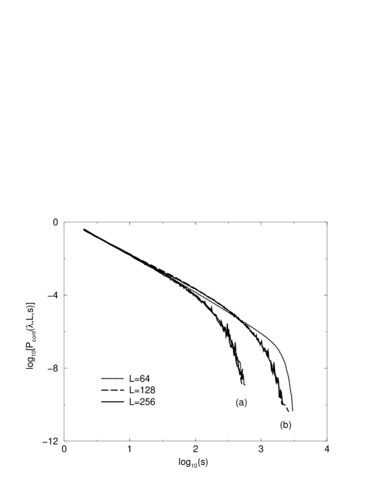
FIG. 2.: Probability distribution $P_{conf}(\lambda,L,s)$ for $\alpha=0.18$ and (a) $\lambda=32$ and (b) $\lambda=64$.

FIG. 3.: Finite-size scaling plots of $P_{conf}(\lambda,s)$ (with the subsystem placed at the centre) for (a) $\alpha=0.15$, (b) $\alpha=0.18$ and (c) $\alpha=0.21$. The critical exponents are $\beta=3.6$ and $D=2$; the slope of the straight line is $\tau=1.8$. For visual clarity, curves (a) and (c) have been shifted along the $x$-axis, $x\rightarrow x-1$ and $x\rightarrow x+1$ respectively.

FIG. 4.: Finite-size scaling plots of $P_{conf}$ for the subsystem placed (a) on a corner and (b) on a boundary of the system ($\alpha=0.18$). The critical exponents are $\beta=3.6$ and $D=2$; the slope of the straight line is $\tau=1.8$. Curve (a) has been shifted, $x\rightarrow x-1$.

FIG. 5.: Probability distributions (a) $P_{<}(\lambda,L,s)$ and (b) $P_{>}(\lambda,L,s)$ for $\alpha=0.18$, for $L=256$ and for various $\lambda$.

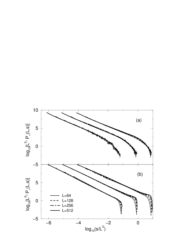
FIG. 6.: Finite-size scaling plots of (a) $P_{<}(L,s)$ and (b) $P_{>}(L,s)$. Different sets of curves corresponds, from left to right, to $\alpha=0.15$ (shifted by $x\rightarrow x-1$), $\alpha=0.18$ and $\alpha=0.21$ (shifted by $x\rightarrow x+1$). The exponents are $\beta_{1}=3.6$, $\beta_{2}=3.9$ and $D=2$.

REFERENCES

- [1] B. Gutenberg and C.F. Richter, Ann. Geofis. 9, 1 (1956).
- [2] S. Field, J. Witt, F. Nori and X.S. Ling, Phys. Rev. Lett. 74, 1206 (1995); C. Heiden and G.I. Rochlin, Phys. Rev. Lett. 21, 691 (1968).
- [3] V. Frette, et. al., Nature 379, 49 (1996).
- [4] P. Bak, C. Tang, and K. Wiesenfeld, Phys. Rev. Lett. 59, 381 (1987); Phys. Rev. A. 38, 364 (1988).
- [5] P. Bak, How Nature Works: The Science of Self-Organized Criticality (Copernicus, New York, 1996).
- [6] H. Jensen, Self-Organized Criticality (Cambridge University Press,New York, 1998).
- [7] D. L. Turcotte, Rep. Prog. Phys. 62 (10) 1377 (1999).
- [8] T. Hwa and M. Kardar, Phys. Rev. Lett. 62, 1813 (1989).
- [9] G. Grinstein, D.-H. Lee, and S. Sachdev, Phys. Rev. Lett. 64, 1927 (1990).
- [10] Z. Olami, H.J.S. Feder, and K. Christensen, Phys. Rev. Lett. 68, 1244 (1992); K. Christensen and Z. Olami, Phys. Rev. A 46, 1829 (1992).
- [11] R. Burridge and L. Knopoff, Bull. Seismol. Soc. Am. 57,341 (1967).
- [12] K. Christensen and Z. Olami, J. Geophys. Res. 97, 8729 (1992); K. Christensen, Z. Olami, and P. Bak, Phys. Rev. Lett. 68, 2417 (1992).
- [13] S. Hainzl, G. Zoller, and J. Kurths, J. Geophys. Res. 104, 7243 (1999); Nonlinear Proc. Geoph. 7, 21 (2000).
- [14] W. Klein and J. Rundle, Phys. Rev. Lett. 71, 1288 (1993).
- [15] S. Lise and M.Paczuski, Phys. Rev. E, 63, 036111 (2001).
- [16] M. De Menech, A. L. Stella, and C. Tebaldi, Phys. Rev. E 58, 2677 (1998); C. Tebaldi, M. De Menech, and A. L. Stella, Phys. Rev. Lett. 83, 3952 (1999).
- [17] K. Schenk, B. Drossel, S. Clar, and F. Schwabl, Eur. Phys. J. B 15, 177 (2000)
- [18] R. Pastor-Satorras and A. Vespignani, Phys. Rev. E 61, 4854 (2000)
- [19] R. Pastor-Satorras and A. Vespignani, Eur. Phys. J. B 18, 197 (2000)
- [20] P. Grassberger, Phys. Rev. E 49, 2436 (1994).
- [21] J.E.S. Socolar, G. Grinstein, and C. Jayaprakash, Phys. Rev E, 47, 2366 (1993).
- [22] A. A. Middleton and C. Tang, Phys. Rev. Lett. 74, 742 (1995).
- [23] I.M. Jánosi and J. Kerteśz, Physica A 200, 174 (1993).
- [24] Á. Corral, C. J. Pérez, A. Díaz-Guilera, and A. Arenas, Phys. Rev. Lett. 74, 118 (1995).
- [25] H. Ceva, Phys. Lett. A, 245, 413 (1998).