Simulations of the Static Friction Due to Adsorbed Molecules

Abstract

The static friction between crystalline surfaces separated by a molecularly thin layer of adsorbed molecules is calculated using molecular dynamics simulations. These molecules naturally lead to a finite static friction that is consistent with macroscopic friction laws. Crystalline alignment, sliding direction, and the number of adsorbed molecules are not controlled in most experiments and are shown to have little effect on the friction. Temperature, molecular geometry and interaction potentials can have larger effects on friction. The observed trends in friction can be understood in terms of a simple hard sphere model.

I Introduction

The last decade has seen great advances in techniques for measuring friction in contacts whose geometry and/or chemistry are controlled with atomic precision.[1, 2, 3, 4, 5, 6] At the same time, increases in computational power have allowed increasingly realistic simulations of friction.[7, 8] These studies reveal unexpected behavior that raises questions about the molecular origins of static friction and the “laws” of friction that describe most macroscopic objects.

Friction is the lateral force needed to slide one object over another. The force needed to initiate sliding is called the static friction $F_{\rm s}$. Its existence implies that the surfaces have locked into a local free energy minimum, and $F_{\rm s}$ represents the lateral force needed to displace them out of this minimum. The force needed to maintain a constant sliding velocity $v$ is called the kinetic friction $F_{k}(v)$, and it represents the force required to replace energy dissipated during sliding.

Macroscopic objects almost always exhibit a finite static friction and a kinetic friction that is slightly smaller at low velocities. One puzzling result from many molecular scale theories of friction between bare surfaces is that the static friction almost always vanishes, and is not closely related to the kinetic friction.[7, 9] This indicates that some important feature is missing from these model systems, that must be included to make contact with macroscopic experiments. Of course real surfaces are generally not bare, but are coated with a layer of adsorbed molecules, as well as dust, dirt and other debris. In this paper we explore the influence of a layer of molecules between two surfaces on friction forces, and show that including such layers naturally leads to behavior that is consistent with macroscopic measurements.

Over three hundred years ago Amontons’ published two “laws” of macroscopic friction that are still taught and used today.[10] These state that the friction is proportional to the normal load $L$ pushing two surfaces together, and independent of the apparent geometrical area of these surfaces $A_{\rm app}$. Subsequent work [3, 4, 11, 12, 13, 14, 15, 16] is consistent with a more general friction formula that is based on the observation[17, 18, 19] that the actual area of molecular contact between two surfaces $A_{\rm real}$ is much smaller than the nominal surface area $A_{\rm app}$. The friction is assumed to be given by $A_{\rm real}$ times a local shear stress $\tau$. If $\tau$ rises linearly with the local contact pressure $P$,

$$\tau=\tau_{0}+\alpha P\ \ \ ,$$ (1)

then since $P=L/A_{\rm real}$

$$F=\tau A_{\rm real}=\tau_{0}A_{\rm real}+\alpha L\ \ \ .$$ (2)

This expression agrees with Amontons’ laws if $A_{\rm real}$ is proportional to $L$ or if $\tau_{0}$ is sufficiently small compared to $\alpha P$. The former condition applies if the load is high enough to produce plastic deformation of the surfaces so that $L/A_{\rm real}$ remains equal to the hardness.[17] It also holds for non-adhesive contacts between ideal elastic solids with random surface roughness.[20, 21] However, any adhesive bonding leads to friction in the limit of zero load and violates Amontons’ laws. For a piece of adhesive tape the first term in Equation 2 dominates at low loads, and in many cases friction can be observed at negative loads.

Early attempts to explain Amontons’ laws and the existence of static friction were based on the idea that peaks on one surface interlock with valleys on the other surface.[10, 17] In order to slide, the top surface must then be lifted up a ramp formed by the typical slope $\tan\psi$ of the bottom surface. If there is no microscopic friction between the surfaces, then the minimum lateral force to initiate sliding is $F_{\rm s}=L\tan\psi$. This result satisfies Amontons’ laws with a constant coefficient of friction $\mu_{\rm s}\equiv F_{\rm s}/L=\tan\psi$ that can span all possible values. However, this geometrical model for friction can not explain many experimental observations. For example, coating a single monolayer of surfactant on a surface does not change its slope, but can reduce the friction by more than an order of magnitude. It is also well known that making surfaces too smooth actually leads to an increase in friction.[17, 22] A practical illustration of this is that magnetic hard disks are purposely roughened to reduce friction.

The fundamental problem with the above explanation for the origin of static friction is that there is no reason for the peaks from different surfaces to be correlated. In general one expects that at any instant in time some peaks will be moving up a ramp and an equal number of peaks will be moving down. The net lateral force will average to zero and there will be no static friction. A similar problem arises if one imagines that the interlocking peaks are individual atoms as in the “cobblestone” model discussed by Israelachvili and coworkers.[15, 23] If atoms are from two identical, aligned surfaces all of them will go up ramps simultaneously yielding Amontons’ laws. However, friction measurements are usually made between misaligned surfaces or surfaces with different lattice constants. In this case the force from atoms moving up ramps should cancel the force from atoms moving downward, yielding a vanishing static friction.

A number of detailed analytic[24, 25, 26, 27, 28] and simulation [7, 29, 30, 31, 32, 33, 34] studies have concluded that $F_{\rm s}$ should generally vanish between bare crystalline or disordered surfaces. The exception is the case of commensurate surfaces which share a common periodicity in their plane of contact. In this case the free energy varies with the phase difference between the common Fourier components, and simulations of such surfaces[35, 36] find a static friction that rises linearly with pressure as in Eq. 1. However the probability that two contacting surfaces are commensurate is infinitesimally small. Even identical surfaces are only commensurate when they are perfectly aligned.[29] Any misorientation (Figure 1) causes the surfaces to become incommensurate, i.e. have no common period. The free energy is then independent of translations and $F_{\rm s}$ is identically zero.[25, 26, 28] If the interactions between the two surfaces are strong enough compared to interactions within the surfaces they may deform into a commensurate structure.[25, 26, 34] However, this criterion is unlikely to be met for most of the surfaces around us, which have been chemically passivated by exposure to air. Indeed calculations for clean surfaces in vacuum find zero static friction between different facets of the same metal![28, 29, 32, 37] Moreover, contacts that are known to be in the elastic limit exhibit static friction.[3, 4, 14, 15, 16] Edge effects can lead to a finite static friction, but are not significant for the micron size contacts typically found between macroscopic objects.[38] Chemical disorder and surface roughness are also unable to produce observed friction forces.[21, 38, 39, 40]

There are relatively few direct experimental measurements of the friction between bare crystalline surfaces. However, studies of adsorbed monolayers,[41, 42] small crystalline tips,[43] mica,[44] and molybdenum disulphide[45] support the conclusion that friction vanishes in this limit. A finite friction has been observed between clean metallic surfaces,[17, 46] but the surfaces were rough and the load appears to have been high enough to produce plastic deformation. Further work in this area would be of great value in testing the above theoretical models.

In recent papers[34, 38, 47, 48] we have suggested that the so-called “third bodies” that are present between most contacting surfaces[49, 50] can provide a general mechanism for static friction. These third bodies may take the form of wear debris, dust, or small hydrocarbon or water molecules that are adsorbed from the air. The interactions between such bodies are generally weaker than the interactions within the bounding solids. This frees them to rearrange at the interface to lower their free energy and lock the surfaces together. The layer of third bodies creates an immense number of metastable states, like that in a glass or granular medium. The third bodies can always fall into one of these states that is in registry with both bounding walls and thus produce static friction.[51]

In this paper we report extensive studies of the static friction produced by layers of spherical or short chain molecules between crystalline surfaces. We begin by describing different methods of measuring the static friction and establishing that it has a well-defined thermodynamic limit. Then the effect of temperature, wall geometry, interaction potentials, chain length and areal density on the static friction are explored. In each case the static friction obeys Equation 1 over the experimentally relevant pressure range. Factors that are not controlled in typical macroscopic experiments have little influence on $\tau_{0}$ and even less effect on $\alpha$, which dominates the friction at high loads. Such factors include wall geometry, sliding direction, and the length and density of adsorbed molecules. Increasing the temperature lowers $\tau_{0}$, but has relatively little effect on $\alpha$. The value of $\alpha$ is strongly dependent on the interaction potential, particularly the effective hard sphere size of the molecules compared to that of wall atoms. All of our results can be understood in terms of a simple geometrical explanation for the origin of Equation 1.

The following section describes the details of our simulations and the algorithms used to determine $F_{\rm s}$. Section III determines the effect of each parameter in our simulations on the static friction and describes a simple geometrical picture that explains all of the observed trends. The final section summarizes the results.

II Simulation Method

A Potentials and geometry

We use a bead spring model[52] that allows us to explore the behavior of simple spherical molecules or short chains between bounding solids. Each molecule contains $n$ spherical monomers. All monomers interact with each other through a truncated Lennard-Jones potential:

$$V(r)=\left\{\begin{array}[]{ll}4\epsilon[(\sigma/r)^{12}-(\sigma/r)^{6}-(\sigma/r_{\rm c})^{12}+(\sigma/r_{\rm c})^{6}]&;r<r_{\rm c}\\ 0&;r>r_{\rm c}\ \ \ \ \ .\end{array}\right.$$ (3)

The parameters $\sigma$ and $\epsilon$ are chosen as the units of length and energy, respectively. Combined with the monomer mass $m$, they determine the unit of time $t_{\rm LJ}=(m\sigma^{2}/\epsilon)^{1/2}$. Typical values for hydrocarbons are: $\sigma\sim 0.5$nm, $\epsilon\sim 30$meV and $t_{\rm LJ}\sim 3$ps. We consider the case $r_{\rm c}=2^{1/6}\sigma$ to simulate a purely repulsive potential, and $r_{\rm c}=2.2\sigma$ is used to study the effect of adhesive forces.

Monomers are bound into chains by an additional strongly attractive potential between nearest neighbors on the same molecule:

$$V^{\rm CH}(r)=\left\{\begin{array}[]{ll}-\frac{1}{2}kR_{0}{\rm ln}[1-(r/R_{0})^{2}],&r<R_{0}\\ \infty&r\geq R_{0}\end{array}\right.$$ (4)

where $R_{0}=1.5\sigma$ and $k=30\epsilon\sigma^{-2}$. These parameters are chosen to prevent chain crossing as described in previous work.[52] We consider the case of spherical molecules ($n=1$), and of short chains with $n=3$ and $6$. Based on mappings of the bead-spring model to real molecules,[52] this corresponds to alkane chains with up to roughly 16 carbons. Substantially longer molecules are unlikely to have sufficient volatility to contribute to the airborn contamination that is present on any surface. Polymers are often placed at interfaces intentionally to act as lubricants. We have not addressed the behavior of these much longer molecules.

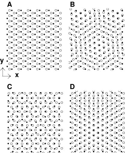
FIG. 1.: Projections into the $x-y$ plane of atoms from the inner surfaces of the bottom (solid circles) and top (open circles) walls. In A through C the two walls have the same structure and lattice constant, but the top wall has been rotated by $0^{\circ}$, $8.2^{\circ}$, or $90^{\circ}$, respectively. In D the walls are aligned, but the lattice constant of the top wall has been reduced by 12/13. The atoms can only achieve perfect registry in the commensurate case A. The simulation cell was usually at least four times the area shown here.

Molecules are confined between two walls formed by the (111) surfaces of fcc crystals directed normal to the $z$-axis. Wall atoms are connected to their lattice sites with springs of stiffness $k_{\rm s}$ in order to model elastic deformation in the simplest way.[53] We consider the completely rigid case, $k_{\rm s}=\infty$, and $k_{\rm s}=840\epsilon/\sigma^{2}$ or $210\epsilon/\sigma^{2}$. Both of the latter values correspond to relatively compliant solids. For example, at $T=0.8\epsilon/k_{B}$ they lead to root mean squared (rms) displacements about lattice sites that are about 4.5 and 9%, respectively, of the nearest neighbor separation (1.2$\sigma$) used in most of our simulations.[54]

Wall atoms and fluid monomers also interact with a Lennard-Jones potential but with different characteristic energy and length scales $\sigma_{\rm wf}$ and $\epsilon_{\rm wf}$, respectively. These are varied to determine the effect of molecular size and chemistry on static friction. Direct interactions between atoms on different walls are not included in the simulations. They vanish identically for the short cutoff $r_{\rm c}=2^{1/6}\sigma$ used in most of our simulations, and have a very small effect on calculated quantities at larger $r_{\rm c}$. Tests of the effect of wall-wall interactions are discussed briefly in Section III F.

Periodic boundary conditions are imposed in the plane of the walls. These periodic boundary conditions prevent us from considering truly incommensurate systems. However, the effect of commensurability rapidly decreases as the length of the common period increases.[7, 34, 38, 55] The degree of commensurability between the walls is varied in two ways. The first is to rotate the top wall by an angle $\theta$ about the $z$-axis (Fig. 1 A-C). Only the range of $\theta$ from 0 to 30^∘ produces inequivalent results. The second is to retain the alignment of the two lattices ($\theta=0$), but to change the ratio of the lattice constants of the bottom and top walls from unity to $12/13$ (Fig. 1 D).

TABLE I.: Values of the orientation angle $\theta$ and the corresponding two dimensional basis vectors and number of atoms per surface layer in the top wall. Both surfaces have hexagonal symmetry. The final column gives the percentage difference between the nearest-neighbor spacings in the two walls.

$\theta$	$\vec{b_{1}}/d$	$\vec{b_{2}}/d$	No. of atoms	$\frac{d-d^{\prime}}{d}$ ($\%$)
$0^{\circ}$	$\vec{i}$	$\frac{1}{2}\vec{i}+\frac{\sqrt{3}}{2}\vec{j}$	$2304$	0
$2.02^{\circ}$	$\frac{588}{601}\vec{i}+\frac{12\sqrt{3}}{601}\vec{j}$	$\frac{276}{601}\vec{i}+\frac{300\sqrt{3}}{601}\vec{j}$	$2404$	$-2.1$
$4.127^{\circ}$	$\frac{192}{193}\vec{i}+\frac{8\sqrt{3}}{193}\vec{j}$	$\frac{84}{193}\vec{i}+\frac{100\sqrt{3}}{193}\vec{j}$	$2316$	$-0.3$
$6.3^{\circ}$	$\frac{564}{559}\vec{i}+\frac{36\sqrt{3}}{559}\vec{j}$	$\frac{228}{559}\vec{i}+\frac{300\sqrt{3}}{599}\vec{j}$	$2236$	$1.5$
$8.2^{\circ}$	$\frac{48}{49}\vec{i}+\frac{4\sqrt{3}}{49}\vec{j}$	$\frac{18}{49}\vec{i}+\frac{26\sqrt{3}}{49}\vec{j}$	$2352$	$-1.03$
$10.4^{\circ}$	$\frac{564}{571}\vec{i}+\frac{60\sqrt{3}}{571}\vec{j}$	$\frac{192}{571}\vec{i}+\frac{312\sqrt{3}}{571}\vec{j}$	$2284$	$0.44$
$14.4^{\circ}$	$\frac{564}{589}\vec{i}+\frac{84\sqrt{3}}{589}\vec{j}$	$\frac{156}{589}\vec{i}+\frac{324\sqrt{3}}{589}\vec{j}$	$2356$	$-1.1$
$19.1^{\circ}$	$\frac{20}{21}\vec{i}+\frac{4\sqrt{3}}{21}\vec{j}$	$\frac{4}{21}\vec{i}+\frac{12\sqrt{3}}{21}\vec{j}$	$2268$	$0.79$
$25.2^{\circ}$	$\frac{33}{37}\vec{i}+\frac{9\sqrt{3}}{37}\vec{j}$	$\frac{3}{37}\vec{i}+\frac{21\sqrt{3}}{37}\vec{j}$	$2368$	$-1.4$
$30^{\circ}$/$90^{\circ}$	$\frac{6}{7}\vec{i}+\frac{2\sqrt{3}}{7}\vec{j}$	$\frac{4\sqrt{3}}{7}\vec{j}$	$2352$	$-1.03$

The simulation cell is a rectangle whose height along $y$ is $\sqrt{3}/2$ times the length along $x$, and the [110] direction of the bottom wall is directed along the $x$ axis. Special values of $\theta$ are chosen that allow both top and bottom surfaces to retain perfect triangular symmetry, and to have nearly the same nearest-neighbor spacings. Values for the percentage difference between the spacing on the bottom, $d$, and on the top, $d^{\prime}$, walls are given in Table I. The difference is typically less than $2\%$, and no trends were seen with the sign or magnitude of this difference.

The system is thermostatted by coupling to a heat reservoir through Langevin noise and damping terms in the equation of motion.[56] Previous work shows that coupling along the direction of sliding produces a direct effect on the kinetic friction, while coupling to the perpendicular components does not.[7, 33, 57] Thus only the perpendicular components are thermostatted, using the equation of motion:

$$m\ddot{\vec{x}}_{\perp}=\vec{F_{\perp}}-m\Gamma\dot{\vec{x}}_{\perp}+\vec{W}_{\perp}\ \ \ .$$ (5)

Here $F$ is the force from the interaction potentials, $\Gamma$ is the friction constant that controls the rate of heat exchange with the reservoir, and $W$ is the Gaussian-distributed random force acting on each monomer. The rms value of $W$ is determined from $\Gamma$ through the usual fluctuation-dissipation relation.[56] The equations of motion are integrated using a fifth-order, Gear predictor-corrector algorithm.[58] In most cases the time step $dt=0.005t_{\rm LJ}$ and $\Gamma=0.4t_{\rm LJ}^{-1}$. As discussed in Sec. III A, our measured static friction forces are insensitive to the choice of $\Gamma$.

The areal density of monomers is specified as the effective coverage on the separate surfaces before they are brought into contact. To avoid ambiguities in the definition of the monolayer density, we define the coverage as the number of adsorbed monomers divided by the total number of wall atoms in the surface layers of both walls. A coverage of 1/2 means that each wall had half as many adsorbed monomers as surface atoms before the walls were placed in contact. After contact the monomers from the two walls will produce about a monolayer between the walls, because the monomers and wall atoms have roughly the same size in our simulations.

To prepare initial configurations, we typically start with monomers in a crystalline state, or in the final state of a simulation for different conditions. The system is then heated to a temperature of 1.9$\epsilon/k_{B}$ at a constant pressure of 4$\epsilon\sigma^{-3}$ until the configuration has randomized (typically 500$t_{\rm LJ}$). Finally, the temperature and pressure are ramped to the desired value over 50 $t_{\rm LJ}$ and allowed to equilibrate there for 450$t_{\rm LJ}$. Results for the static friction are not sensitive to changes in this procedure.

B Determining the static friction

As noted in the introduction, static friction arises because the system has managed to lock into a local free energy minimum. The total energy needed to activate the system out of this free energy minimum increases with increasing system size.[59] However, for any finite system, thermal fluctuations will eventually lead to activated diffusion in the absence of any lateral force. This diffusion has been studied previously for the same model system used here.[34] As discussed by these authors, the static friction is only well-defined if the limit of infinite system size is taken before the limit of long times. If the limits are taken in this order, then the static friction corresponds to the maximum derivative of the free energy as the system is driven out of its local minimum.[59] If the order is reversed, the static friction is always zero.

Note that even in the infinite-size limit there may be rate dependence in the measured static friction. This is because the effective free energy surface depends on the degree to which monomers can diffuse between the walls. Based on our recent studies of kinetic friction, we expect that monomer diffusion will lead to a weak logarithmic dependence of static friction on measurement time.[48] This is analogous to the logarithmic rate dependence in the apparent yield stress of glassy systems.[60]

Two methods are used to find the static friction. We call them “ramp” and “search” respectively. In both cases, simulations are done with the bottom wall fixed and the top wall under constant normal pressure $P$. A lateral or shear stress $\tau$ is then applied to the top wall at an angle $\phi$ relative to the $x$-axis. In the ramp algorithm, the shear stress is increased from zero at a constant rate until the wall begins to slide. The stress at which motion initiates is recorded, and the stress is then decreased at the same slow rate. The wall stops moving as the force decreases towards zero, and then begins to slide again in the other direction when the force is sufficiently negative. The magnitude of this threshold force is recorded, and the stress is increased once more. This oscillatory process is repeated at least 15 times to get a statistical sample of threshold forces. The stress is typically changed at a rate of $0.002\epsilon/\sigma t_{\rm LJ}$. This rate must be slow enough that the system has time to repin as the magnitude of the force drops. It also sets the accuracy on determining the depinning force, because a finite time is needed before motion of the top wall can be detected. In most cases the force is increased until the wall reaches a relatively high sliding velocity ($0.5\sigma/t_{\rm LJ}$) and the depinning point is identified with the end of the last previous interval of 20$t_{\rm LJ}$ during which the wall moved less than 0.5$\sigma$.

In the search algorithm, we first guess upper and lower bounds for the static friction. Then a lateral stress equal to the average of these values is applied to determine whether sliding occurs.[61] The top wall is considered to be stuck if it moves by less than 1$\sigma$ in $100t_{\rm LJ}$ and to be sliding if it moves by more than 5$\sigma$. If it moves an intermediate distance, the motion is followed for another $100t_{\rm LJ}$, and the wall is considered to be sliding if it moves by more than it did during the first $100t_{\rm LJ}$. If the trial stress does not lead to sliding it becomes the new lower bound, and if sliding does occur the trial stress becomes the new upper bound. The system is then returned to an identical initial condition, and a stress midway between the two new bounds is applied. This process is repeated enough times (typically five) to obtain the threshold stress with a precision of better than $\pm 0.02\epsilon\sigma^{-3}$. To get good statistics, different initial configurations are tried. These are generated by allowing sliding to occur for a distance of at least 5$\sigma$ and then equilibrating the system at zero lateral stress for at least 100$t_{\rm LJ}$.

III Results

We first consider how technical details of the simulations may influence the results. These include the effects of thermostatting, system size, and the choice between ramp and search algorithms. Then the relevant physical parameter space is explored. First the variations with pressure, temperature and wall stiffness are discussed. Then the effects of parameters that are not controlled in experiments are considered. These include the wall orientation $\theta$, sliding direction $\phi$, coverage, and chain length $n$. Finally, the effect of the potential parameters $\sigma_{\rm wf}$, $\epsilon_{\rm wf}$, and $r_{\rm c}$ is explored.

A Effect of thermostat

As described in the previous section, the wall atoms and monomers are coupled to a thermostat in order to maintain a constant temperature. The rate of heat transfer $\Gamma$ is chosen to be small enough that the thermostat has little effect on the dynamics over the time scale required for the velocity autocorrelation function to decay to zero.

The main function of the thermostat is to remove heat generated by sliding friction. Previous work shows that the thermostat has little effect on kinetic friction if it is only coupled to the velocity components that are perpendicular to the sliding direction.[33, 57] Our focus here is the static friction. This should be even less sensitive to the thermostat since no heat is generated until sliding starts, and this is at a force greater than the static friction.

Fig. 2 compares results for the static friction as a function of pressure $P$ for $\Gamma=0.4$ and 1.0$t_{\rm LJ}^{-1}$. The coverage was 1/2 and the other parameters for these simulations were $\theta=90^{\circ}$, $\epsilon_{\rm wf}=\epsilon$, $\sigma_{\rm wf}=\sigma$, $r_{\rm c}=2^{1/6}\sigma$, and $T=0.7\epsilon/k_{B}$. Note that results for the two thermostatting rates are equal within our statistical error bars. Other tests show that equivalent results are obtained when only the wall atoms are coupled to the thermostat.

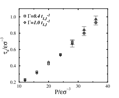
FIG. 2.: Yield stress vs. pressure for two values of the parameter $\Gamma$ that controls the rate of heat exchange with the thermostat (Equation 5). We observed no influence of the thermostat on the yield stress. For this data, the coverage is 1/2, $\theta=90^{\circ}$, $\sigma_{\rm wf}=1.0\sigma$, $\epsilon_{\rm wf}=1.0\epsilon$, $r_{\rm c}=2^{1/6}\sigma$, $d_{\rm nn}=1.2\sigma$, $T=0.7\epsilon/k_{B}$ and $n$=6. The search algorithm was used, and the simulation cell was 28.8$\sigma$ by 24.9$\sigma$. Error bars are indicated when they are bigger than the symbol size.

B Effect of system size

The phenomenological expressions for friction described in the introduction assume that the static friction is given by a yield stress times the area of contact. The regions of direct molecular contact between macroscopic solids typically have diameters of order microns.[17, 18, 19, 22] It is important to establish that yield stresses calculated at the much smaller scales of our simulations are representative of larger contacts. It is also interesting to consider how friction forces would change if the contact dimensions were reduced to nanometer scales.

Figure 3 compares results from the ramp and search algorithms and shows how both scale with contact size. Values of the yield stress $\tau_{\rm s}$ at $P=12$ and $28\epsilon\sigma^{-3}$ are plotted as a function of the inverse width of the simulation cell. The latter is expressed as $A^{-1/2}$ where $A$ is the area in the x-y plane. Given $\sigma\sim 0.5$nm, the largest contact widths (smallest values of $A^{-1/2}$) correspond to 50nm and the smallest widths to about 10nm.

We first consider how contact area affects the variations in the stress needed to initiate sliding from different initial configurations. Points indicated by stars and squares indicate the maximum and mean forces needed to initiate sliding for $P=28\epsilon\sigma^{-3}$ with the ramp algorithm. Note that the difference between the extreme and average yield stresses decreases rapidly with system size and is about 10% for the largest systems. This indicates that the distribution of yield stresses is well-behaved and can be thought of as arising from an incoherent sum of contributions from different regions of the contact. The same trend is seen for the maximum and mean values from the search algorithm, but the fluctuations are slightly smaller.

In both algorithms the smallest system sizes tend to produce larger mean stresses. However, as assumed in phenomenological theories of friction,[11, 15, 17] the mean values of the yield stress for all pressures and algorithms go to well defined limits as the contact size diverges. As shown in Fig. 3, finite size effects are larger for higher pressures. This may be because the energy barrier for monomers to move between metastable states increases with pressure, making them more likely to get stuck in high energy states. Finite-size effects also grow rapidly as the coverage decreases, since there are then fewer monomers at the same wall area.

Note that yield stresses from the ramp algorithm tend to be consistently higher than those from the search algorithm. At $P=28\epsilon\sigma^{-3}$ the difference appears to reflect larger finite-size effects for the ramp algorithm. However the difference between the two algorithms is nearly independent of system size for $P=12\epsilon\sigma^{-3}$. The reason for this discrepancy is that it takes time for the wall to accelerate once the static friction is exceeded. One can only be sure that the wall has started sliding when it has moved by a few $\sigma$. With the ramp algorithm the force has increased to a higher value by this point. Attempts to extrapolate back to the onset of motion only partially corrected for this offset. Decreasing the ramp rate reduces the error, but also lengthens the simulation time proportionately. The search algorithm reduces the effective ramp rate to zero and efficiently converges on the yield stress.

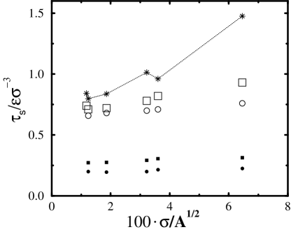
FIG. 3.: Mean yield stress as a function of the inverse square root of the area $A$ of the periodic simulation cell for the ramp (squares) and search (circles) algorithms at $P=12\epsilon\sigma^{-3}$ (closed symbols) and $P=28\epsilon\sigma^{-3}$ (open symbols). The maximum stress needed to initiate sliding from any initial condition at $P=28\epsilon\sigma^{-3}$ is indicated by asterisks for the ramp algorithm. Simulations were done with rigid walls at $1/2$ coverage, $\theta=90^{\circ}$, $\sigma_{\rm wf}=\sigma$, $\epsilon_{\rm wf}=\epsilon$, $r_{\rm c}=2^{1/6}\sigma$, $d_{\rm nn}=1.2\sigma$, $T=0.7\epsilon/k_{B}$ and $n=6$. Statistical errors are indicated by the symbol size.

For the above reasons the search algorithm is used for most of the following plots. Except where noted, the second to smallest system size of Figure 3 is used. The surface of each wall then has 576 atoms and the simulation cell is 28.8$\sigma$ by 24.94$\sigma$ for the usual case of $d_{\rm nn}=1.2\sigma$. Larger system sizes are used mainly at low coverage in order to ensure that the deviation of the yield stress from the thermodynamic limit is comparable to statistical uncertainties. Larger systems also allow a greater number of rotation angles, $\theta$, to be studied.

C Effect of temperature and pressure

Figure 4 shows the yield stress vs. pressure for a coverage of 1/2 over a broad temperature range from $k_{B}T/\epsilon=0.3$ to $1.3$. For reference, the triple point and critical temperature of Lennard-Jones monomers with $r_{\rm c}\rightarrow\infty$ are about 0.7 and 1.3 $\epsilon/k_{B}$, respectively,[58, 62] and the zero pressure glass transition temperature for short Lennard-Jones chains is between 0.4 and 0.5$\epsilon/k_{B}$.[63, 64, 65]

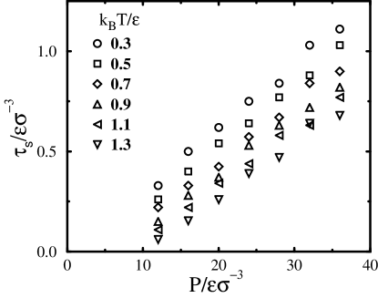
FIG. 4.: Variation of yield stress with pressure at the indicated temperatures. In each case, $\tau_{\rm s}$ rises linearly with $P$. The size of typical statistical errors is indicated by the symbol size. Errors are slightly larger at the highest pressures. Simulations were done with the search algorithm for rigid walls, $1/2$ coverage, $\theta=90^{\circ}$, $\sigma_{\rm wf}=\sigma$, $\epsilon_{\rm wf}=\epsilon$, $r_{\rm c}=2^{1/6}\sigma$, $d_{\rm nn}=1.2\sigma$, and $n$=6.

Note that $\tau_{\rm s}$ increases linearly with pressure at each $T$, as assumed in Equation 1. For representative values of $\epsilon$=30meV and $\sigma=0.5$nm, the unit of pressure $\epsilon\sigma^{-3}\sim$40MPa. Thus the highest pressures in Figure 4 correspond to about 1.5GPa. In those cases that we checked, linearity extended up to much larger pressures (at least 100$\epsilon\sigma^{-3}$). However, these pressures were not routinely studied because a smaller time step is needed to integrate the equations of motion at larger pressures.

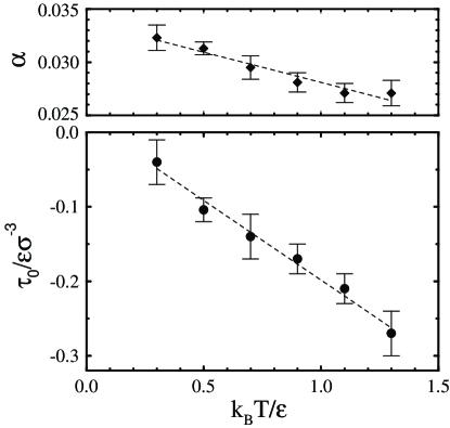
FIG. 5.: Values of $\alpha$ and $\tau_{0}$ as a function of temperature from fits of Equation 1 to the data of Figure 4. Dashed lines show the linear fits to the temperature dependence given in Equation 6.

The plots of yield stress vs. pressure at different temperatures in Figure 4 are nearly parallel, but their intercepts shift rapidly with temperature. Results from fits to Equation 1 are shown in Figure 5. The slope $\alpha$ drops by only 16% with increasing $T$, while the intercept $\tau_{0}$ is roughly proportional to $T$. Linear fits as a function of temperature give:

$$\begin{array}[]{lll}\alpha&=&(-0.0057\pm 0.0007)\frac{k_{B}T}{\epsilon}+(0.0338\pm 0.0006)\\ \frac{\tau_{0}}{(\epsilon\sigma^{-3})}&=&(-0.214\pm 0.013)\frac{k_{B}T}{\epsilon}+(0.015\pm 0.011).\end{array}$$ (6)

An explanation for the nearly constant value of $\alpha$ is presented in Section III F. In the remainder of this subsection we focus on the variation of $\tau_{0}$.

At each $T$, the linear fit for yield stress vs. pressure crosses through zero at a threshold pressure $P_{\rm t}=-\tau_{0}/\alpha$. Above this pressure we find a well defined yield stress in the thermodynamic limit. Below $P_{\rm t}$, the adsorbed layer acts like a lubricating liquid, with a shear stress that vanishes as the shear rate decreases.[48] In this regime, the bounding walls are far enough apart that molecules diffuse freely and do not lock the two walls in a local energy minimum. From the fit parameters in Fig. 6 we see that $P_{\rm t}$ rises roughly linearly with $T$. This is because the simulations used $r_{\rm c}=2^{1/6}\sigma$, which corresponds to the hard sphere limit. In this regime pressures are balanced only by entropic forces and thus must scale linearly with temperature. Attractive interactions are considered in Sec. III F

Most of the following simulations were done at $T=0.7\epsilon/k_{B}$. Given the results just described, we expect that the same trends would be observed at other temperatures.

D Effect of wall stiffness

As described in Section II A, wall atoms were connected to lattice sites by springs with stiffness $k_{\rm s}$, or fixed rigidly to these sites ($k_{\rm s}\rightarrow\infty$). Decreasing $k_{\rm s}$ has two competing effects on the static friction. One is to make it easier for the two surfaces to deform into a structure with a common period. This tends to increase the yield stress. However, studies with bare walls found that unrealistically small values of $k_{\rm s}$ were needed to produce a finite static friction.[34] Decreasing $k_{\rm s}$ also decreases the yield stress by allowing wall atoms to be pushed out of the way. In our simulations the second effect always dominates, and $\tau_{\rm s}$ decreases as $k_{\rm s}$ decreases. This is consistent with a recent analytic theory for static friction.[38]

Fig. 6 shows results for systems $C$ and $D$ of Fig. 1 at $k_{B}T=0.7\epsilon$. In each case, the yield stress rises linearly with pressure and decreases monotonically with $k_{\rm s}$. The value of $\alpha$ drops by up to 50% as $k_{\rm s}$ decreases from infinity to $210\epsilon\sigma^{-3}$. Note that for $k_{\rm s}=210\epsilon\sigma^{-3}$ the rms displacement about lattice sites is near the usual Lindemann criterion for melting, [54] so much weaker values would be unphysical. To minimize computer time and the number of free parameters, we used rigid walls $k_{\rm s}\rightarrow\infty$ in the following sections.

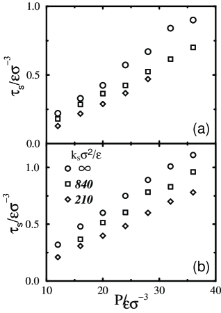
FIG. 6.: Yield stress vs. pressure for the indicated values of the stiffness $k_{\rm s}$ of the springs coupling wall atoms to lattice sites. The top panel shows results for $\theta=90^{\circ}$ (Fig. 1C) and the bottom panel shows results for $\theta=0^{\circ}$ but $d/d^{\prime}=12/13$ (Fig. 1D). In each case, decreasing the stiffness decreases the yield stress. These results are from the search algorithm with $1/2$ coverage, $\sigma_{\rm wf}=\sigma$, $\epsilon_{\rm wf}=\epsilon$, $r_{\rm c}=2^{1/6}\sigma$, $d_{\rm nn}=1.2\sigma$, and $n$=6.

E Effect of wall orientation, coverage and chain length

Calculated values of the static friction for bare surfaces vary dramatically with wall geometry.[7, 32, 66] The yield stress equals that of a bulk crystal for identical aligned surfaces ($\theta=0^{\circ}$) and is identically zero for incommensurate orientations. Most experiments do not control the wall orientation, and yet measured friction coefficients between nominally dry surfaces vary by roughly 10% within the same laboratory and by 20% between laboratories.[22, 67] Another factor that is not controlled in most experiments is the density and chemistry of adsorbed molecules, although humidity is controlled in some cases. If adsorbed molecules are crucial in determining the static friction, the friction they produce must be relatively insensitive to the wall orientation, sliding direction, coverage and chain length.

Figure 7 shows the yield stress as a function of pressure for the different walls shown in Figure 1. At low coverages (Fig. 7(a)), the friction is nearly identical for all incommensurate walls. The friction for commensurate walls is roughly four times higher, but much less than the value for bare walls. At a coverage of 1/2 (Fig. 7(b)), the difference in the yield stresses for different incommensurate walls increases to roughly 20%. A similar variation with the direction of sliding ($\phi=0$ or 90^∘) is seen. Most of this variation is due to changes in $\tau_{0}$ and all the curves are nearly parallel. Fit values of $\alpha$, which dominates the high pressure friction, only change by about 5%.

The greater variability at coverage of 1/2 arises because this case corresponds to a dense monolayer between the surfaces. Molecules can not pick and choose which portions of the surface to cover. As a result the friction is higher for geometries B and D, where there are larger regions where the walls look commensurate and molecules can easily lock in registry with both surfaces. The friction is smallest for geometry C, where there is almost no region where the two walls are in registry.

Figure 8 shows the yield stress vs. pressure at different coverages for the extreme case of geometry C ($\theta=90^{\circ}$). Note that the yield stress exhibits the usual linear pressure dependence at all coverages, and that most of the variation with coverage is in the intercept $\tau_{0}$. The value of $\alpha$ stays within 15% of the mean value, 0.030. At each pressure, the friction decreases as the coverage rises from 1/8 to 1/2. During this increase in coverage, more and more of the sites with poor registry must be occupied. The friction goes down to a minimum value at a complete monolayer which corresponds to about 1/2 coverage. If the difference between the sizes of the monomers and wall atoms was bigger, locking would be frustrated even in the areas with good registry. This might lead to even smaller variations with coverage than those shown here.

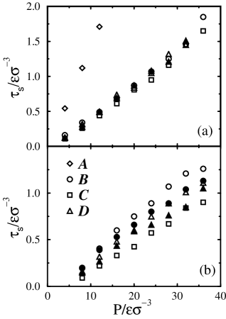
FIG. 7.: Shearing direction and orientation dependence for (a) 1/8 coverage and (b) 1/2 coverage. The symbol shape indicates which of the geometries in Fig. 1 were used (see legend). Open and closed symbols are for lateral force applied along the $x$ ($\phi=0^{\circ}$) and $y$ ($\phi=90^{\circ}$) directions, respectively. The ramp algorithm was used in (a) and the search algorithm was used in (b). The potential parameters were $\sigma_{\rm wf}=\sigma$, $\epsilon_{\rm wf}=\epsilon$, $r_{\rm c}=2^{1/6}\sigma$, $d_{\rm nn}=1.2\sigma$, and $n$=6.

As coverage rises from 1/2 to 1 (about two monolayers), the friction rises once more. The reason is that two layers of molecules have more internal degrees of freedom and can lock more easily into simultaneous registry with both walls. For this range of coverages yield continues to localize at the surfaces of the walls. Previous work on thicker films shows that yield can move into the film as thickness increases.[68, 69] In this limit $\tau_{\rm s}$ approaches the bulk yield stress of the material making up the adsorbed layer, and eventually becomes independent of the coverage. Note that the bulk yield stress of polymeric materials is also found to follow the linear pressure dependence of Equation 1. [60]

Figure 9 illustrates the interplay between the chain length and coverage dependence. At small coverages (Fig. 9 (a)), there is little dependence on chain length or wall orientation. For a complete monolayer (Fig. 9 (b)), chains with $n=3$ and $6$ show nearly the same behavior, while spherical molecules ($n=1$) show a dramatically reduced friction and $\alpha$. This suggests that the spheres are more constrained by their neighbors from locking into registry with the walls. This may reflect the fact that although all films contain the same number of monomers at a coverage of 1/2, the spheres are closer to their true equilibrium monolayer density than the chains. The reason is that the strong bonds within chain molecules lower the equilibrium spacing and thus increase the equilibrium density at a given pressure. The presence of two different types of bonds in chain molecules may also improve their ability to rearrange to lock into both surfaces. Another possibility is that chains produce a greater friction because of the strong intramolecular bonds. If one monomer in the chain is locked to the bottom wall and another is in registry with the top wall, the intramolecular bonds will lock the two walls together. This process has no analog for monomers and is particularly important as the coverage increases beyond a monolayer.

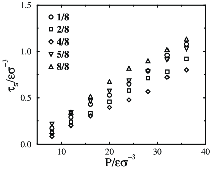
FIG. 8.: Yield stress vs. pressure for the indicated coverages with system C ($\theta=90^{\circ}$) where the largest variation was observed. Note that a coverage of 1/2 on each separated surface produces about a monolayer when the surfaces are placed in contact. Results are from the search algorithm with $\sigma_{\rm wf}=\sigma$, $\epsilon_{\rm wf}=\epsilon$, $r_{\rm c}=2^{1/6}\sigma$, $d_{\rm nn}=1.2\sigma$, and $n$=6.

Figure 10 shows the static friction as a function of $\theta$ at a single pressure, $P=24\epsilon\sigma^{-3}$. This large pressure was chosen to maximize the contribution of $\alpha$ to the yield stress. Only $\theta$ between 0 and 30^∘ are shown because other angles are related by symmetry.

The commensurate case $\theta=0^{\circ}$ shows a much larger friction than any of the incommensurate systems. Even a $2^{\circ}$ rotation reduces the friction to a value that is comparable to those at other values of $\theta$. The same sharp transition was seen for coverages from 1/8 to 1. The data shown is for coverage of 1/2 where the variation of the yield stress at incommensurate $\theta$ has already been shown to be largest. Even in this case the variation is less than $\pm 20$%, which is comparable to experimental variations. The smaller variations of yield stress with $\theta$ at a coverage of 1/8 are comparable to our statistical errorbars.

The sliding direction $\phi$ also has relatively little influence on the yield stress between incommensurate surfaces. Two orthogonal directions $\phi=0^{\circ}$ and 90^∘ are shown in Fig. 10. The difference between them is most pronounced at small $\theta$, where $\phi=0^{\circ}$ corresponds to pulling nearly parallel to the nearest-neighbor direction in each wall, and $\phi=90^{\circ}$ to pulling along the perpendicular direction.

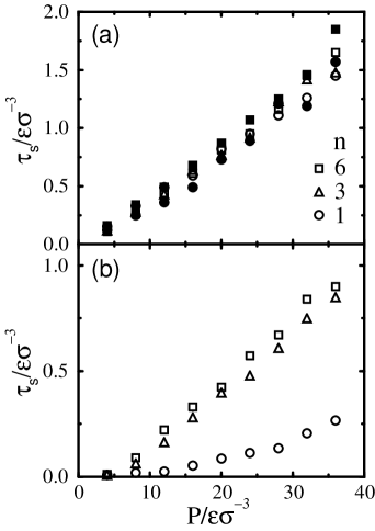
FIG. 9.: Yield stress vs. pressure for the indicated values of chain length $n$ at coverage of (a) $1/8$ and (b) $1/2$. Open (closed) symbols are for system C (B). The potential parameters were $\sigma_{\rm wf}=\sigma$, $\epsilon_{\rm wf}=\epsilon$, $r_{\rm c}=2^{1/6}\sigma$, and $d_{\rm nn}=1.2\sigma$. Errorbars are comparable to the system size and the ramp (search) algorithm was used for the top (bottom) panel. Except for spherical molecules at $1/2$ coverage, the friction is insensitive to chain length.

Figure 11 shows the variation with $\phi$ in more detail for coverage of 1/2 and $\theta=10.4^{\circ}$, where the variation in Fig. 10 is large. The data are symmetric about $\theta/2$ which is the direction of a 2-fold axis. This direction gives the maximum friction, and the yield stress drops to a plateau value on either side. The variation is within our statistical errors at low pressures and is less than $\pm 20$% at the largest pressures studied. As in Figures 7(b) and 10, sliding along the x axis leads to higher friction than sliding along y (equivalent to $\phi=0$ and $30^{\circ}$, respectively).

Note that when the yield stress is exceeded the top wall does not always move exactly in the direction of the applied force. This effect is most pronounced for the commensurate case, but is also seen at small $\theta$.

F Effect of Interaction Potentials

Experimental results for different sliding surfaces and different surface layers show much larger variations than the fluctuations for a given material system. Such changes in material would correspond to changes in the parameters in our interaction potentials such as the strength of the interaction between the wall and fluid $\epsilon_{\rm wf}$, the characteristic length of this interaction $\sigma_{\rm wf}$, the range of the interaction $r_{\rm c}$, and the nearest-neighbor spacing $d_{\rm nn}$ in the walls. Other structural properties and the elastic moduli and hardness of the solids may also be important, but are not easily included within our model.

FIG. 10.: Yield stress as a function of orientation angle $\theta$ at $P=24\epsilon\sigma^{-3}$. The commensurate case corresponds to $\theta=0$ and the smallest non-zero angle shown here is $2.02^{\circ}$. These results are from the search algorithm with $1/2$ coverage, $\sigma_{\rm wf}=\sigma$, $\epsilon_{\rm wf}=\epsilon$, $r_{\rm c}=2^{1/6}\sigma$, $d_{\rm nn}=1.2\sigma$, and $n$=6. The simulation cell was $57.6\sigma$ by $49.9\sigma$.

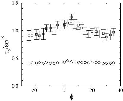
FIG. 11.: The yield stress vs. the angle $\phi$ between the applied stress and the $x$ axis for $P=12\epsilon\sigma^{-3}$ (circles) and 32$\epsilon\sigma^{-3}$ (squares). These results are from the search algorithm with $1/2$ coverage, $\sigma_{\rm wf}=\sigma$, $\epsilon_{\rm wf}=\epsilon$, $r_{\rm c}=2^{1/6}\sigma$, $d_{\rm nn}=1.2\sigma$ and $n=6$. The simulation cell was $57.6\sigma$ by $49.88\sigma$. Errorbars are only shown when they are larger than the symbol size.

The results shown so far were all for purely repulsive potentials, $r_{\rm c}=2^{1/6}\sigma$. Increasing the cutoff to $r_{\rm c}=2.2\sigma$ includes most of the attractive tail in the Lennard-Jones potential. This attractive tail leads to an adhesive force pulling the walls together in addition to the external pressure $P$. As shown in Fig. 12(a) and (c), the yield stress for $r_{\rm c}=2.2\sigma$ is parallel to results for $r_{\rm c}=2^{1/6}\sigma$ and could be obtained by shifting the zero of pressure to reflect the adhesive stress. The required shift increases with increasing coverage because the density of adsorbed molecules that contribute to the adhesive interaction increases.

When the above results are fit to Eq. 1, the value of $\alpha$ is independent of $r_{\rm c}$, and the value of $\tau_{0}$ increases with the amount of adhesion. For purely repulsive interactions $\tau_{0}$ is negative because a finite pressure is needed to lock the adsorbed layers in a glassy state (Sec. III C). When $r_{\rm c}$ is increased to 2.2$\sigma$, a glass forms at zero pressure, and the value of $\tau_{0}$ is positive. Many authors refer to $\tau_{0}$ as the adhesive contribution to friction, and it is obvious that $\tau_{0}/\alpha$ represents the effective adhesive pressure that must be added to the external pressure to get strict proportionality between the friction and total load.

These simulations did not include the direct interactions between atoms from different walls. As noted in Section II A, the wall spacing is large enough that the direct interaction vanishes for $r_{\rm c}=2^{1/6}\sigma$. Even for $r_{\rm c}=2.2\sigma$, wall interactions have little effect. For example the extra adhesive pressure due to wall/monomer interactions is $\tau_{0}/\alpha\sim 5\epsilon\sigma^{-3}$ for 1/2 coverage (Fig. 12(a)). Direct calculation of the extra adhesive pressure due to interactions between atoms on different walls yields a value that rises from 0.4 to 1.3$\epsilon\sigma^{-3}$ over the observed range of wall separations. Correcting the external pressure to account for this interaction would change $\alpha$ by less than 3%.

Panels (b) and (c) of Fig. 12 show that doubling the strength of the potential between the surfaces and monomers has almost no effect on the yield stress. The main factor that changes $\alpha$ is the ratio between the characteristic separation between wall and fluid atoms, $\sigma_{\rm wf}$, and the nearest-neighbor spacing between wall atoms, $d_{\rm nn}$. The value of $\alpha$ rises monotonically as $\sigma_{\rm wf}/d_{\rm nn}$ decreases. For the cases shown, $\alpha$ changes by an order of magnitude. Smaller values of $\alpha$ are obtained by increasing $\sigma_{\rm wf}/d_{\rm nn}$ further, but it is difficult to increase $\alpha$ for this geometry. The reason is that the adsorbed molecules begin to penetrate into the wall when $\sigma_{\rm wf}/d_{\rm nn}$ is too small. Other crystallographic orientations of the surface, such as (100), may produce larger values of $\alpha$. Flat but disordered surfaces produce values of $\alpha$ as high as 0.3.[38, 47]

The strong effect of $\sigma_{\rm wf}/d_{\rm nn}$ and weak effect of $\epsilon_{\rm wf}/\epsilon$ suggest a geometric origin of $\alpha$ that is analogous to early geometric theories for Amontons’ laws [10] and to Israelachvili’s cobblestone model.[15, 23] At pressures where the adsorbed layer acts like a glass, the repulsive part of the Lennard-Jones interaction dominates. The repulsive force between monomers and wall atoms at a separation $r$ is given by $F_{\rm rep}=48(\epsilon_{\rm wf}/\sigma_{\rm wf})(\sigma_{\rm wf}/r)^{13}$. The mean value of $F_{\rm rep}$ must scale with the pressure. Hence, increasing $P$ by a factor of 2 only decreases the typical separation between monomers and wall atoms by a factor of $2^{1/13}$ or 5%. Increasing $\epsilon_{\rm wf}$ by a factor of two leads to the same small decrease in separation. In contrast, the separation changes by a factor of $2^{12/13}\approx 1.9$ with a factor of 2 change in $\sigma_{\rm wf}$. Thus monomers and wall atoms can be thought of as hard spheres whose diameter $D$ is nearly independent of pressure and $\epsilon_{\rm wf}$ but directly proportional to $\sigma_{\rm wf}$.

Figure 13 illustrates the effect of changing the ratio between the hard sphere diameter and the nearest-neighbor spacing $d_{\rm nn}$. The hard-sphere repulsion leads to a surface of closest approach between a monomer and the wall. In order for the monomer to slide relative to the wall it must be lifted up the ramp formed by this surface. The lateral force required to move monomers up the ramp is just the normal load times the slope of the surface. Thus $\alpha$ will be proportional to some average of the slope over all monomers. As $D/d_{\rm nn}$ decreases, monomers penetrate more deeply between the surfaces and both the slope and $\alpha$ increase. This is precisely the trend seen in Fig. 12. Thus the hard-sphere model explains the linear dependence of $\tau$ on pressure as well as the insensitivity to $\epsilon_{\rm wf}$ and the variation with $\sigma_{\rm wf}$ and $d_{\rm nn}$.

FIG. 12.: Yield stress vs. pressure for various choices of the potential parameters in system C with $n=6$. The coverage is $1/2$ in (a) and (b) and $1/8$ in (c). Unless noted the default values of $\sigma_{\rm wf}=\sigma$, $\epsilon_{\rm wf}=\epsilon$, $d_{\rm nn}=1.2\sigma$, and $r_{\rm c}=2^{1/6}\sigma$ are used. Each of these parameters was changed in turn and the corresponding results are labeled by the changed value. The search algorithm was used for the data in (a) and (b), and the ramp algorithm was used in (c).

FIG. 13.: Sketch of surface of closest approach for $D/d_{\rm nn}=0.7$ (solid line) and 1.3 (dashed line). The lateral force required to lift monomers up the ramps that these surfaces represent is given by the slope times the normal force.

IV Summary and Conclusions

The results presented in this paper explore the effect of a specific type of third-body, small adsorbed molecules, on the friction between the bounding solids. The effect of temperature, coverage, crystalline alignment, lattice constant, system size, molecular size and interaction potential parameters were all examined.

The first important result is that static friction is observed for all systems – even when the static friction between bare walls is identically zero. The shear stress needed to initiate sliding approaches a constant value in the thermodynamic limit (Fig. 3) and follows the linear pressure dependence (Equation 1) seen in many experimental systems. Moreover, the shear stress is insensitive to parameters that are not controlled in most experiments, including crystalline alignment, coverage and sliding direction. Even under conditions where the variations with these parameters are largest, the changes are comparable to typical experimental variations between different samples and laboratories.[22, 67] This is an important test of any molecular scale model for friction.

The value of $\tau_{0}$ in Equation 1 is increased by attractive interactions between the monomers and walls or between the two walls. The adhesive interaction was increased both by increasing coverage (Fig. 8) and by increasing $r_{c}$ to increase the contribution from the attractive tail in the Lennard-Jones potential (Fig. 12). Increasing the temperature (Fig. 5) increases the entropic repulsion and lowers $\tau_{0}$.

For each system there is a pressure $P_{t}=-\tau_{0}/\alpha$ below which the adsorbed layer acts like a liquid lubricant (Sec. III C). When the attractive tail of the Lennard-Jones potential is included (large $r_{c}$), the value of $P_{t}$ for submonolayer films is negative up to quite high temperatures. This suggests that thicker films are needed to achieve lubricated behavior in typical experimental systems. However, it would be interesting to explore whether the static friction between flat surfaces can be eliminated by the proper choice of molecule and the use of elevated temperatures.

All of the observed trends in $\alpha$ can be understood in terms of a simple geometrical model where monomers act like hard spheres. Within this model, $\alpha$ only depends on the hard sphere diameter and the wall geometry. Parameters such as pressure, temperature, wall/monomer coupling energy, and $r_{c}$ have almost no effect on the hard sphere diameter and thus $\alpha$. In contrast, changes in $\sigma_{\rm wf}$ or $d_{\rm nn}$ produce direct changes in the geometry and change $\alpha$ dramatically (Fig. 12). Smaller shifts in $\alpha$ are produced by changes in coverage that alter the ability of the hard spheres to pack into a configuration that locks into both walls (Fig. 8).

Simple model potentials were used for the adsorbed molecules and surfaces in this study, in order to allow a wide range of parameters to be investigated. More realistic models will have more complex interactions and multiple atomic species. This will complicate the geometry, but one expects that the basic idea of an effective surface of closest approach defined by hard-sphere repulsions will still be valid at the pressures of interest. This naturally produces static friction and a shear stress that obeys Equation 1. Indeed the same picture can be applied to larger particles between bearing surfaces such as dust, sand or wear debris.

While our geometric argument for $\alpha$ bears some similarity to earlier models based on interlocking of macroscopic[10] or atomic[15, 23] asperities, there is an important difference. These previous models envisioned asperities that were rigidly attached to their respective surfaces and would translate with them. The mobile atoms considered here and in previous work,[34, 38, 47, 48] rearrange to create interlocking configurations for any relative position of the surfaces. Not only does this explain why static friction can occur between surfaces with uncorrelated asperities, it also makes it possible to connect static and kinetic friction.

As pointed out by Leslie[10] in 1804, interlocking of rigid asperities can explain static friction, but predicts vanishing kinetic friction. The reason is that the energy needed to move up ramps is recovered as the asperities move back down and the total work required to slide the surfaces vanishes. The situation is very different when the interlocking occurs dynamically through motion of adsorbed molecules. As shown in recent work,[38, 48] at any given instant almost all of the mobile molecules are trapped in local free energy minima. Since lateral motion of the walls increases their energy within this minimum they contribute to the friction. The kinetic and static friction are closely related because the distribution of molecules in free energy minima is nearly the same. The difference is that when the walls are moving at fixed velocity the minimum holding each molecule eventually becomes unstable. It then pops forward rapidly to the nearest metastable state. Much of its energy is dissipated in this pop because molecules pop forward at different locations at different times in an incoherent manner and the potential they move to varies in a random way. It is not possible for them to move up and down over a rigid potential energy surface as in the models of fixed asperities considered by Leslie and earlier researchers.[10]

REFERENCES

- [1] R. W. Carpick and M. Salmeron, Chem. Rev. 97, 1163 (1997).
- [2] J. Krim, Scientific American 275(4), 74 (1996).
- [3] S. Granick, Science 253, 1374 (1992).
- [4] M. L. Gee, P. M. McGuiggan, J. N. Israelachvili, and A. M. Homola, J. Chem. Phys. 93, 1895 (1990).
- [5] C. F. McFadden and A. J. Gellman, Surf. Sci. 409, 171 (1998).
- [6] Handbook of Micro/Nanotribology, edited by B. Bhushan (CRC, Boca Raton, 1999).
- [7] M. O. Robbins and M. H. Müser, in Modern Tribology Handbook: Vol. 1 Principles of Tribology, edited by B. Bhushan (CRC Press, Boca Raton, 2000 (cond-mat/0001056)), pp. 717–765.
- [8] J. A. Harrison, S. J. Stuart, and D. W. Brenner, in Handbook of Micro/Nanotribology, edited by B. Bhushan (CRC Press, Boca Raton, 1999), pp. 525–594.
- [9] M. O. Robbins and E. D. Smith, Langmuir 12, 4543 (1996).
- [10] D. Dowson, History of Tribology (Longman, New York, 1979), pp. 153–67.
- [11] B. J. Briscoe and D. Tabor, J. Adhesion 9, 145 (1978).
- [12] B. J. Briscoe, Phil. Mag. A 43, 511 (1981).
- [13] B. J. Briscoe and A. C. Smith, Trans. ASLE 25, 349 (1982).
- [14] I. L. Singer in Fundamentals of Friction: Macroscopic and Microscopic Processes, edited by I. L. Singer and H. M. Pollock (Elsevier, Amsterdam, 1992), pp. 237–261.
- [15] A. Berman, C. Drummond, and J. N. Israelachvili, Tribology Letters 4, 95 (1998).
- [16] A. L. Demirel and S. Granick, J. Chem. Phys. 109, 6889 (1998).
- [17] F. P. Bowden and D. Tabor, The Friction and Lubrication of Solids (Clarendon Press, Oxford, 1986).
- [18] J. H. Dieterich and B. D. Kilgore, Tectonophysics 256, 219 (1996).
- [19] P. Berthoud and T. Baumberger, Proc. R. Soc. Lond A 454, 1615 (1998).
- [20] J. A. Greenwood and J. B. P. Williamson, Proc. Roy. Soc. A 295, 300 (1966).
- [21] A. Volmer and T. Natterman, Z. Phys. B 104, 363 (1997).
- [22] E. Rabinowicz, Friction and Wear of Materials (Wiley, New York, 1965).
- [23] J. N. Israelachvili, S. Giasson, T. Kuhl, C. Drummond, A. Berman, G. Luengo, J.-M. Pan, M. Heuberger, W. Ducker and M. Alcantar, in Thinning films and tribological interfaces (Elsevier, New York, 2000), Vol. Tribology Series 38, pp. 3–12.
- [24] Y. I. Frenkel and T. Kontorova, Zh. Eksp. Teor. Fiz. 8, 1340 (1938).
- [25] S. Aubry, in Solitons and Condensed Matter Physics, edited by A. R. Bishop and T. Schneider (Springer-Verlag, Berlin, 1979), pp. 264–290.
- [26] P. Bak, Rep. Progr. Phys. 45, 587 (1982).
- [27] G. M. McClelland, in Adhesion and Friction, edited by M. Grunze and H. J. Kreuzer (Springer Verlag, Berlin, 1989), Vol. 17, pp. 1–16.
- [28] M. Hirano and K. Shinjo, Phys. Rev. B 41, 11837 (1990).
- [29] K. Shinjo and M. Hirano, Surface Science 283, 473 (1993).
- [30] B. N. J. Persson, Phys. Rev. B 48, 18140 (1993a).
- [31] M. Cieplak, E. D. Smith, and M. O. Robbins, Science 265, 1209 (1994).
- [32] M. R. Srensen, K. W. Jacobsen, and P. Stoltze, Phys Rev. B 53, 2101 (1996).
- [33] E. D. Smith, M. Cieplak, and M. O. Robbins, Phys. Rev. B. 54, 8252 (1996).
- [34] M. H. Müser and M. O. Robbins, Phys. Rev. B 61, 2335 (2000).
- [35] J. A. Harrison, C. T. White, R. J. Colton, and D. W. Brenner, Phys. Rev. B 46, 9700 (1992b).
- [36] J. A. Harrison, R. J. Colton, C. T. White, and D. W. Brenner, Wear 168, 127 (1993).
- [37] Note that cold welding leading to static friction is observed between some clean metal surfaces. It may be that this is driven by plastic deformation or that long experimental time scales allow diffusion to reconstruct the interface into locally commensurate grain boundaries with different orientations.
- [38] M. H. Müser, L. Wenning, and M. O. Robbins, Phys. Rev. Lett. 86, 1295 (2001 and cond-mat/0004494).
- [39] C. Caroli and P. Nozieres, in Physics of Sliding Friction, edited by B. N. J. Persson and E. Tosatti (Kluwer, Dordrecht, 1996), pp. 27–49.
- [40] B. N. J. Persson and E. Tosatti, in Physics of Sliding Friction, edited by B. N. J. Persson and E. Tosatti (Kluwer, Dordrecht, 1996), pp. 179–189.
- [41] J. Krim, E. T. Watts, and J. Digel, J. Vac. Sci. Technol. A 8, 3417 (1990).
- [42] J. Krim, D. H. Solina, and R. Chiarello, Phys. Rev. Lett. 66, 181 (1991).
- [43] M. Hirano, K. Shinjo, R. Kaneko, and Y. Murata, Phys. Rev. Lett. 78, 1448 (1997).
- [44] M. Hirano, K. Shinjo, R. Kaneko, and Y. Murata, Phys. Rev. Lett. 67, 2642 (1991).
- [45] J. M. Martin, C. Donnet, T. L. Mogne, and T. Epicier, Phys. Rev. B 48, 10583 (1993).
- [46] J. S. Ko and A. J. Gellman, Langmuir 16, 8343 (2000).
- [47] G. He, M. H. Müser, and M. O. Robbins, Science 284, 1650 (1999).
- [48] G. He and M. O. Robbins, Trib. Lett. 10, 7-14 (2001), cond-mat/0008196.
- [49] M. Godet, Wear 100, 437 (1984).
- [50] Y. Berthier, M. Brendle, and M. Godet, STLE Tribology Trans. 32, 490 (1989).
- [51] Note that even if the layer responded elastically one would expect pinning to occur since elastic two-dimensional systems are always pinned by disorder. (See for example G. Grüner, Rev. Mod. Phys. 60, 1129 (1988).)
- [52] K. Kremer and G. S. Grest, J. Chem. Phys. 92, 5057 (1990).
- [53] P. A. Thompson and M. O. Robbins, Phys. Rev. A 41, 6830 (1990).
- [54] The Lindemann criterion for melting corresponds to an root-mean-square displacement about lattice sites of about 15% of the nearest neighbor spacing. See for example J. P. Hansen and I. R. McDonald, Theory of Simple Liquids (Academic, New York, 1986), 2nd ed. or M. J. Stevens and M. O. Robbins, J. Chem. Phys. 98, 2319 (1993).
- [55] M. Weiss and F.-J. Elmer, Phys. Rev. B 53, 7539 (1996).
- [56] G. S. Grest and K. Kremer, Phys. Rev. A 33, 3628 (1986).
- [57] A. Liebsch, S. Gonçalves, and M. Kiwi, Phys. Rev. B 60, 5034 (1999).
- [58] M. P. Allen and D. J. Tildesley, Computer Simulation of Liquids (Clarendon Press, Oxford, 1987).
- [59] Note that if long-range elasticity were included in the walls one might have a limiting barrier at large wall areas due to activation of independent regions.
- [60] See for example I. M. Ward, Mechanical Properties of Solid Polymers (Wiley, New York, 1983).
- [61] The stress is increased to this value over 10.
- [62] B. Smit, J. Chem. Phys. 96, 8639 (1992).
- [63] A. R. C. Baljon and M. O. Robbins, in Micro/Nanotribology and Its Applications, edited by B. Bhushan (Kluwer, Dordrecht, 1997), pp. 533–553.
- [64] M. O. Robbins and A. R. C. Baljon, in Microstructure and Microtribology of Polymer Surfaces, edited by V. V. Tsukruk and K. J. Wahl (American Chemical Society, Washington DC, 2000), pp. 91–117.
- [65] C. Bennemann, W. Paul, K. Binder, and B. Dünweg, Phys. Rev. E 57, 843 (1998).
- [66] M. Hirano and K. Shinjo, Wear 168, 121 (1993).
- [67] H. Czichos, S. Becker, and J. Lexow, Wear 135, 171 (1989).
- [68] P. A. Thompson, M. O. Robbins, and G. S. Grest, Israel J. of Chem. 35, 93 (1995).
- [69] E. Manias, I. Bitsanis, G. Hadziioannou, and G. T. Brinke, Europhys. Lett. 33, 371 (1996).