Spatial reorientation of azobenzene side groups of a liquid crystalline polymer induced with linearly polarized light

Abstract

The photoinduced 3D orientational structures in films of a liquid crystalline polyester, containing azobenzene side groups, are studied both experimentally and theoretically. By using the null ellipsometry and the UV/Vis absorption spectroscopy, the preferential in-plane alignment of the azobenzene fragments and in-plane reorientation under irradiation with linearly polarized UV light are established. The uniaxial and biaxial orientational order of the azobenzene chromophores are detected. The biaxiality is observed in the intermediate stages of irradiation, whereas the uniaxial structure is maintained in the photosaturated state of the photoorientation process. The components of the order parameter tensor of the azobenzene fragments are estimated for the initial state and after different doses of irradiation. The proposed theory takes into account biaxiality of the induced structures. Numerical analysis of the master equations for the order parameter tensor is found to yield the results that are in good agreement with the experimental dependencies of the order parameter components on the illumination time.

1 Introduction

Effect of photoinduced anisotropy (POA) implies that the optical anisotropy revealed itself as dichroism of absorption or birefringence is brought about in medium under the action of light. The capability of having the light-controlled anisotropy makes the materials that exhibit POA very promising and highly perspective for use in many photonic applications such as optical data storage and processing, telecommunication and reversible holography Prasad et al. (1995); Eich et al. (1987). In addition, it was found that substances with POA effect serve as excellent aligning substrates for liquid crystals Gibbon et al. (1991); Ichimura et al. (1988).

Polymers containing covalently linked photochromic moieties such as azobenzene derivatives are known as azopolymers. These materials exhibit POA of extremely high efficiency: the value of photoinduced birefringence in azopolymers can be as high as 0.3 and the dichroic ratio of the absorption is over 10. It makes azopolymers particularly suitable for the investigation of light induced ordering processes. This is why in the last decade these polymers have been the subject of intense experimental and theoretical studies Eich et al. (1987); Hvilsted et al. (1992); Wiesner et al. (1992); Dumont et al. (1993); Fisher et al. (1994); Pederson and Michael (1997); Natansohn et al. (1998); Puchkovs’ka et al. (1998); Yaroshchuk et al. (1999a).

The accepted mechanism of POA induced by the linearly polarized UV light involves induced trans–cis-photoisomerization and subsequent thermal and/or photochemical cis–trans-back-isomerization of the azobenzene moieties. Since the optical dipole of $\pi\pi^{*}$ and of the n$\pi^{*}$ transition of the azobenzene moiety is directed along its long molecular axis, the fragments oriented perpendicular to the actinic light polarization vector, $\mathbf{E}$, then become almost inactive, whereas the other with suitable orientation are active undergoing photoisomerization. These trans–cis–trans photoisomerization cycles are accompanied by rotations of the azobenzene chromophores resulting eventually in an orientation of the long axes of the azobenzene fragments along all directions normal to the polarization vector of the incident actinic light. Non-photoactive groups then undergo reorientation due to cooperative motion or dipole interaction Natansohn et al. (1998); Puchkovs’ka et al. (1998); Yaroshchuk et al. (1999a); Läsker et al. (1994a, b).

The above scenario, known as photoorientation mechanism, assumes angular redistribution of the long axes of the trans molecules during the trans–cis–trans isomerization cycles. It was initially suggested in Neporent and Stolbova (1963) for the case, when the cis state has a short lifetime, that it becomes temporary populated during this process but reacts immediately back to thermodynamically stable trans isomeric form.

Another limiting case is known as an angular selective hole burning mechanism (photoselection) and occurs when the cis states are long living. In this case POA is caused by the selective depletion of the trans isomeric form during the establishment of the steady state Dumont et al. (1993). The anisotropy induced in this way is not long term stable and disappears as a result of the thermal back reaction. The photoorientation process in the steady state of the photoisomerization takes place simultaneously, but it needs longer time to saturate. Generally, both mechanisms contribute to POA.

It is evident from the foregoing that the actinic light results in the orientation of azobenzene chromophores perpendicular to the polarization vector $\mathbf{E}$. These directions can be thought as equivalent provided that the symmetry group of the system includes rotations. From the experimental results, however, the latter is not the case. In particular, it was found that the photoinduced orientational structures can show biaxiality Wiesner et al. (1992); Yaroshchuk et al. (1999b); Kiselev et al. (2001); Yaroshchuk et al. (2001). The variety of orientational configurations (uniaxial, biaxial, splayed) with different spatial orientations of the principle axes can be expected depending on many factors such as chemical structure of polymer, method of film preparation, irradiation conditions and so on.

In the past years this spatial character of the photoorientation has not received much attention. It was neglected in the bulk of experimental and theoretical studies of POA in azobenzene containing polymers Eich et al. (1987); Hvilsted et al. (1992); Natansohn et al. (1998); Dumont et al. (1993); Fisher et al. (1994); Pederson and Michael (1997); Puchkovs’ka et al. (1998). One conceivable reason for this can be the lack of appropriate experimental methods. On the other hand, until recently, the problems related to the 3D orientational structures in polymeric films has not been of major interest for applications. But such kind of studies are currently of considerable importance in the development of new compensation films for liquid crystal (LC) displays van de Witte et al. (1997) and the pretilt angle generation by the use of photoalignment method of LC orientation Dyadyusha et al. (1995).

The known methods suitable for the experimental study of the 3D orientational distributions in polymer films can be divided into two groups.

The methods of the first group are based on absorption measurements. These methods have the indisputable advantage that the order parameters of various molecular groups can be estimated from the results of these measurements. Shortcomings of the known absorption methods Wiesner et al. (1992); Blinov et al. (1983) are the limited field of applications and the strong approximations.

The second group includes the methods dealing with principle refractive indices. Recently several variations of the prism coupling methods have been applied to measure the principle refractive indices in azopolymer films Osman and Dumont (1999); Feng et al. (1995); Cimrova et al. (1999). These results, however, were not used for in-depth analysis of such features of the spatial ordering as biaxiality and spatial orientation of the optical axes depending on polymer chemical structure, irradiation conditions etc.

Our goal is a comprehensive investigation of the peculiarities of 3D orientational ordering in azopolymers. The present work is a part of the study focused on the orientational biaxiality and the transition from biaxial to uniaxial structures caused by the polarized actinic light.

The paper is organized as follows.

In Sect. 2 we describe our combined approach based on using the methods that deal with both absorption and birefringence measurements. The modified null ellipsometry method is employed to study the general structure of the anisotropic polymer films. The components of order parameter tensor of the azobenzene chromophores are estimated from the results of the UV absorption measurements.

Material of Sect. 3 comprises the theoretical part of the paper. We begin with the analysis of general kinetic rate equations and show how the known results Pederson and Michael (1997); Puchkovs’ka et al. (1998) can be recovered by using our theoretical approach. Then we formulate the phenomenological model of the photoinduced ordering in azopolymers that accounts for biaxiality of the induced structures and long term stability of POA. After computing the order parameter components of azobenzene units for different irradiation doses we find that the predictions of the theory are in good agreement with the data obtained experimentally.

Finally in Sect. 4 we draw together the results and make some concluding remarks.

2 Experimental

2.1 Samples preparation and irradiation procedure

We investigated POA using poly[octyl(4-hexyloxy-4’-nitro)azobenzenemalonate] as model polymer which synthesis is described in Böhme et al. (1993). The thermal properties of the polymer are characterized by the transition temperatures C₁-32^o-C₂-44^o-S 52^o-N-55^o-I detected by DSC and polarizing microscopy of the polymer in the bulk. (Two crystalline states are labelled C₁ and C₂; the symbols S and N stand for nematic and smectic mesophases, respectively; the symbol I corresponds to the isotropic melt.) The polymer was solved in dichloroethane and spincoated on the quartz slabs. The prepared films were kept at the room temperature for 24 h for the evaporation of solvent. The thickness of the films of about 200–600 nm were measured with a profilometer of Tencor Instruments

In order to induce anisotropy in the films, we used the irradiation of a Hg lamp in combination with an interference filter (365 nm). The intensity of the actinic light was about 1.0 mW/cm². A Glan-Thompson polarizer was applied for the polarization of the UV light. A normal incidence of the actinic light was used in our studies.

The irradiation was provided in several steps followed by both birefringence end absorption measurements. In order to have ordering processes in the films completed after switching off the irradiation, the waiting time interval before the measurements was longer than 15 min. According to Yaroshchuk et al. (1999a), it corresponds to a time period which guarantee that all cis isomers react back to the trans form.

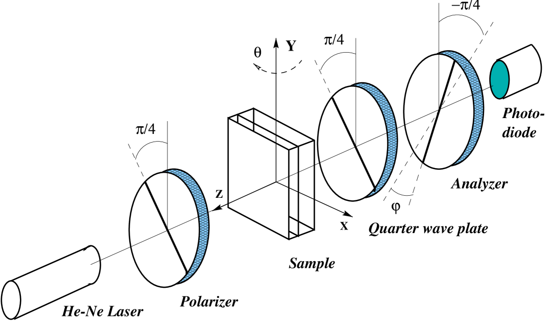
Figure 1: Experimental setup for the null ellipsometry measurements.

2.2 Null ellipsometry method

Instead of the prism coupling methods commonly used for the estimation of principle refractive indices we applied null ellipsometry technique Azzam and Bashara (1977) dealing with birefringence components. By this means we have avoided some disadvantages of prism coupling method such as the problem of making optical contact between the prism and the polymer layer.

The optical scheme of our method is presented in Fig. 1. The polymer film is placed between crossed polarizer and analyzer and a quarter wave plate with the optic axes oriented parallel to the polarization direction of the polarizer. The elliptically polarized beam passed through the sample is transformed into the linearly polarized light by means of the quarter wave plate. The polarization plane of this light is turned with respect to the polarization direction of the polarizer. This rotation is related to the phase retardation acquired by the light beam after passing through the film under investigation. It can be compensated by rotating the analyzer to the angle $\phi$ that encodes information on the phase retardation.

This method used for the normal incidence of the testing light is known as the Senarmont technique. It is suitable for the in-plane birefringence measurements.

Using oblique incidence of the testing beam we have extended this method for estimation of both in-plane, $n_{y}-n_{x}$, and out-of-plane $n_{z}-n_{x}$ birefringence ($n_{x}$, $n_{y}$ and $n_{z}$ are the principle refractive indices of the film shown in Fig. 1). In this case, the angle $\phi$ depends on the in-plane retardation $(n_{y}-n_{x})d$, the out-of-plane retardation $(n_{z}-n_{x})d$ and the absolute value of a refractive index of the biaxial film, say, $n_{x}$.

We need to have the light coming out of the quarter wave plate almost linear polarized when the system analyzes the phase shift between two orthogonal eigenmodes of the sample. In our experimental setup this requirement can be met, when the $x$ axis, directed along the polarization vector of the actinic light, is oriented horizontally or vertically. Dependencies of the analyzer rotation angle $\phi$ on the incidence angle of the testing beam $\theta$ were measured for both vertical and horizontal orientation of the $x$ axis. The value of $n_{x}$ was measured with the Abbe refractometer independently.

By using Berreman’s $4\times 4$ matrix method Berreman (1972), the $\theta$-dependencies of $\phi$ were calculated. Maxwell’s equations for the light propagation through the system of polarizer, sample and quarter wave plate were solved numerically for the different configurations of optical axes in the samples. The measured and computed $\phi$ versus $\theta$ curves were fitted in the most probable configuration model using the measured value of $n_{x}$.

We conclude on alignment of the azobenzene fragments from the obtained values of $(n_{y}-n_{x})d$ and $(n_{z}-n_{x})d$ assuming that the preferred direction of these fragments coincides with the direction of the largest refractive index. More details on the method can be found in our previous publication Yaroshchuk et al. (2001).

In our setup designed for the null ellipsometry measurements we used a low power He-Ne laser ($\lambda=632.8$ nm), two Glan-Thompson polarizers mounted on rotational stages from Oriel Corp., a quarter wave plate from Edmund Scientific and a sample holder mounted on the rotational stage. The light intensity was measured with a photodiode. The setup was automatically controlled by a personal computer. The rotation accuracy of the analyzer was better than 0.2 degree.

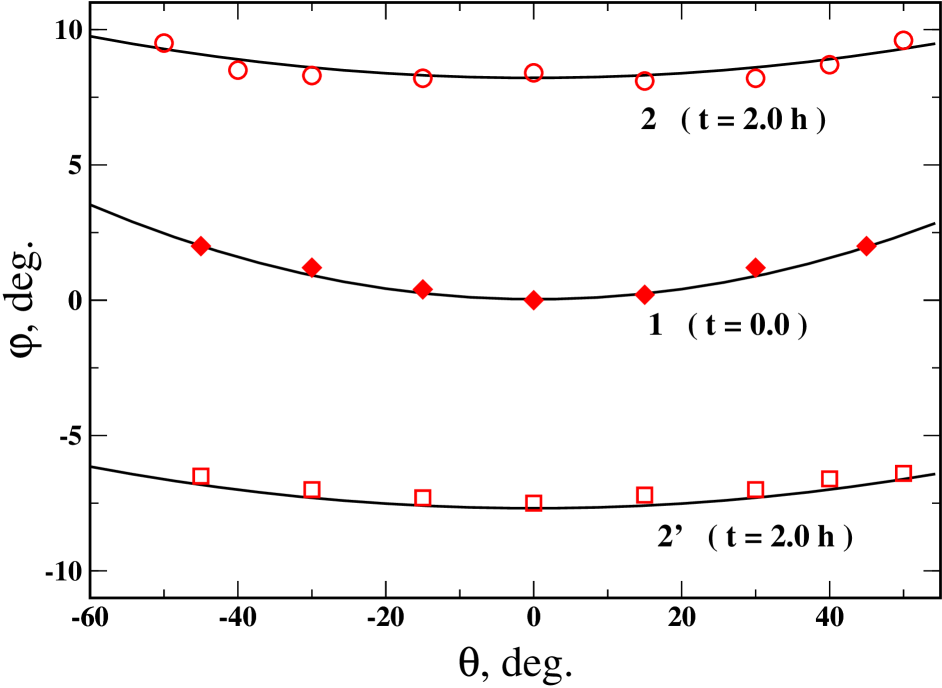
Figure 2: Dependencies of the phase shift $\phi$ on the incidence angle $\theta$ measured before (curve 1) and after irradiation (curves 2 and 2’).

2.3 Absorption measurements

The UV/Vis absorption measurements were carried out using a diode array spectrometer (Polytec XDAP V2.3). The samples were set normally to the testing beam of a deuterium lamp. A Glan-Thompson prism with a computer-driven stepper was used for polarization of the testing beam. The UV spectra of the original as well as irradiated films were measured in the spectral range of 220–400 nm with the rotation step of polarizer of 5 degree.

From these measurements the optical density components corresponding to the absorption maximum of azobenzene chromophores were estimated for the polarization direction of the testing light parallel to $x$ and $y$ axes, respectively. We denote them as $D_{x}$ and $D_{y}$, respectively. The out-of-plane component, $D_{z}$, was estimated by making use the method proposed in Wiesner et al. (1992); Phaadt et al. (1996). The latter assumes that the sample has uniaxial structure with in-plane position of the axis of anisotropy at the instant of time $t_{0}$. It implies that $D_{z}(t_{0})=D_{x}(t_{0})$ and the total absorption can be estimated as follows

$$D_{\mathrm{t}otal}=D_{x}(t_{0})+D_{y}(t_{0}) +D_{z}(t_{0})=$$

$$=2D_{x}(t_{0})+D_{y}(t_{0})\,.$$ (1)

When the number of trans azobenzene units does not change considerably, the total absorption is constant and the value of $D_{z}$ at instant of time $t$ can be determined from the following equation:

$$D_{z}(t)=D_{\mathrm{t}otal}-D_{x}(t)-D_{y}(t)\,,$$ (2)

where $D_{x}(t)$ and $D_{y}(t)$ are the experimentally measured parameters.

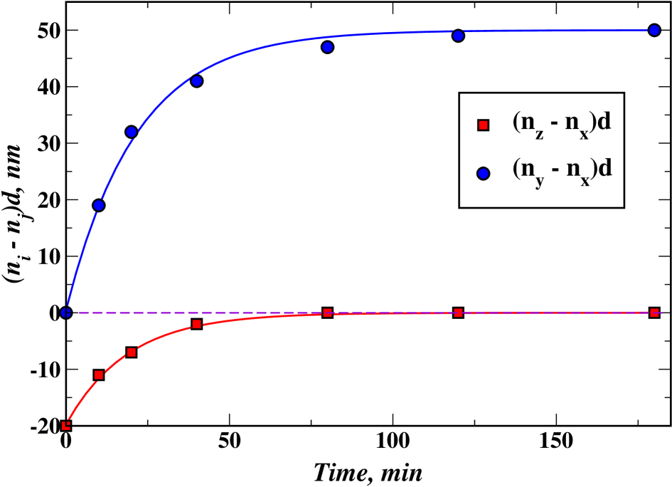
Figure 3: In-plane and out-of-plane birefringence as a function of the irradiation time.

2.4 Experimental results

Figure 2 shows the phase shift $\phi$ versus the incidence angle $\theta$ curve measured with null ellipsometry method for the non-irradiated polymer film. The curves $\phi(\theta)$ measured for vertical and horizontal position of $x$ axis overlaps. In addition, it is seen that there is no phase shift for normal light incidence ($\theta=0$). So we arrive at the conclusion that the in-plane indices are matched: $n_{y}=n_{x}$. The film, however, possesses out of plane birefringence $(n_{z}-n_{x})d=-20$ nm that results in a phase shift at oblique light incidence.

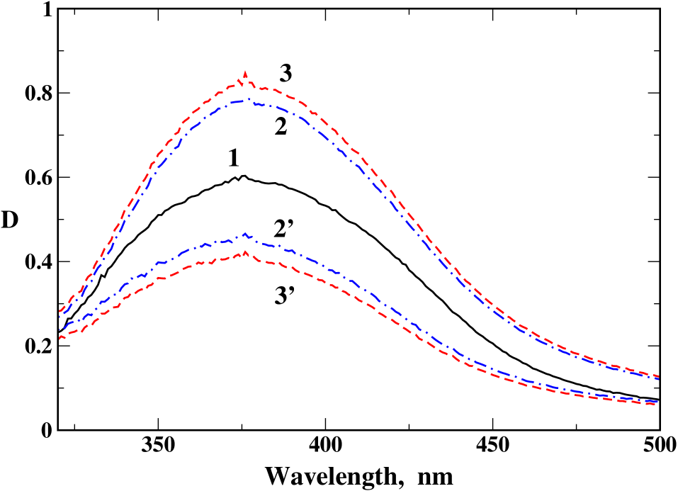
Figure 4: UV absorption spectra measured before (curve 1) and immediately after the irradiation over 1 h (curves 2 and 2’). The stationary spectra $D_{x}$ and $D_{y}$ (the waiting time is 15 min) are shown as the curves 3 and 3’, respectively.

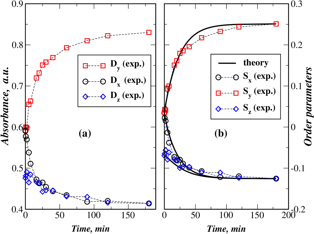
Figure 5: Dependencies of (a) the principle absorption coefficients and (b) the order parameter components on the irradiation time. Theoretical curves for the diagonal components of the order parameter tensor are shown as solid lines.

The fitting gives the following relations for the principle refractive indices: $n_{z}<n_{x}=n_{y}$ and $n_{z}-n_{x}\approx-0.1$. The film, therefore, demonstrates negative birefringence with the optical axis normal to the film surface. The relationship between the three indices suggests that the azobenzene fragments are randomly distributed in the plane of the film with no preferred direction for their orientation (a degenerate in-plane distribution).

Figure 2 shows the measured $\phi$ versus $\theta$ curves for the same polymer film after 2 h of UV light irradiation. Curves 1 and 2 correspond to vertical and horizontal position of the film $x$ axis, respectively.

According to the modeling, positive phase shift corresponds to the axis in the horizontal direction having the higher in-plane refractive index $n_{y}$ perpendicular to UV light polarization and the lower in-plane index $n_{x}$. From the curve fitting we have: $n_{y}-n_{x}=0.25$ ($(n_{y}-n_{x})d\approx 50nm$), $(n_{z}-n_{x})d=0$ nm, $n_{y}>n_{x}=n_{z}$. The light induced structure is positive uniaxial with the optical axis perpendicular to the UV light polarization. In this case, the azobenzene fragments show planar alignment perpendicular to the UV light polarization.

The fitted values of the in-plane, $n_{y}-n_{x}$, and out-of-plane birefringence, $n_{z}-n_{x}$, for various irradiation times are presented in Fig. 3. For small irradiation doses the principle refractive indices are different: $n_{z}<n_{x}<n_{y}$. The in-plane birefringence monotonously increases up to the saturated value with the increase of irradiation time. On the other hand, the difference between $n_{x}$ and $n_{z}$ decreases and becomes negligible in the photosaturated state. So the film is biaxial at the intermediate stages of irradiation, whereas the photosaturated state can be characterized as an uniaxial structure. The optical axis of this structure lies in the plane of the film and is directed along the $y$ axis.

The null ellipsometry identifies general orientational structure, but it does not provide the means to estimate the order parameters of various molecular groups. Different absorption methods are common for this purpose. In this case the wavelength of testing light is tuned to the absorption maximum of the selected molecular fragments.

In order to estimate the order parameter of azobenzene units we carried out UV absorption measurements in the absorption maximum of azobenzene chromophores. The UV/Vis spectrum of the studied azopolymer is presented in Fig. 4 (curve 1). It contains the intensive absorption band with the maximum at $\lambda=377$ nm corresponding to the $\pi\pi^{*}$ transition of trans azobenzene fragments.

The spectrum reveals polarization splitting during irradiation with polarized light. The polarization components $D_{x}$ and $D_{y}$, measured just after switching off the actinic light, are depicted in Fig. 4 as 2 and 2’, respectively. These spectra show changes that become stationary for approximately 10 min.

The stationary spectra $D_{x}$ and $D_{y}$ are shown in Fig. 4 as curves 3 and 3’, respectively. In order to have the azobenzene units relaxed to the stationary state, the components $D_{x}$ and $D_{y}$ were measured in 15 min after each irradiation period.

The experimentally measured absorption components $D_{x}$ and $D_{y}$ before irradiation and for different irradiation doses are presented in Fig. 5a. Kinetics of $D_{x}$ and $D_{y}$ is typical for reorientation mechanism of azobenzene units Dumont et al. (1993). Both curves reveal saturation. As it was shown by the null ellipsometry method, the saturated state of the polymer film under consideration is uniaxial with the in-plane orientation of the anisotropy axis.

In order to prove that the method described in Sect. 2.3 can be applied to estimate $D_{z}$, we need to show that, as compared to the non-irradiated film, the number of trans isomers does not change in the state relaxed after the irradiation. This is the case under the lifetime of cis isomers is shorter than the time of spectral relaxation after switching off the actinic light.

In order to estimate the lifetime of cis isomers we have measured relaxation of the spectral changes at $\lambda_{t}=377$ nm after irradiation with non-polarized light. Incidence directions of both actinic and testing light were approximately normal to the film. It was found that the relaxation curve $D(t)$ contains two components with characteristic times of 1.0 sec and 4 min, respectively. The first value can be attributed to cis-trans transition of azobenzene chromophores. The other time can be related to either the small fraction of long living cis isomers or more likely to the orientational relaxation of the azobenzene units. In any case, the waiting time of 15 min ensures that we definitely have all the cis isomers transformed into the trans form.

So in our measurements the concentration of trans isomers is preserved and the method described in Sect. 2.3 can be applied. The values of $D_{z}$ calculated for various irradiation doses using Eqs. (2.3)– (2) are presented in Fig. 5a. Dependencies $D_{x}(t)$, $D_{y}(t)$ and $D_{z}(t)$ show that the photoinduced ordering is mainly due to the in-plane reorientation of azobenzene fragments in the $y$ direction. In addition, slight reorientation in the $z$ direction is observed.

The orientational structure is generally described by the tensor $S_{ij}$, which is diagonal when the coordinate axes directed along the principle axes of the film. The diagonal elements $S_{xx}\equiv S_{x}$, $S_{yy}\equiv S_{y}$ and $S_{zz}\equiv S_{x}$ are related to the absorption components $D_{x}$, $D_{y}$ and $D_{z}$ Wiesner et al. (1992). For example,

$$S_{x}=\frac{2D_{x}-(D_{y}+D_{z})}{2(D_{x}+D_{y}+D_{z})}\,.$$ (3)

The components $S_{y}$ and $S_{z}$ can be obtained by the cyclic permutation in the expression (3).

The values of $S_{x}$, $S_{y}$ and $S_{z}$ calculated using equation (3) are presented in Fig. 5b. As is seen, during the initial stage of irradiation orientational configuration is biaxial, whereas the initial and the photosaturated states are uniaxial. These structures are characterized by the following order parameters: $S_{x}=S_{y}\approx 0.035$ and $S_{z}\approx-0.07$ for the non-irradiated film; $S_{x}=S_{z}\approx-0.1255$ and $S_{y}\approx 0.251$ for the film in the photosaturated state.

The transition between biaxial and uniaxial photoinduced orientations will be the subject of subsequent studies. We believe that a tendency to form an uniaxial structure is related to an intrinsic property of self-organization of mesogenic groups. Theoretically, similar tendency of nematic liquid crystals can be related to some specific features of the phase transition reflected in the form of the mean field free energy Patashinskii and Pokrovskii (1982). In this connection we assume that the irradiation with polarized light causes both the photoorientation of azochromophores and the self-aggregation as it was found for other liquid crystalline azopolymers Fisher et al. (1997a, b).

3 Theory

Before we proceed with theoretical considerations let us emphasize the following distinguishing features of POA in liquid crystalline azopolymers:

1. in contrast with the reversible POA, considered in Todorov et al. (1983); Dumont and Sekkart (1992, 1993); Dumont (1996); Neporent and Stolbova (1963), where POA disappears after switching off the irradiation, POA in liquid crystalline azopolymers can only be thermally erased by heating above clearing temperature. The long term stability of POA is caused by the photoorientation of the azobenzene;

2. the biaxiality effects discussed in Sect. 1.

Clearly, we can conclude that the photoorientation is a non-equilibrium process in a rather complex polymer system and it still remains a challenge to develop a tractable theory treating all the above points adequately.

As far as the long term stability of POA is concerned, the reorientation of the azobenzene groups can be assumed to result in the appearance of a self-consistent anisotropic field that support induced anisotropy. This field comes from anisotropic interactions between the azobenzene fragments and rearrangement of the main chains and other non-absorbing fragments. In other words, the photoinduced orientational structures can be regarded as a result of the photo-reorientation and thermotropic self-organization processes Fisher et al. (1997a).

There are two phenomenological models based on similar assumptions: the multidomain model proposed in Pederson and Michael (1997) and the model with additional order parameter, attributed to the polymer backbone and introduced to make the steady state degenerate Puchkovs’ka et al. (1998).

Despite these models look different it is clear that they incorporate the long term stability by introducing additional degree of freedom (subsystem) which kinetics would reflect cooperative motion and account for non-equilibrium behavior.

In this section we describe our theoretical approach to the kinetics of the photoinduced reorientation. We begin with the analysis of general master equations and specialize then the rates of the involved transitions. The resulting kinetic equations for order parameters are derived after making assumptions on the form of angular redistribution probabilities and the order parameter correlation functions. In addition, we show that this approach can be employed to derive the known phenomenological models Pederson and Michael (1997); Puchkovs’ka et al. (1998); Yaroshchuk et al. (1999a). Finally at the end of the section we present the numerical results obtained by solving the kinetic equations for the order parameters and concentrations.

3.1 Master equations

We shall assume that the dye molecules in the ground state are of trans form with the orientation of the molecular axis defined by the unit vector $\mathbf{\hat{n}}$. The latter is specified by the polar, $\theta$, and azimuthal, $\phi$, angles: $\mathbf{\hat{n}}=$($\sin\theta\cos\phi$,$\sin\theta\sin\phi$, $\cos\theta$).

Angular distribution of the trans molecules at time $t$ is characterized by the number distribution function $N_{tr}(\mathbf{\hat{n}},t)$. Molecules in the excited state have the cis conformation and the corresponding function is $N_{cis}(\mathbf{\hat{n}},t)$. Then for the number of trans and cis molecules we have

$$N_{tr}(t)\equiv Nn_{tr}(t)=\int N_{tr}(\mathbf{\hat{n}},t)\,\mathrm{d}\mathbf{\hat{n}},$$ (4)

$$N_{cis}(t)\equiv Nn_{cis}(t)=\int N_{cis}(\mathbf{\hat{n}},t)\,\mathrm{d}\mathbf{\hat{n}},$$ (5)

$$N=N_{tr}(t)+N_{cis}(t)\,,\qquad n_{tr}(t)+n_{cis}(t)=1\,,$$ (6)

where $\displaystyle\int\,\mathrm{d}\mathbf{\hat{n}}\equiv\int_{0}^{2\pi}\mathrm{d}\phi\int_{0}^{\pi}\,\sin\theta\,\mathrm{d}\theta\,$ and $N$ is the total number of molecules.

We shall refer the additional subsystem that is able to accumulate induced ordering of the side chain molecules as a polymer system (matrix). From the phenomenological point of view, this system can be thought to represent some collective degrees of freedom of non-absorbing units such as main chains. We shall suppose that it is characterized by the angular distribution function $f_{p}(\mathbf{\hat{n}},t)$, so that $N_{p}(\mathbf{\hat{n}},t)=N_{p}f_{p}(\mathbf{\hat{n}},t)$. Note that the coefficient $N_{p}$ can be considered as an effective number of the units related to the polymer system. But, more precisely, this factor determine the relations between different thermal relaxation constants (see Eq. (13)).

The starting point of our approach is the kinetic rate equations taken in the following general form van Kampen (1984); Gardiner (1985):

$$\frac{\partial N_{\alpha}}{\partial t} =\left[\frac{\mathrm{d}N_{\alpha}}{\mathrm{d}t}\right]_{\mathrm{Diff}}+\sum_{\beta\neq\alpha}\int\Bigl{[}\,W_{\alpha\leftarrow\beta}(\mathbf{\hat{n}},\mathbf{\hat{n}}^{\prime})\,N_{\beta}(\mathbf{\hat{n}}^{\prime},t)-$$

$$-W_{\beta\leftarrow\alpha}(\mathbf{\hat{n}}^{\prime},\mathbf{\hat{n}})\,N_{\alpha}(\mathbf{\hat{n}},t)\,\Bigr{]}\,\mathrm{d}\mathbf{\hat{n}}^{\prime}\,,\quad$$ (7)

where $\alpha\,,\beta\in\{tr,\,cis,\,p\}$.

The first term on the right hand side of Eq. (7) is due to rotational diffusion of molecules in trans ($\alpha=tr$) and cis ($\alpha=cis$) conformations. Note that the terms proportional to $W_{\alpha\leftarrow\alpha}$ can be incorporated into this diffusion term. In what follows it is supposed that

$$\left[\frac{\mathrm{d}N_{tr}}{\mathrm{d}t}\right]_{\mathrm{Diff}}=\left[\frac{\mathrm{d}f_{p}}{\mathrm{d}t}\right]_{\mathrm{Diff}}=0\,.$$ (8)

Now in order to proceed we need to specify the rates of the transitions.

3.2 Transition rates

The trans–cis transition is stimulated by the incident UV–light quasiresonant to the transition. Assuming that the electromagnetic wave is linearly polarized along the $x$–axis, the transition rate can be written as follows Dumont and Sekkart (1992); Dumont (1996):

$$W_{cis\leftarrow tr}(\mathbf{\hat{n}},\mathbf{\hat{n}}^{\prime})=\Gamma_{c-t}(\mathbf{\hat{n}},\mathbf{\hat{n}}^{\prime})\,P_{tr}(\mathbf{\hat{n}}^{\prime}),$$

$$\int\Gamma_{c-t}(\mathbf{\hat{n}},\mathbf{\hat{n}}^{\prime})\,\mathrm{d}\mathbf{\hat{n}}=1\,,$$ (9)

$$\begin{aligned} P_{tr}(\mathbf{\hat{n}}^{\prime})&=(\hbar\omega_{t})^{-1}\Phi_{tr\to cis}\sum_{i,j}\sigma_{ij}^{(tr)}(\mathbf{\hat{n}}^{\prime})E_{i}E_{j}^{*}=\\ &=q_{t}I(1+u\,n_{x}^{2})\equiv q_{t}I(1+u\,(2S_{x}+1)/3)\,,\end{aligned}$$

where $\boldsymbol{\sigma}^{(tr)}(\mathbf{\hat{n}})$ is the tensor of absorption cross section for the trans molecule oriented along $\mathbf{\hat{n}}$: ${\sigma}^{(tr)}_{ij}=\sigma_{\perp}^{(tr)}\delta_{ij}+(\sigma_{||}^{(tr)}-\sigma_{\perp}^{(tr)})\,n_{i}\,n_{j}$; $u\equiv(\sigma_{||}^{(tr)}-\sigma_{\perp}^{(tr)})/\sigma_{\perp}^{(tr)}$ is the absorption anisotropy parameter; $\hbar\omega_{t}$ is the photon energy; $\Phi_{tr\to cis}$ is the quantum yield of the process and $\Gamma_{tr}(\mathbf{\hat{n}},\mathbf{\hat{n}}^{\prime})$ describes the angular redistribution of the molecules excited in the cis state; $I$ is the pumping intensity.

Similar line of reasoning applies to the cis–trans transition, so we have

$$W_{tr\leftarrow cis}(\mathbf{\hat{n}},\mathbf{\hat{n}}^{\prime})=\gamma_{c}\Gamma_{t-c}^{(sp)}(\mathbf{\hat{n}},\mathbf{\hat{n}}^{\prime})+q_{c}I\,\Gamma_{t-c}^{(ind)\,}(\mathbf{\hat{n}},\mathbf{\hat{n}}^{\prime}),$$

$$q_{c}\equiv\Phi_{cis\to trans}\sigma^{(cis)}\,,$$ (10)

where $\gamma_{c}\equiv 1/\tau_{c}$, $\tau_{c}$ is the lifetime of cis molecule and the anisotropic part of the absorption cross section is disregarded, $\sigma_{||}^{(cis)}=\sigma_{\perp}^{(cis)}\equiv\sigma^{(cis)}$. Eq. (3.2) implies that the process of angular redistribution for induced and spontaneous transitions can differ. Note that the normalization condition for all the angular redistribution probability intensities is

$$\int\Gamma_{\alpha-\beta}(\mathbf{\hat{n}},\mathbf{\hat{n}}^{\prime})\,\mathrm{d}\mathbf{\hat{n}}=1\,.$$ (11)

The remaining part of transitions describes equilibrating between the side chain absorbing molecules and the polymer system. The corresponding rates can be taken in the form:

$$W_{\alpha\leftarrow p}(\mathbf{\hat{n}},\mathbf{\hat{n}}^{\prime})=\gamma_{\alpha-p}\Gamma_{\alpha-p}(\mathbf{\hat{n}},\mathbf{\hat{n}}^{\prime}),$$

$$W_{p\leftarrow\alpha}(\mathbf{\hat{n}},\mathbf{\hat{n}}^{\prime})=\gamma_{p-\alpha}\Gamma_{p-\alpha}(\mathbf{\hat{n}},\mathbf{\hat{n}}^{\prime}),\quad\alpha\in\{tr,\,cis\}\,,$$ (12)

where $\gamma_{\alpha-p}$ and $\gamma_{\alpha-p}$ are angular independent. In addition, since thermal relaxation does not change the number of molecules in a particular state we have the relation for $\gamma_{\alpha-p}$ and $\gamma_{p-\alpha}$:

$$N_{p}\gamma_{\alpha-p}=Nn_{\alpha}\gamma_{p-\alpha}\,.$$ (13)

As it was mentioned above, this equation relates the thermal relaxation constants of the polymer and the fragments through the coefficient $N_{p}$, introduced in Sect. 3.1.

3.3 Model

At this stage it is convenient to introduce normalized angular distribution functions, $f_{\alpha}(\mathbf{\hat{n}},t)$:

$$N_{\alpha}(\mathbf{\hat{n}},t)=Nn_{\alpha}(t)f_{\alpha}(\mathbf{\hat{n}},t)\,.$$ (14)

From Eqs. (7), (9) and (3.2) it is not difficult to obtain equation for $n_{tr}(t)$:

$$\frac{\partial n_{tr}(t)}{\partial t}=(\gamma_{c}+q_{c}I)\,n_{cis}(t)-\langle P_{tr}\rangle_{tr}n_{tr}(t)\,,$$ (15)

where the angular brackets $\langle\ldots\rangle_{\alpha}$ stand for averaging over angles with the distribution function $f_{\alpha}$ . Owing to the condition (11), this equation does not depend on the form of the angular redistribution probabilities.

From the results of the previous section and Eq. (15) we derive the equations for the distribution functions

$$n_{cis}(t)\,\frac{\partial f_{cis}(\mathbf{\hat{n}},t)}{\partial t}=n_{cis}(t)\Biggl{\{}\left[\frac{\mathrm{d}f_{cis}}{\mathrm{d}t}\right]_{\mathrm{Diff}}-$$

$$-\gamma_{cis}\,f_{cis}(\mathbf{\hat{n}},t)\Biggr{\}}-\langle P_{tr}\rangle_{tr}n_{tr}(t)+$$

$$+n_{tr}(t)\int\Gamma_{c-t}(\mathbf{\hat{n}},\mathbf{\hat{n}}^{\prime})P_{tr}(\mathbf{\hat{n}}^{\prime})f_{tr}(\mathbf{\hat{n}}^{\prime},t)\,\mathrm{d}\mathbf{\hat{n}}^{\prime}+$$

$$+\gamma_{cis}\,n_{cis}(t)\int\Gamma_{c-p}(\mathbf{\hat{n}},\mathbf{\hat{n}}^{\prime})f_{p}(\mathbf{\hat{n}}^{\prime},t)\,\mathrm{d}\mathbf{\hat{n}}^{\prime}\,,$$ (16)

$$n_{tr}(t)\,\frac{\partial f_{tr}(\mathbf{\hat{n}},t)}{\partial t}=-n_{tr}(t)\left[P_{tr}(\mathbf{\hat{n}})-\langle P_{tr}\rangle_{tr}+\gamma_{tr}\right]f_{tr}(\mathbf{\hat{n}},t)+$$

$$+\gamma_{c}\,n_{cis}(t)\int\Gamma_{t-c}^{(sp)}(\mathbf{\hat{n}},\mathbf{\hat{n}}^{\prime})f_{cis}(\mathbf{\hat{n}}^{\prime},t)\,\mathrm{d}\mathbf{\hat{n}}^{\prime}+$$

$$+q_{c}In_{cis}(t)\int\Gamma_{t-c}^{(ind)}(\mathbf{\hat{n}},\mathbf{\hat{n}}^{\prime})f_{cis}(\mathbf{\hat{n}}^{\prime},t)\,\mathrm{d}\mathbf{\hat{n}}^{\prime}-$$

$$-(\gamma_{c}+q_{c}I)\,n_{cis}(t)\,f_{tr}(\mathbf{\hat{n}},t)+$$

$$+\gamma_{tr}\,n_{tr}(t)\int\Gamma_{t-p}(\mathbf{\hat{n}},\mathbf{\hat{n}}^{\prime})f_{p}(\mathbf{\hat{n}}^{\prime},t)\,\mathrm{d}\mathbf{\hat{n}}^{\prime}\,,$$ (17)

$$\frac{\partial f_{p}(\mathbf{\hat{n}},t)}{\partial t}=-\gamma_{p}^{(tr)}\,n_{tr}(t)\Biggl{(}f_{p}(\mathbf{\hat{n}},t)-$$

$$-\int\Gamma_{p-t}(\mathbf{\hat{n}},\mathbf{\hat{n}}^{\prime})f_{tr}(\mathbf{\hat{n}}^{\prime},t)\,\mathrm{d}\mathbf{\hat{n}}^{\prime}\Biggr{)}-\gamma_{p}^{(cis)}\,n_{cis}(t)\Biggl{(}f_{p}(\mathbf{\hat{n}},t)-$$

$$-\int\Gamma_{p-c}(\mathbf{\hat{n}},\mathbf{\hat{n}}^{\prime})f_{cis}(\mathbf{\hat{n}}^{\prime},t)\,\mathrm{d}\mathbf{\hat{n}}^{\prime}\Biggr{)}\,,$$ (18)

where $\gamma_{tr}\equiv\gamma_{p-trans}$, $\gamma_{cis}\equiv\gamma_{p-cis}$ and $\gamma_{p}^{(\alpha)}\equiv N\gamma_{\alpha}/N_{p}$. These equations supplemented with Eq. (15) are derived on the basis of quite general considerations. They can be regarded as a starting point for the formulation of a number of phenomenological models. We can now describe our model.

Our basic assumptions of the angular redistribution operators $\Gamma_{\alpha-\beta}$ are as follows

$$\gamma_{cis}=0,\quad\Gamma_{t-c}^{(sp)}(\mathbf{\hat{n}},\mathbf{\hat{n}}^{\prime})=\Gamma_{t-p}(\mathbf{\hat{n}},\mathbf{\hat{n}}^{\prime})=$$

$$\phantom{\gamma_{cis}=0,\quad\Gamma_{t-c}^{(sp)}(\mathbf{\hat{n}},\mathbf{\hat{n}}^{\prime})}=\Gamma_{p-t}(\mathbf{\hat{n}},\mathbf{\hat{n}}^{\prime})=\delta(\mathbf{\hat{n}}-\mathbf{\hat{n}}^{\prime}),$$ (19)

$$\Gamma_{t-c}^{(ind)}(\mathbf{\hat{n}},\mathbf{\hat{n}}^{\prime})=f_{tr}(\mathbf{\hat{n}},t),\quad\Gamma_{c-t}(\mathbf{\hat{n}},\mathbf{\hat{n}}^{\prime})=f_{cis}(\mathbf{\hat{n}},t)\,.$$ (20)

It gives the resulting system of kinetic equations:

$$\frac{\partial f_{cis}}{\partial t}=\left[\frac{\mathrm{d}f_{cis}}{\mathrm{d}t}\right]_{\mathrm{Diff}}$$ (21a)

$$n_{tr}\frac{\partial f_{tr}}{\partial t}=\left(\langle P_{tr}\rangle_{tr}-P_{tr}-\gamma_{tr}\right)n_{tr}f_{tr}+$$

$$+\gamma_{c}\,n_{cis}\,(\,f_{cis}-f_{tr}\,)+\gamma_{tr}\,n_{tr}\,f_{p}\,,$$ (21b)

$$\frac{\partial f_{p}}{\partial t}=\gamma_{p}\,n_{tr}(f_{tr}-f_{p})\,,$$ (21c)

where $\gamma_{p}\equiv\gamma_{p}^{(tr)}$.

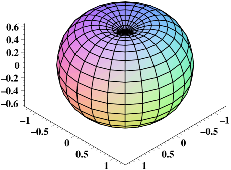
(a) $t=0.0$ min

(b) $t=10.0$ min

(c) $t=120.0$ min

Figure 6: The orientational distribution functions of trans molecules at different illumination doses. These surfaces are defined by the equation: $r(\theta.\phi)=4\pi\,n_{tr}(t)\,f_{tr}(\theta,\phi,t)$ in the spherical coordinate system at irradiation time $t$.

Clearly, the meaning of Eq. (19) is that the molecules do not change orientation under spontaneous transitions. On the other hand, from Eq. (20) projecting onto the angular distribution function of the corresponding state describes angular redistribution for the stimulated transitions.

In order to explain the meaning of the projectors, note that the multidomain model considered in Pederson and Michael (1997) can be derived from Eqs. (16) – (18) by putting $\gamma_{c}=0$, $\gamma_{cis}=\gamma_{tr}$ and assuming that all angular redistribution probabilities are equal to the equilibrium distribution, $\Gamma_{\alpha-\beta}(\mathbf{\hat{n}},\mathbf{\hat{n}}^{\prime})=p(\mathbf{\hat{n}})$, determined by the mean field potential $W(\mathbf{\hat{n}})$: $p(\mathbf{\hat{n}})\propto\exp(-W)$. In other words, this procedure introduces the mean field potential by assuming that the angular redistribution operators $\Gamma_{\alpha-\beta}$ act as projectors onto the equilibrium distribution. Note that the results of Puchkovs’ka et al. (1998); Yaroshchuk et al. (1999a) correspond to the case where $\Gamma_{t-c}^{(sp)}(\mathbf{\hat{n}},\mathbf{\hat{n}}^{\prime})=f_{tr}(\mathbf{\hat{n}},t)$ and $\Gamma_{t-c}^{(ind)}(\mathbf{\hat{n}},\mathbf{\hat{n}}^{\prime})=(4\pi)^{-1}$.

3.4 Order parameters

We can now deduce the equations that describe the temporal evolution of the diagonal components of the order parameter tensor

$$\mathbf{S}(\mathbf{\hat{n}})=2^{-1}\,(3n_{i}n_{j}-\delta_{ij})\,\mathbf{\hat{e}}_{i}\otimes\mathbf{\hat{e}}_{j}\,.$$ (22)

The components of interest can be expressed in terms of Wigner $D$–functions Biedenharn and Louck (1981) as follows

$$S_{x}=(3n_{x}^{2}-1)/2=$$

$$\phantom{S_{x}}=-(D_{00}^{2}(\mathbf{\hat{n}})-\sqrt{6}\,\mathop{\rm Re}\nolimits D_{20}^{2}(\mathbf{\hat{n}}))/2\,,$$ (23)

$$S_{y}=(3n_{y}^{2}-1)/2=$$

$$\phantom{S_{y}}-(D_{00}^{2}(\mathbf{\hat{n}})+\sqrt{6}\,\mathop{\rm Re}\nolimits D_{20}^{2}(\mathbf{\hat{n}}))/2\,,$$ (24)

$$S_{z}=(3n_{z}^{2}-1)/2=D_{00}^{2}(\mathbf{\hat{n}})\,.$$ (25)

The simplest case occurs for the order parameters of cis molecules. Eq. (21a) yields the following result:

$$\frac{\partial S_{ij}^{(cis)}}{\partial t}=-6D_{r}S_{ij}^{(cis)}\,,$$ (26)

where $S_{ij}^{(\alpha)}\equiv\langle S_{ij}(\mathbf{\hat{n}})\rangle_{\alpha}$ and $D_{r}$ is the rotational diffusion constant. Clearly, our assumptions correspond to the case where the presence of cis molecules is of minor importance for ordering kinetics.

Eqs. (3.2), (21b) and (21c) give the following system for the components of the order parameter tensor:

$$n_{tr}\frac{\partial S_{ij}^{(tr)}}{\partial t}=-2/3\,q_{t}Iu\,n_{tr}\,G_{ij;\,xx}^{(tr)}+$$

$$+\gamma_{c}n_{cis}(S_{ij}^{(cis)}-S_{ij}^{(tr)})+\gamma_{tr}n_{tr}(S_{ij}^{(p)}-S_{ij}^{(tr)})\,,$$ (27a)

$$\frac{\partial S_{ij}^{(p)}}{\partial t}=-\gamma_{p}n_{tr}(S_{ij}^{(p)}-S_{ij}^{(tr)})\,,$$ (27b)

where $G_{ij;\,mn}^{(\alpha)}$ is the correlation function of the order parameter components $S_{ij}(\mathbf{\hat{n}})$ and $S_{mn}(\mathbf{\hat{n}})$ that is defined by the following relation

$$G_{ij;\,mn}^{(\alpha)}=\langle S_{ij}(\mathbf{\hat{n}})S_{mn}(\mathbf{\hat{n}})\rangle_{\alpha}-S_{ij}^{(\alpha)}\,S_{mn}^{(\alpha)}\,.$$ (28)

Computing the order parameter correlation functions that enter Eqs. (27) requires the knowledge of details on microscopic interactions and, in general, for nonequilibrium system it can be rather involved and sophisticated. In this paper, we shall adopt the simplest “kinematic” procedure to approximate the correlators. It implies that after writing the products of $D$–functions as a sum of spherical harmonics we neglect the high order harmonics with angular momentum $j>2$. In particular, we have

$$\langle S_{\alpha}^{2}\rangle_{tr}\approx 1/5+2/7\,\langle S_{\alpha}\rangle_{tr}\,,\quad\alpha\in\{x,\,y,\,z\}\,.$$ (29)

Applying this procedure to Eqs. (27) leads to the result given by

$$n_{tr}\frac{\partial S}{\partial t}=2u/3\,q_{t}I(1/5+2/7\,S-S^{2})n_{tr}-$$

$$-\gamma_{c}n_{cis}S++\gamma_{tr}n_{tr}(S_{p}-S)\,,$$ (30)

$$n_{tr}\frac{\partial\Delta S}{\partial t}=-2u/3\,q_{t}I(2/7+S)n_{tr}\Delta S-$$

$$-\gamma_{c}n_{cis}\Delta S+\gamma_{tr}n_{tr}(\Delta S_{p}-\Delta S)\,,$$ (31)

$$\frac{\partial S_{p}}{\partial t}=-\gamma_{p}n_{tr}(S_{p}-S)\,,$$ (32)

$$\frac{\partial\Delta S_{p}}{\partial t}=-\gamma_{p}n_{tr}(\Delta S_{p}-\Delta S)\,,$$ (33)

where $S\equiv\langle S_{y}\rangle_{tr}$, $\Delta S\equiv\langle S_{x}-S_{z}\rangle_{tr}$, $S_{p}\equiv\langle S_{y}\rangle_{p}$ and $\Delta S_{p}\equiv\langle S_{x}-S_{z}\rangle_{p}$. Eqs. (30) – (33) combined with Eq. (15) form the system of kinetic equations for our phenomenological model.

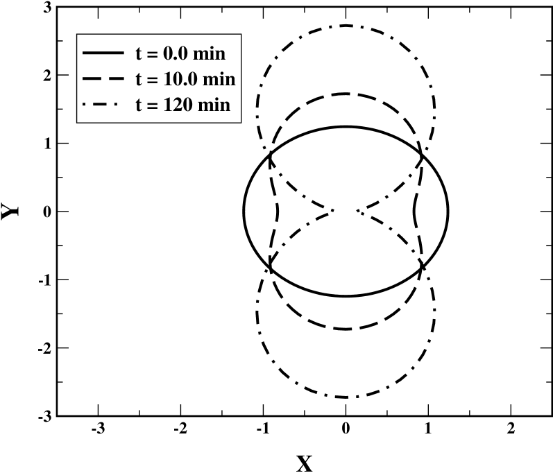
Figure 7: Initial orientational distribution at section by the $x$-$y$ plane is isotropic. It assumes anisotropy along the $y$ axis as illumination time increases.

3.5 Numerical results

Theoretical curves depicted in Fig. 5b are calculated by solving the equations deduced in the previous section. This procedure involves computing the stationary values of $S$ and $\Delta S$ to which the order parameters decays after switching off the irradiation at time $t$. In addition, we need to take into consideration the difference between the order parameters defined by Eq. (3) and the order parameters of Sect. 3.4. Since $D_{i}\propto(1+u(2\,S_{i}+1)/3)$, these order parameters differ by the factor $u/(3+u)$.

According to the experimental data, the lifetime of cis molecules $\tau_{c}$ ($\gamma_{c}=1/\tau_{c}$) is about 1.0 sec, whereas the relaxation time after switching off the irradiation can be estimated at 4 min. Since the theoretical value of this relaxation time is $1/(\gamma_{p}+\gamma_{tr})$, the relaxation times $\tau_{p}$ ($\gamma_{p}=1/\tau_{p}$) and $\tau_{tr}$ ($\gamma_{tr}=1/\tau_{tr}$) can be taken to be equal 8 min.

We estimated the absorption cross sections $\sigma^{(cis)}$ and $\sigma^{(tr)}$ from the UV spectra of the polymer solved in toluene. These spectra were measured before and during irradiation. In the latter case the solution was in the photosaturated state. The absorption bands were then decomposed into the bands of trans and cis isomers to yield the corresponding values of the extinction coefficients at $\lambda_{t}=365$ nm. In order to compute these coefficients we followed the procedure described in Bernstein and Kaminskii (1975). The resulting estimates can be written as follows: $(\hbar\omega_{t})^{-1}\sigma^{(cis)}\tau_{c}I\approx 0.2\times 10^{-2}$ and $\sigma^{(tr)}/\sigma^{(cis)}\approx 2.5$ for $I=1$ mW/cm², where $\sigma^{(tr)}=(\sigma_{||}^{(tr)}+2\sigma_{\perp}^{(tr)})/3$ is the average absorption cross section of the trans fragments.

Then given the quantum yield $\Phi_{cis\to trans}$ and the experimental value of the order parameter in the photosteady state, $S_{st}=0.251\,(1+3/u)$, we can compute the anisotropy parameter $u$ from the equation for $S_{st}$. The latter can be derived from Eqs. (15) and (30) by setting the time derivatives on the left hand sides equal to zero:

$$\gamma_{c}S_{st} (1+u(1-S_{st})/3)=$$

$$=2u/3\,(\gamma_{c}+q_{c}I)\,(1/5\,+2/7\,S_{st}-S_{st}^{\,2})\,.$$ (34)

The theoretical curves in Fig. 5b are calculated at $\Phi_{cis\to trans}=10$% and $\Phi_{cis\to trans}=5$% that is to yield the value of the ratio $\sigma_{||}^{(tr)}/\sigma_{\perp}^{(tr)}=8.9$. Note that the quantum efficiencies are of the same order of magnitude as the experimental values for other azobenzene compounds Mita et al. (1989). On the other hand, we have $q_{c}\approx 0.2\times 10^{-3}$ cm²/mJ that is about the value given in Pederson and Michael (1997).

The computed order parameter components can be used to illustrate orientational distributions of trans fragments maintained after different illumination doses. Fig. 6 shows the surfaces $r(\theta.\phi)=4\pi\,n_{tr}(t)\,f_{tr}(\theta,\phi,t)$ that indicate the angular redistribution in the course of irradiation. Note that we have truncated the expansion for the distribution function $f_{tr}$ by neglecting the high order spherical harmonics:

$$4\pi\,f_{tr}(\mathbf{\hat{n}},t)\approx 1+5\,\Bigl{[}\langle S_{z}\rangle_{tr}D^{\,2}_{00}(\mathbf{\hat{n}})+$$

$$+\frac{\langle S_{x}\rangle_{tr}-\langle S_{y}\rangle_{tr}}{\sqrt{6}}\,2\,\mathop{\rm Re}\nolimits D^{\,2}_{20}(\mathbf{\hat{n}})\Bigr{]}\,.$$ (35)

Sections of the surfaces depicted in Fig. 6 by the $x$-$y$ and $x$-$z$ coordinate planes are shown in Figs. 7 – 8. As is seen from Fig. 7, the angular distribution in the $x$-$y$ plane becomes anisotropic under the action of light, whereas Fig. 8 indicates that the distribution in the $x$-$z$ plane goes isotropic.

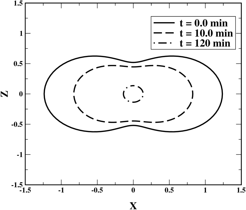
Figure 8: Increase in the illumination dose renders the orientational distribution of the trans fragments at section by the $x$-$z$ plane isotropic.

4 Conclusions

In this paper we demonstrate that the combination of the UV/Vis absorption spectroscopy and the suitably modified null ellipsometry method is a tool appropriate for a comprehensive study of POA in films of liquid crystalline polymers with azobenzene side groups.

We found that initially the spincoated films under investigation are characterized by a preferred in-plane orientation of the azobenzene fragments, whereas the long axes are randomly distributed in this plane. So, the resulting structure is isotropic in this plane, but in the space it is uniaxial with the optical axis normal to the film surface resulting in a negative birefringence (see Sect. 2.4).

Increasing irradiation doses results in an anisotropic order maintained in the film after switching off the linearly polarized UV light. This photo-induced structure corresponds to a biaxial orientational order of the azobenzene moieties. But it becomes uniaxial at sufficiently large doses reaching the photosaturated state of the photoorientation process. The process results usually in an oblate order in the case of amorphous polymers. The uniaxiality in the studied case could be related to liquid crystalline character of the polymer or the initial order of the film which act in combination with the linearly polarized light as aligning force resulting in an uniaxial in-plane order. So, the action of the actinic light can be regarded as a factor stimulating both photoorientation and thermotropic self-organization.

Quantitatively, experimental results on the kinetics of the photoreorientation were described in terms of the order parameters introduced in Sect. 2.4. It makes the comparison between experimental and theoretical results relatively direct. On the other hand, it raises the question as to the validity of the procedure used to determine the out-of-plane absorption $D_{z}$. In our case this can be justified for the number of trans fragments is shown to remain unchanged in all the relaxed states caused by the lifetime of cis isomer. So, the conclusion is that the photoreorientation in the film occurs through the mechanism of angular redistribution. Note that, as a matter of fact, the latter was implicitly assumed in our theoretical model formulated in Sect. 3.3.

Despite the theoretical considerations of Sect. 3 are rather phenomenological they emphasize the key points that should be addressed by such kind of theories. These are the angular redistribution probabilities (Sect. 3.3) and the order parameter correlation functions (Sect. 3.4). The redistribution operators, in particular, define how the system relaxes after switching off the irradiation and can serve to introduce self-consistent fields. The correlators, roughly speaking, mainly determine the character of photoreorientation and the properties of the photosaturated state.

The assumptions taken in this paper give the model with the kinetics governed by the mechanism of angular redistribution. The form of the approximate correlators influences it in such a way that the out-of-plane reorientation is appeared to be suppressed.

Our simple model depends on a few parameters that enter the equations and that can be estimated from the experimental data. Only the anisotropy parameter and the quantum yields are derived by making comparison between the experimental data and the theoretical dependencies.

This theory predicts that the fraction of cis isomers is negligible and the orientational kinetics of the cis fragments governed by Eq. (26) is irrelevant. The latter is why the liquid crystalline ordering effects Doi and Edwards (1986) that would complicate the kinetics of the cis molecules can be safely omitted in Eq. (26). Note, however, that it is rather straightforward to modify the model for the case where the cis fragments would affect the kinetics considerably. We shall extend on the subject elsewhere.

More detailed microscopic theoretical approach is apparently beyond the scope of the paper. Theoretically, it would be interesting to put this theory into the context of ergodicity breaking transitions Kiselev (2000). This work is under progress.