Representation of the short-range interactions in liquid helium via modified hard sphere potentials

Abstract

In this paper we propose five different modifications of the hard sphere potential for the modeling a short-range repulsion and the calculation of thermodynamic and transport properties of liquid ⁴He. We calculate the potential energy, the total energy, and the sound velocity at $T=0$ K. It is shown that three of the proposed potentials give a satisfactory description of these properties.

Keywords: liquid helium, interatomic potential, short-range interaction, thermodynamic properties, sound velocity.

PACS numbers: 34.20.Cf, 67.40.Kh, 67.40.Mj.

1 Introduction

In this paper we calculate some properties of the helium system using the modifications of helium–helium interatomic potential obtained in [2].

The method of receiving the potential is based on the collective variables formalism as described in our previous work [2].

Numerical methods could be grouped in two large parts: 1) calculations with adjustable parameters using experimental data on thermodynamic and transport properties [3, 4, 5, 6], 2) ab initio quantum-mechanical computations (mainly Monte Carlo) [7, 8]. A good comparison between various potentials, calculated properties of helium, and the experimental data might be found in [9].

We analyze our potentials due to the form of the potential curve and such properties as the potential energy, the total energy, and the sound velocity, all calculated at $T=0$ K, i. e., for the ground state.

Concerning the form of the potential curve, one can notice that the short-range part of the potential is not very significant starting from distances about 2 Å and less. This statement becomes clear if one looks at the pair distribution function $F_{2}(R)$ of helium [10]: $F_{2}(R<2.212{\rm~{}\AA})=0$.

On the other hand, the results for the potential from [2] lead to the value $-7.8$ K for the total energy of the system of helium atoms at 0 K, while the experiment gives $-7.17$ K [11], we consider it as a good agreement. But we obtained the value of the potential energy $-15.5$ K, and computer simulations [9] predict it in the range from about $-20$ to $-22$ K (there is no experimental measurements available for this quantity). This difference may not seem to be quite satisfactory if one calculates quantities connected with the potential energy only.

Thus, we tried to correct our potential for it could reflect the short-range interactions more precisely unlike that obtained in [2]. For this purpose we used some modification of the hard sphere potential.

The paper is organized as follows. The calculating procedure is described in the Section 2. Different forms for the short-range repulsion are presented in the Section 3, the respective potential curves are also given there. In the Section 4 we adduce the computation of the energy and the sound velocity of ⁴He in the ground state.

2 Calculating procedure

The following relation was used for the calculation of the potential Fourier image $\nu_{q}$. see [2, 12]:

$$\frac{N}{V}\frac{m\nu_{q}}{\hbar^{2}} + {\bf q}^{2}\,a_{2}({\bf q})-{\bf q}^{2}\,a_{2}^{2}({\bf q})-\frac{1}{2N}\sum_{\bf k\neq 0}{\bf k}^{2}\,a_{4}({\bf k,-k,q,-q})$$

$${}+\frac{1}{N}\sum_{\bf k\neq 0}{\bf k(-k-q)}\,a_{3}({\bf q,k,-k-q})=0,$$

$N$ is the total number of particles, $V$ is the volume of the system, in the thermodynamic limit we have $N/V={\rm const}=\rho=0.02185$ Å^-3; $m$ is the mass of ⁴He atom; the quantities $a_{3},a_{4}$ are expressed through $a_{2}$, see [2, 12].

We are going to solve this problem in the approximation of “two sums over the wave vector”. Such calculations were made in [2] with the expression for $a_{2}$ in the form of

$$a_{2}({\bf q})={1\over 2}\left(1-{1\over S_{q}}\right)-{1\over 2}\Sigma({\bf q}),$$ (2)

$\Sigma({\bf q})$ being complex functional of $a_{2}$ containing summation (integration) over the wave vector [2, 12].

The equation (2) for $\nu_{q}$ is solved using iterative procedure. We have used the corrected expression for the zeroth approximation of the quantity $a_{2}$ [13]:

$$a^{0}_{2}({\bf q})={1\over 2}\left({1\over S_{q}^{0}}-{1\over S_{q}}\right),$$ (3)

while in [2] we used

$$a^{0}_{2}({\bf q})={1\over 2}\left(1-{1\over S_{q}}\right);$$ (4)

$S_{q}^{0}$ stands for the short-range structure factor, i. e. it corresponds to the short-range repulsive interactions. The question obtaining this structure factor $S_{q}^{0}$ is elucidated in the next section.

3 Short-range potential

3.1 Hard sphere repulsion

In this paper we first consider a short-range potential $\Phi^{0}(R)$ in the form of hard sphere interaction,

$$\Phi^{0}(R)=\left\{\begin{array}[]{cl}\infty,&R\leq a\\ 0,&R>a\end{array}\right.,$$ (7)

$a$ is the hard sphere diameter.

This leads to $S_{q}^{0}=S_{q}^{\rm HS}$, the structure factor of the hard sphere system. It was calculated from the pair distribution function of the hard sphere system in which we neglected all terms with orders of density higher than 2. This approximation will be called here as $\rho^{2}$-approximation or HS–$\rho^{2}$.

It is known that the Percus–Yevick approximation (PY) gives quite good description in the case of short-range interactions. It has also another advantage: there is an exact solution of the Ornstein–Zernike equation for the hard sphere system in PY [14]. We denote the structure factor obtained in this fashion as $S_{q}^{\rm PY}$.

The quantities $S_{q}^{\rm HS}-1$ and $S_{q}^{\rm PY}-1$ show a weak damping $\propto 1/q^{2}$ at the large values of the wave vector. It leads to the complication of the calculation procedure since one should extend the integration limits in the Fourier transformation of $\nu_{q}$. More precisely speaking, the damping of $\nu_{q}$ was weak too and we used the extrapolation at large $q$ to obtain correct behaviour of $\Phi(R)$ at small distances.

We have calculated the Fourier image $\nu_{q}$ and the potential $\Phi(R)$ using the hard sphere structure factor both in HS–$\rho^{2}$ and PY approximations. As one can see from the Fig. 1, the long-range behaviour of this potential is not satisfactory unlike the short-range one.

One can see from Fig. 1 the extra hill on the potential curve at approximately 6 Å. We will try to find out the reasons of its appearing.

  

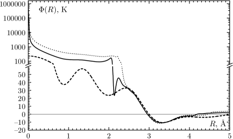
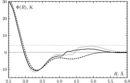
a)                                                                                        b)

Figure 1: The potential $\Phi(R)$ with short-range interactions in hard sphere approximation (HS-$\rho^{2}$ — solid line, PY — dotted line) compared with results of our previous work [2] (dashed line).

3.2 Softened repulsion

The true repulsive part of the potential should be a bit “softened”. It is easier to formulate this “softening” in the terms of Meyer function $f(R)$:

$$f(R)=e^{-\beta\Phi(R)}-1$$ (8)

that stays finite while $\Phi(R)$ can have infinities, see (7).

For the hard sphere system $f(R)$ reads

$$f^{\rm HS}(R)=\theta(R-a)-1=\left\{\begin{array}[]{cl}-1,&R\leq a\\ 0,&R>a\end{array}\right.,$$ (11)

In this terms, the softening means that the straight step of the Meyer function of hard sphere must be slightly “rounded”. Here we consider the variants of this “rounding”.

Let us suppose the power dependence in $\Phi^{0}(R)$: $\Phi^{0}(R)\propto 1/R^{n}$. Then the kinetic energy operator in the Schrödinger equation gives:

$$-{\hbar^{2}\over 2m}{\partial^{2}\over\partial R^{2}}\,e^{-(A/R)^{n}}=-{\hbar^{2}\over 2m}{n^{2}\over R^{2}}\left({A\over R}\right)^{2n}e^{-(A/R)^{n}}+O(1/R^{n+2}).$$ (12)

Thus, the power $2n+2$ must equal the power of inverse distance in the repulsive part of real potential. Assuming it to be the Lennard–Jones potential we obtain $n=5$.

Another way is to round the corners in the Meyer function via direct accepting its form. For instance, like in the previous case:

$$f(R)=e^{-(A/R)^{n}}-1.$$ (13)

The value of $n$ should be taken large (larger than 5) in order to resemble the hard sphere step.

The first case (Lennard–Jones repulsion, $n=5$) will be called “soft spheres” (SS), and the second one (directly accepted repulsion) will be denoted as “almost hard spheres” (AHS).

Let us choose the following values for AHS quantities in (13):

$$A=2.1\ {\rm\AA},\qquad n=12.$$ (14)

The Meyer function then becomes quite close to the hard sphere step, see Fig. 2. That is the reason why we call it “almost hard spheres”.

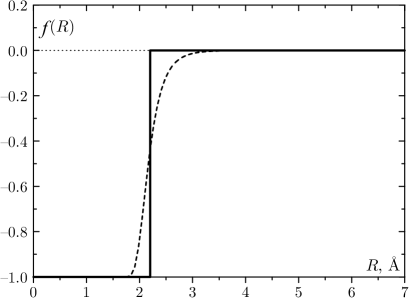
Figure 2: Meyer functions of hard spheres (solid line) and almost hard spheres (dashed line).

We have calculated the structure factor of the softened repulsive part using the PY approximation. Since we do not need big accuracy, only the first iteration in the Ornstein–Zernike equation was used. Our results show that the potential curve does not differ much from that of our previous work [2], see Fig. 3.

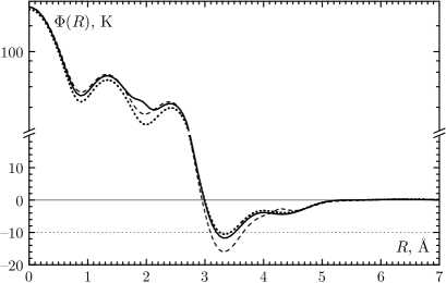
Figure 3: The potential $\Phi(R)$ with short-range interactions in SS (dashed line) and AHS (solid line) approximation compared with results of our previous work [2] (dotted line)

In spite of large difference in $1/R$ powers (5 and 12), the results do not yield to much different behaviour in the region of small $R$: it still resembles that of [2]. From this point of view, the reason must be in principal difference between soft and hard spheres, namely in the analyticity or non-analyticity of Meyer function that leads to different types of damping at large $q$ for the structure factor and, as a result, for the Fourier image $\nu_{q}$.

Another fact concerns the region of potential well. One can see that the increasing of $1/R$ power from 5 to 12 moves the depth of the well closer to that of obtained from the hard sphere approximation. On the other hand, similar value was obtained in [2] and it appears not to differ much from the results of computer simulations [7, 8] and the computations with adjustable parameters [3, 4, 5, 6]. Those results might be found in Table 1.

Potential	$\Phi(0)$, K	Well	Extra Hill
Ref. References	$\simeq 240$	$-10.59$ K at 3.34 Å	$0.26$ K at 6.41 Å
HS – $\rho^{2}$	$\infty$	$-10.86$ K at 3.32 Å	$1.99$ K at 4.84 Å
HS – PY	$\infty$	$-11.55$ K at 3.27 Å	$3.64$ K at 4.94 Å
AHS	$\simeq 240$	$-11.76$ K at 3.34 Å	$0.23$ K at 6.31 Å
SS	$\simeq 230$	$-15.95$ K at 3.32 Å	$0.27$ K at 6.44 Å
Glued	$\infty$	$-11.72$ K at 3.33 Å	$0.23$ K at 6.31 Å
Ref. References	—	$-11.01$ K at 3.00 Å	no hill
Ref. References	$2\cdot 10^{6}$	$-11.04$ K at 2.99 Å	no hill

Table 1. Parameters of the potential curve for different types of potential.

The extra-hill was obtained on our potential curves at the interatomic distances of $\simeq 5-7$ Å. We consider it as a consequence of solving the problem of interaction between helium atoms via quantum equations. But the large values of hill maxima obtained in the case of hard-sphere interaction should be treated as the result of Meyer function non-analyticity. We claim it since the correspondent values in the case of soft spheres and almost hard spheres are commensurable with the value from [2].

The region of small $R$ values is probably the most complicated one. It seems that one should accept the hard-sphere approximation in order to obtain a good description here. We tried to join the advantages of the PY short-range part with those of the AHS long-range part by just “gluing” this two data sets at the point of 3.25 Å. The left side corresponds to PY; the right side – to AHS.

One can notice that there is a constant positive difference between the minimum position (the equilibrium interatomic distance) of the potentials discussed in this work and of those calculated by Aziz et al. We consider it as a consequence of the effective nature of our potentials. Let us consider the model of hard spheres with diameter $a$ in order to illustrate this statement. The equilibrium distance between two atoms in the system of two atoms is obviously $a$. But if one considers the system of three particles than the average distance slightly increases, namely by 5 per cent. Thus, the difference in approximately 10 per cent in our case might be at least partially considered as a consequence of such a geometric effect.

4 Energy and sound velocity

One can calculate the potential energy $\Phi$ of the system at 0 K using the relation [15]:

$$\Phi=N{\rho\nu_{0}\over 2}+\sum_{\bf q\neq 0}{\rho\nu_{q}\over 2}\left({1\over\alpha_{q}}-1\right),$$ (15)

$$\alpha_{q}=\sqrt{1+{2\rho\nu_{q}\over\varepsilon_{q}}},\qquad\varepsilon_{q}={\hbar^{2}q^{2}\over 2m}.$$ (16)

The total energy $E$ reads:

$$E=\Phi+\sum_{\bf q\neq 0}{\varepsilon_{q}\over 4}\,{(\alpha_{q}-1)^{2}\over\alpha_{q}}.$$ (17)

The quantity $\rho\nu_{0}$ in these equation must be substituted with $mc^{2}$ where $c$ is the sound velocity in ⁴He. The value $mc^{2}=\rho\nu_{0}$ corresponds to the RPA and we want to have the next, postRPA approximation. Thus, the corrected expression reads [13]:

$$mc^{2}=\rho\nu_{0}-{1\over 8N}\sum_{\bf q\neq 0}\varepsilon_{q}{(\alpha_{q}-1)^{2}\over\alpha_{q}}.$$ (18)

We give the results discussed above in the Table 1 for the comparison. The left hand values of sound velocity correspond to the RPA ($mc^{2}=\rho\nu_{0}$), while the right-hand values reflect the correction [13].

Potential	$\Phi/N$, K	$E/N$, K	$c$, m/s
Ref. References	$-15.5$	$-7.8\$	292 vs 238
HS-$\rho^{2}$ ${}^{\rm a})$	$+18.1$	$+38.8\$	407 vs 524
AHS	$-21.6$	$-12.0\$	297 vs 240
SS	$-29.1$	$-18.6\$	254 vs 182
Glued	$-16.7$	$-8.0\$	324 vs 262
Ref. References$\,{}^{\rm b})$	$-21.7$	$-7.1\$	241
Experiment		$-7.17\,^{\rm c})$	240.3$\,{}^{\rm d})$

^a)We do not give data for the potential obtained using $S^{\rm PY}$ since in this case one cannot obtain a “good” $\alpha_{q}$: value of $1+2\rho\nu_{q}/\varepsilon_{q}$ is negative for some values of $q$.
${}^{\rm b})$Calculation using potential [3].
${}^{\rm c})$Ref. References.
${}^{\rm d})$This value corresponds to the sound velocity at saturated vapour pressure for $T=0.1$ K [16]. Ref. References gives 237.8 m/s at $T=0.8$ K. These values are not strictly experimental but it is possible to consider them as the averaged experimental ones since they are calculated using the well-analyzed equation of state.

Table 2. Energy and sound velocity with different potentials.

As might be seen from the Table 2, the HS model for the short-range repulsion yields to incorrect values for energy and the sound velocity. Unfortunately, we did not find the universal potential satisfying the requirements to describe the total energy and the potential energy with similar accuracy. The best fit for both these quantities is found in the case of “glued” potential but the method of its obtaining looks very artificially. One can see that the best fit of the potential energy is found in the AHS approximation for the short-range repulsion. On the other hand, previously obtained potential [2] remains the best of those considered here due to the values of the total energy and the sound velocity.

Therefore, three potential will be used in our further works: the potential obtained in [2], the potential with AHS short-range repulsion, and the “glued” potential. The comprehensive analysis of thermodynamic and transport properties that might be calculated and compared with the experiment or the computer simulations will judge the most suitable model potential.

References

- [1] [∗]e-mail: andrij@ktf.franko.lviv.ua .
- [2] I. O. Vakarchuk, V. V. Babin, A. A. Rovenchak, J. Phys. Stud. 4, 16 (2000).
- [3] R. A. Aziz, V. P. S. Nain, J. S. Carley, W. L. Taylor, G. T. McConville, J. Chem. Phys. 70, 4430 (1979).
- [4] R. A. Aziz, M. J. Slaman, J. Chem. Phys. 94, 8047 (1991).
- [5] R. A. Aziz, M. J. Slaman, A. Koide, A. R. Allnatt, W. J. Meath, Mol. Phys. 77, 321 (1992).
- [6] A. R. Janzen and R. A. Aziz, J. Chem. Phys. 107, 914 (1997).
- [7] J. A. Anderson, C. A. Traynor, B. M. Boghosian, J. Chem. Phys. 99, 345 (1993).
- [8] K. T. Tang, J. P. Toennies, C. L. Yiu, Phys. Rev. B 74, 1546 (1995).
- [9] J. Boronat, J. Casulleras, Phys. Rev. B 49, 8920 (1994).
- [10] Svensson E. C., Sears V. F., Woods A. D. B., Martel P. Phys. Rev. B, 21, 8 (1980). ???
- [11] R. De Bruyn Ouboter, C.N. Yang, Physica B 44, 127 (1987).
- [12] I. A. Vakarchuk, Teor. Mat. Fiz. 80, 439 (1989); 82, 438 (1990).
- [13] I. A. Vakarchuk, I. R. Yukhnovsky, Teor. Mat. Fiz. 40, 100 (1979).
- [14] R. Balescu, Equilibrium and nonequilibrium statistical mechanics (New York: Wiley, 1975).
- [15] I. O. Vakarchuk, J. Phys. Stud. 1, 25 (1996).
- [16] R. D. McCarthy, Nat. Bur. Stand. (U.S.), Tech. Note 1029, (1980).
- [17] V. D. Arp, R. D. McCarty, D. G. Friend, Natl. Inst. Stand. Technol. Tech. Note 1334 (revised) (1998).