How to escape Aharonov-Bohm cages ?

Abstract

We study the effect of disorder and interactions on a recently proposed magnetic field induced localization mechanism. We show that both partially destroy the extreme confinement of the excitations occuring in the pure case and give rise to unusual behavior. We also point out the role of the edge states that allows for a propagation of the electrons in these systems.

I Introduction

The dynamics of a quantum particle in a periodic potential in the presence of a uniform static magnetic field has revealed many beautiful effects and has been the subject of ongoing researches for several decades. The competition between the two characteristic length scales involved, namely the lattice period and the magnetic length produces a very complex pattern of energy levels. In two dimensions, this leads to fractal structures in the spectrum anticipated by Azbel[1], and further studied by Hofstadter[2], Claro and Wannier[3], Rammal[4], and many others. Some striking experimental manifestations of these effects have been found in macroscopic properties of two-dimensional superconducting wire networks, such as the variation of the critical temperature with respect to the external magnetic field, the magnetization or the critical current. The connection between the linearized Ginzburg-Landau equations used to describe these wire networks close to the superconducting transition, and the tight-binding spectrum of electrons had been established slightly before these experiments by De Gennes[5] and Alexander[6].

More recently, a surprising effect has been presented in ref. [7] in a two-dimensional lattice with hexagonal symmetry, the so-called ${\cal T}_{3}$ lattice displayed in Fig. 1. For some values of the magnetic field corresponding to half a flux quantum per elementary tile, the energy spectrum of a tight-binding model with nearest neighbor hopping collapses into three highly degenerate levels. Furthermore, we have shown that it is possible to build energy eigenstates where the probability to find an electron is non vanishing only in a finite size cluster which we have called an Aharonov-Bohm cage. This corresponds to a localization mechanism due to quantum interferences of Aharonov-Bohm type between paths enclosing a half-integer number of flux quanta. For instance, if an electron is initially located on a given site of the lattice, it will never propagate beyond the boundary of the cage associated to this site, provided the magnetic field is chosen properly, as discussed above.

Since this theoretical observation, several experiments have searched for manifestations of these cages on real systems. A serie of investigations on superconducting wire networks has been completed by Abilio et al.[8] and by Serret et al.[9] providing a good agreement between predictions and measurements of the critical temperature and the critical current. In addition, the unusual nature of the mixed state for half a flux quantum per elementary tile has been clearly indicated by a strong reduction of the critical current, and by magnetic decoration experiments which shows a very highly disordered vortex pattern[9, 10].

A slightly more direct probe of this localization effect has been provided by transport measurements in mesoscopic lattices carved in a two-dimensional electron gas at the interface of GaAs/GaAlAs heterostructures[11]. In theses systems, the number of tranverse conduction channels in the wires can be very small (a few units), and the mean free path much larger than the distance between two nearest neighbor nodes. At intermediate magnetic fields, Naud et al. have clearly observed a periodic modulation of the magnetoconductance with a period of one flux quantum per plaquette ($h/e$). In the same experimental conditions, a square lattice does not show these oscillations. It seems more than plausible that these $h/e$-periodic oscillations seen on ${\cal T}_{3}$ lattice could be attributed to the Aharonov-Bohm cages. Indeed, this localization mechanism establishes a strong difference in the tranport properties between integer and half integer fluxes, which is expected to survive in the presence of a weak enough disorder as discussed in ref. [12].

These experiments clearly motivate us to address the question of the robustness of these cages in the presence of “real life” perturbations such as disorder, finite size effects and electron-electron interactions. The main purpose of this paper is to attempt to bridge the gap between the very idealized tight-binding model initially studied in ref. [7], and the experimental systems mentioned above. As a general trend, we will show that if the cages are in themselves very fragile, their existence in the ideal system induces a few remarkable features for the perturbed ones. The underlying reason for this is that these perturbations act on a very degenerate system, and as often in physics, degenerate perturbations are expected to induce some very interesting phenomena. One of the most famous example is, of course, the fractional quantum Hall effect where the degeneracy of the kinetic energy at fractional filling factors opens the way to the formation of strongly correlated many-body exotic states such as the Laughlin liquid[13].

This paper is organized as follows. Section II presents a detailed discussion of the butterfly-like energy spectrum for a tight-binding model on the ${\cal T}_{3}$ lattice. Section III focusses on half integer fluxes for which the cages appears. Several viewpoints are given to provide a simple physical intuition of what happens in the system. This enables us to show other examples of lattices for which Aharonov-Bohm cages exist. Section IV discusses disorder effects still within the tight-binding framework. So, it is complementary to the previous study presented in ref. [12] where the continuous wire model was analyzed, in connection to the experiments on two-dimensional gases. Here, we investigate some properties of one particle eigenstates such as the inverse participation ratio as a function of the disorder strength and the magnetic field. Section V is devoted to edge states. These states are found to be confined in a finite width strip along the boundaries of the sample. We outline the subtleties involved in the translation from the tight-binding model properties to those of the continuous one-dimensional wire networks. Finally, section VI adresses interactions effects in the context of the Hubbard model. Most of the results deal with the two electron case. In agreement with a previous study for the chain of loops[14], we find that interactions are able to create some extended and dispersive two particle eigenstates. This can be viewed as a kind of interaction induced delocalization phenomenon, similar to the one discussed by Shepelyansky for disordered systems[15]. The presence of the cages in the non interacting case is reflected by the fact that these extended states involve a close binding of the two particles in real space, even if the local interaction is repulsive. We also give some ground state configurations for a finite density of particles and we show that the energy per particle has a singular behaviour when the number of electrons per site becomes larger than 1/3. In the last section, we conclude and discuss the experimental relevance of our work. Technical details for the two interacting particles problem can be found in the appendix A.

II Spectral properties

We consider the ${\cal T}_{3}$ lattice displayed in Fig. 1 which is a bipartite periodic structure with 3 sites per unit cell: one 6-fold coordinated site $A$ and two 3-fold coordinated site $B$ and $C$.

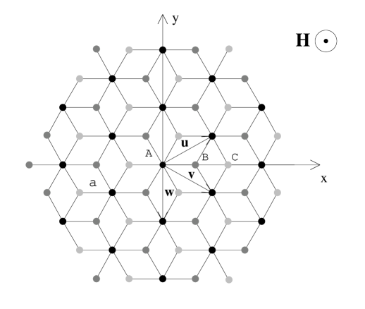
FIG. 1.: A piece of the ${\cal T}_{3}$ lattice embedded in the perpendicular magnetic field ${\bf H}$ ; $a$ denotes the lattice spacing.

This tiling can also be seen as the dual of the most famous Kagomé lattice[16]. We consider a tight-binding hamiltonian defined by :

$$H_{0}=\sum_{<i,j>}t_{ij}|i\rangle\langle j|$$ (1)

where $|i\rangle$ is a localized orbital on site $i$. When ${\bf H}=0$, the hopping term $t_{ij}=1$ if $i$ and $j$ are nearest neighbors and $0$ otherwise. In the presence of a magnetic field[17], $t_{ij}$ is multiplied by a phase factor $e^{i\gamma_{ij}}$ involving the vector potential ${\bf{A}}$ :

$$\gamma_{ij}={\frac{2\pi}{\phi_{0}}}\int_{i}^{j}{\bf A}.\mbox{d}{\bf l}\mbox{,}$$ (2)

where $\phi_{0}=hc/e$ is the flux quantum. In the following, we focus on the case of a uniform magnetic field ${\bf H}=H{\bf z}$ which can be obtained, for example, with the Landau gauge ${\bf A}=H(0,x,0)$, and we denote by $\phi=Ba^{2}\sqrt{3}/2$ the magnetic flux through an elementary rhombus.

Let us first briefly analyze the zero field case ${\bf H}=0$. In this case, the one-particle spectrum is given by the following dispersion relation :

$$E_{\pm}\left({\bf k}\right)=\pm\sqrt{6+4\left[\cos({\bf k}.{\bf u})+\cos({\bf k}.{\bf v})+\cos({\bf k}.{\bf w})\right]}\mbox{,}$$ (3)

where ${\bf u}=a(3/2,\sqrt{3}/2)$ and ${\bf v}=a(3/2,-\sqrt{3}/2)$ are the vectors of the primitive cell (see Fig. 1), ${\bf w}={\bf v-u}$, and where ${\bf k}$ is a wave vector lying in the first Brillouin zone. The associated eigenstates are standard Bloch waves. In addition, there is a non dispersive band at $\varepsilon_{0}=0$ resulting from the bipartite character of the structure, and whose degeneracy is given by the difference between the number of 3-fold and 6-fold coordinated sites. Since its origin is purely topological, this energy will always be an eigenvalue for any ${\bf H}$, with the same degeneracy. The density of states, originally computed by Sutherland[18], is shown in Fig. 2.

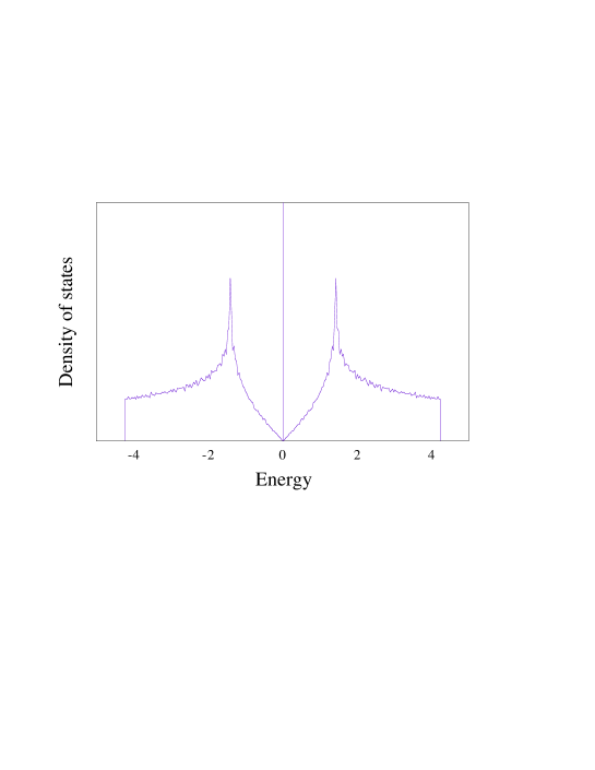
FIG. 2.: Density of states of the ${\cal T}_{3}$ lattice for ${\bf H}=0$.

For ${\bf H}\neq 0$, the spectrum is of course much more complex since there remains only one translational invariance along the $y$ direction due to the gauge choice, so that the eigenfunctions can be written as :

$$\varphi_{j}(x,y)=\psi_{j}(x)e^{ik_{y}y},\hskip 4.30554ptk_{y}\in\left[0,2\pi/{a\sqrt{3}}\right]\mbox{.}$$ (4)

where the index $j=A,B,C$. Thus, the secular equations read :

$$\varepsilon\psi_{A}(x) = \psi_{B}(x+a)+\psi_{B}\left(x-{a\over 2}\right)2\cos\left[{\gamma\over a}\left(x-{a\over 4}\right)+\kappa\right]+$$ (6)

$$\psi_{C}(x-a)+\psi_{C}\left(x+{a\over 2}\right)2\cos\left[{\gamma\over a}\left(x+{a\over 4}\right)+\kappa\right]$$

$$\varepsilon\psi_{B}(x) = \psi_{A}(x-a)+\psi_{A}\left(x+{a\over 2}\right)2\cos\left[{\gamma\over a}\left(x+{a\over 4}\right)+\kappa\right]$$ (8)

$$\varepsilon\psi_{C}(x) = \psi_{A}(x+a)+\psi_{A}\left(x-{a\over 2}\right)2\cos\left[{\gamma\over a}\left(x-{a\over 4}\right)+\kappa\right]\mbox{ , }$$ (10)

where $\kappa=k_{y}a\sqrt{3}/2$, and $\gamma=2\pi\phi/\phi_{0}=2\pi f$. Note that with the origin $O$ chosen in Fig. 1, $x$ only takes integer or half-integer values. If one looks for solutions $\varepsilon\neq 0$ of the secular system, one can substitute (8) and (10) in (6) to obtain an effective one-dimensional equation that only involves six-fold coordinated sites :

$$(\varepsilon^{2}-6)\psi_{m} = 2\cos\left({\frac{\gamma}{2}}\right)\left\{2\cos\left[{\frac{3\gamma}{2}}\left(m+{\frac{1}{2}}\right)+\kappa\right]\psi_{m+1}\right.+\left.2\cos\left[{\frac{3\gamma}{2}}\left(m-{\frac{1}{2}}\right)+\kappa\right]\psi_{m-1}\right.+2\cos\left(3\gamma m+2\kappa\right)\psi_{m}\bigg{\}}\mbox{ , }$$ (11)

where $\psi_{m}=\psi_{A}({x=3ma/2})$, $(m\in{\bf Z})$. As it can be readily seen in Fig. 1, the six-fold coordinated sites form a triangular lattice so that Eq. (11) has to be compared to those derived by Claro and Wannier for the triangular lattice[3] :

$$\varepsilon_{T}\psi_{m} = 2\cos\left[\gamma_{T}\left(m+{\frac{1}{2}}\right)+\kappa\right]\psi_{m+1}+2\cos\left[\gamma_{T}\left(m-{\frac{1}{2}}\right)+\kappa\right]\psi_{m-1}+2\cos(2\gamma_{T}m+2\kappa)\psi_{m}$$ (12)

with similar notations. So, the ${\cal T}_{3}$ lattice spectrum can be simply obtained from the triangular lattice spectrum by setting $\gamma_{T}=3\gamma/2$, since one has :

$$\varepsilon^{2}-6=2\cos\left({\frac{\gamma}{2}}\right)\varepsilon_{T}\mbox{.}$$ (13)

Since the tiling is bipartite, the spectrum is symmetric ($\varepsilon\leftrightarrow-\varepsilon$). Moreover, Eq. (11) displays a translation symmetry $f\rightarrow f+n\>(\forall n\in{\bf Z})$ and a reflection invariance about half-integer values of $f$. We thus limit our analysis to $0\leq f\leq 1/2$. For rational values of $f=p/q$ ($p,q$ mutually prime), the system (11) becomes closed after a translation by $q$ periods and the spectrum is made up of $2q$ bands. Note that, when $q=3q^{\prime}$ $(q^{\prime}\in{\bf N})$, this period is actually reduced by a factor $3$ and the spectrum has only $2q^{\prime}$ bands. In particular, for $f=1/3$, one can exactly compute the dispersion relation :

$$\varepsilon^{2}(\kappa,k_{x})-6=-2\cos(2\kappa)+4\cos(\kappa)\cos(k_{x}a)\mbox{ , }$$ (14)

where $(k_{x},\kappa)\in[0,2\pi/a\sqrt{3}]\times[0,\pi]$. For this flux, the spectrum spreads from $-3$ to $+3$ and is gapless. Figure 3 shows the ${\cal T}_{3}$ lattice spectrum support versus the reduced flux $f$. The most spectacular and unusual feature is that, for $f=1/2$, the spectrum collapses into three eigenvalues $\varepsilon_{0}=0$ and $\varepsilon_{\pm}=\pm\sqrt{6}$ as it can be readily seen from Eq. (13).

FIG. 3.: Spectrum of the ${\cal T}_{3}$ lattice as a function of the reduced flux.

This is all the more curious that usually, for an infinite periodic structure and for rational values of $f$, the spectrum is absolutely continuous (band-like). Here, it behaves as a super-atom with three infinitely degenerate levels with equal spectral weights $1/3$. The existence of these non dispersive bands suggests the possibility to build Wannier-type localized eigenstates. This remarkable fact is, for any electron density, susceptible to induce original physical properties reminiscent of those of a localized system.

III The Aharonov-Bohm cages

In this section, we shall analyze these properties from the quantum dynamics point of view by characterizing the spreading of a wave packet in the ${\cal T}_{3}$ lattice, at $f=1/2$. To achieve this, it is worth focusing on the spectral charateristics at a local level. The magnetic field being uniform, the whole spectrum is indeed recovered from the local density of states (LDOS) on the two different types of sites. At this point, it is more convenient to shift from the above Landau gauge to a cylindrical (symmetric) gauge defined by ${\bf A}=H(-y/2,x/2,0)$ that respects the discrete rotational symmetry existing locally. We proceed to an analytic Lanczos tridiagonalization using the recursion method[19]. The principle of this algorithm is to generate an semi-infinite chain according to the recursive relation :

$$b_{n+1}|\varphi_{n+1}\rangle=(H_{0}-a_{n})|\varphi_{n}\rangle-b_{n}|\varphi_{n-1}\rangle$$ (15)

which allows to evaluate the LDOS on the initial orbital $|\varphi_{0}\rangle$. The diagonal and off-diagonal terms ($a_{n}$,$b_{n}$) are obtained by requiring the normalization of the orbitals $|\varphi_{n}\rangle$. Note that in our case, all the diagonal elements $a_{n}$ vanish because : (i) the structure is bipartite, (ii) $H_{0}$ is purely off-diagonal.

Let us first compute the recursion chain associated to a six-fold coordinated site and choose, as initial orbital, $|\varphi_{0}\rangle=|0\rangle$ (see Fig .4). One has :

$$H_{0}|\varphi_{0}\rangle=\sum_{i=1}^{6}|i\rangle\hskip 12.91663pt\Rightarrow\hskip 12.91663ptb_{1}=\sqrt{6}\,,\>|\varphi_{1}\rangle={1\over\sqrt{6}}\sum_{i=1}^{6}|i\rangle\mbox{ . }$$ (16)

The first recursion orbital $|\varphi_{1}\rangle$ is a linear symmetric combination of the first shell sites (three-fold coordinated grey sites). At the next step, one obtains :

$$H_{0}|\varphi_{1}\rangle=b_{1}|\varphi_{0}\rangle+2\cos(\pi f){1\over\sqrt{6}}\sum_{i=7}^{12}|i\rangle\hskip 12.91663pt\Rightarrow\hskip 12.91663ptb_{2}=2\cos(\pi f)\,,\>|\varphi_{2}\rangle={1\over\sqrt{6}}\sum_{i=7}^{12}|i\rangle\mbox{ . }$$ (17)

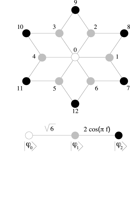
FIG. 4.: Aharonov-Bohm cage associated to the six-fold coordinated sites and its recursion chain. For $f=1/2$, the black sites are never visited by a wave packet initially localized on the central site (white).

For $f=1/2$, $b_{2}=0$ so that the LDOS is reduced to two values $\varepsilon_{\pm}=\pm\sqrt{6}$ with an equal spectral weight $1/2$. This effect can be simply understood in terms of Aharonov-Bohm effect. Indeed, the amplitude of probability ${\cal A}_{0\rightarrow 2\rightarrow 9}$ to go for example, “in two steps”, from 0 to 9 via 2, is exactly the opposite of ${\cal A}_{0\rightarrow 3\rightarrow 9}$, so that the resulting amplitude is zero. Then, any wave packet initially localized on a six-fold coordinated site ($|\psi(t=0)\rangle=|0\rangle$) is completely trapped inside what we have called an Aharonov-Bohm cage[7] whose precise definition is given below. One can easily determine its time evolution that is periodic and given by :

$$|\psi(t)\rangle=\cos\left(\sqrt{6}t\right)|\varphi_{0}\rangle-i\sin\left(\sqrt{6}t\right)|\varphi_{1}\rangle\mbox{ . }$$ (18)

In particular, the autocorrelation function $|\langle 0|\psi(t)\rangle|^{2}=\cos^{2}\left(\sqrt{6}t\right)$ for $f=1/2$, whereas for $f=0$ :

$$|\langle 0|\psi(t)\rangle|^{2}=\left({3\sqrt{3}\over 8\pi^{2}a^{2}}\int\int_{1BZ}\cos\left(E\left({\bf k}\right)t\right){\mbox{d}}{\bf k}\right)^{2}$$ (19)

($1BZ$ stands for first Brillouin zone) and behaves at large $t$ as :

$$|\langle 0|\psi(t)\rangle|^{2}\simeq{3\over 8\pi^{2}t^{2}}\left[\sin\left(3\sqrt{2}t\right)+\sqrt{3}\cos\left(\sqrt{2}t\right)\right]^{2}\mbox{ . }$$ (20)

We emphasize that for a generic rational $f\neq 1/2$, the hamiltonian is periodic and one expects $|\langle 0|\psi(t)\rangle|^{2}\sim 1/t^{2}$. A contrario, when $f$ is irrationnal, the hamiltonian is quasiperiodic and one expects, as for the square lattice [20], $|\langle 0|\psi(t)\rangle|^{2}\sim 1/t^{2\alpha}$ with $\alpha<1$ since the spectrum should be singular continuous.

The same type of recursion calculation can be made for the three-fold coordinated sites. In this case, one easily obtains :

$$b_{1} = \sqrt{3}\,,$$ (21)

$$b_{2} = \sqrt{4\cos^{2}(\pi f)+3}\,,$$ (22)

$$b_{3} = \sqrt{8\cos^{2}(\pi f)+4\left[\cos(\pi f)+\cos(3\pi f)\right]^{2}\over 4\cos^{2}(\pi f)+3}\mbox{ , }$$ (23)

so that $b_{3}=0$ for $f=1/2$, and the LDOS on this type of site reduces to the $\varepsilon_{0}=0$ (spectral weight 1/2), and $\varepsilon_{\pm}=\pm\sqrt{6}$ (spectral weight 1/4). The quantum evolution of a wave packet initially localized on such a site is therefore, as previously, confined in a cage displayed in Fig. 5 that is larger than the one obtained for the 6-fold coordinated sites.

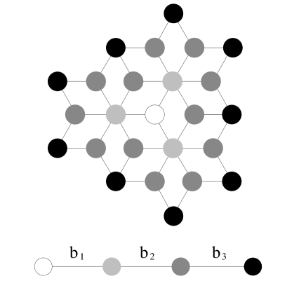
FIG. 5.: Aharonov-Bohm cage associated to the three-fold coordinated sites and its recursion chain.

Finally, since the ${\cal T}_{3}$ lattice is only made up of 6-fold and 3-fold coordinated sites, any wave packet (with a finite initial extension) will be confined inside a bound Aharonov-Bohm cage at $f=1/2$. We emphasize that this localization phenomenon must be understood from the quantum dynamics point of view. Indeed, contrary to the Anderson localization, the eigenstates of the system are not exponentially localized, and not even localized at all since the high degeneracy allows one to build any type of eigenstates (possibly extended).

To proceed further, it is necessary to give a precise definition of these Aharonov-Bohm cages. For a given wave packet $|\psi\rangle$ submitted to a magnetic field characterized by a reduced flux $f$, we define the Aharonov-Bohm cage ${\cal C}^{f}_{\psi}$ as the set of sites visited by this initial wave packet during its evolution. In general, ${\cal C}^{f}_{\psi}$ is infinite, but as shown previously, it can, for specific values of the magnetic field ($f=1/2$ for the ${\cal T}_{3}$ lattice), be bound. To analyze the cage structures for any independent electron model, it is sufficient to characterize the cages of all inequivalent sites. Indeed, the superposition principle implies that if $|\psi(t=0)\rangle=\sum_{i=1}^{n}\alpha_{i}\,|i\rangle$, one has the following property :

$${\cal C}_{\psi}^{f}\>{\subset}\>\bigcup_{i=1}^{n}\>{\cal C}_{i}^{f}\mbox{ . }$$ (24)

With this definition, several cases can be encountered :

• all cages are unbound for any $f$ (ex : square lattice, triangular lattice, honeycomb) ;

• some cages are bound for particular values of $f$ (ex : the Penrose tiling and the octagonal tiling displayed in Fig. 6) ;

• all the cages are bound for the same values of $f$ (ex : ${\cal T}_{3}$ lattice).

FIG. 6.: Two examples of structure presenting bound cages for special initial conditions of the wave packet localized at the center of some 5-fold symmetric stars for the Penrose tiling (left) and 8-fold symmetric stars for the octogonal tiling (right).

This latter case, that we will call fully confined structure, can be met for other tilings. As an example, we have displayed in Fig. 7 , the so-called ${\cal T}_{4}$ lattice which can be obtained by deforming an approximant with $14$ sites per unit cell of the octagonal tiling.

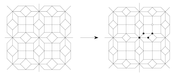
FIG. 7.: A piece of the periodic ${\cal T}_{4}$ tiling before (left) and after deformation (right). The five different types of sites are represented ($\bullet,\circ$).

This structure has exactly the same physical properties as the ${\cal T}_{3}$ lattice at $f=1/2$ ($f$ refers here to the reduced flux measured in the smallest tile). Thereafter, we shall consider a light version of this tiling obtained by eliminating the sites $\circ$ and their related bonds (see Fig. 7). The resulting structure is simply a set of connected 8-fold symmetric stars with two different lengths whose ratio is equal to $\sqrt{2}$. We thus allow for two different hopping terms $t_{L}$ and $t_{S}$ for long and short edges respectively. For $f=1/2$, it is always possible to choose a gauge such that all the $t_{ij}$’s are real. A possible choice is represented in Fig. 8.

FIG. 8.: A possible gauge choice for the ${\cal T}_{4}$ lattice at $f=1/2$. All the Peierls terms are equal to $+1$ except those represented by dotted lines that are equal to $-1$. For clarity we have omit the hopping term $t_{L,S}$.

Note that this gauge has the same periodicity as the structure. This is quite surprising since it is not the generic case (see next section for the ${\cal T}_{3}$ lattice). It is then easy to diagonalize $H_{0}$ and to obtain the thirteen following eigenvalues : 0 (three-fold degenerate), $\pm\sqrt{2t_{L}^{2}+2t_{S}^{2}}$ (two-fold degenerate), $\pm\sqrt{t_{S}},\pm\sqrt{4t_{L}^{2}+4t_{S}^{2}},$ and $\pm\sqrt{4t_{L}^{2}+2t_{S}^{2}}$. For any hopping terms $t_{L,S}$ these eigenvalues do not depend on any wave vector and thus form the exact analogous of the non dispersive bands obtained in the ${\cal T}_{3}$ lattice.

We would like to point out that fully confined systems can also be obtained in one dimension. We have shown in Fig. 9 a quasi-one-dimensional structure that clearly displays bound Aharonov-Bohm cages at $f=1/2$. Its eigenspectrum is, as for the ${\cal T}_{3}$ lattice, made up of three non dispersive bands with energies $0,\pm 2$.

FIG. 9.: The simplest example of a periodic fully confined structure for $f=1/2$.

After this detailed description of this magnetic field induced localization, it is natural to wonder if this phenomenon is robust to various type of “perturbations”. For example, a non uniform magnetic field has been shown to drastically change the energy spectrum and the localization properties of the system providing a complete destruction of the cages[21]. In the next section, we study the effect of different kind of disorder and we show that, the destructive interference that leads to the Aharonov-Bohm cages are partially destroyed.

IV The disorder

A first natural way to introduce disorder in a system is to directly modify its structure by incorporating defects. In the case of the ${\cal T}_{3}$ lattice, such defects can be simply generated by a local elementary flip of three tiles as shown in Fig. 10.

FIG. 10.: Elementary flip for two-dimensional tilings.

For $f=1/2$, it is clear that a finite number of flips does not modify the bound nature of the cages since, sooner or later, a given wave packet will be embedded in the “pure” ${\cal T}_{3}$ lattice geometry which is responsible of the confinement. Nevertheless, one can wonder if this feature still holds for a finite density of such defects. Indeed, if we consider a large number of flips in order to get closer and closer to a random tiling configuration[22], we expect the destructive Aharonov-Bohm interferences to completely disappear. It would be, in this case, interesting to determine the critical density below which all the cages remains bound. This could be achieved by considering an extended initial state and by computing its time evolution for different realizations of the disorder and for different flip densities. Note that this value should be easily understood in terms of cages percolation threshold.

Another possible way to introduce disorder is to randomly modulate either off-diagonal or diagonal terms in the hamiltonian. In this study, we mainly focus on the latter case and consider the following hamiltonian :

$$H_{dis.}=\sum_{\langle i,j\rangle}t_{ij}\,|i\rangle\langle j|+\sum_{i}V_{i}\,|i\rangle\langle i|\mbox{ , }$$ (25)

where the $t_{ij}$ are defined as in (1), and where the on-site energies $V_{i}$ are mutually independent gaussian random variable with variance $\sigma^{2}$.

As the strength of disorder increases, the strongly localized cage eigenstates begin to spread over larger distances. In some sense, a weak disorder increases the one-particle localization typical length ! However, since the system is two-dimensional, we expect the overall localization length to be finite for any value of $\sigma\neq 0$ and for any energy. For a given reduced flux $f$, as $\sigma$ is increased from zero, the one-particle eigenstates first get mixed within the energy bands of the pure model. This regime corresponds to the standard Anderson localization. This lasts until $\sigma$ becomes of the order of some energy gaps allowing then for interband mixing.

For $f=1/2$, the remarkable structure of the spectrum at zero disorder is responsible for the absence of the first disorder induced localization regime. Therefore, we expect, in this case, that most observables will depend only weakly on $\sigma$, as long as $\sigma$ remains smaller than the gaps. To analyze this problem, it is interesting to construct an effective model in the lowest energy subspace of $H_{0}$, expressed in the localized cage basis (see Fig. 19 in the next section). Denoting the normalized cage eigenstates associated to $\varepsilon_{-}=-\sqrt{6}$ centered around the six-fold coordinated sites ${\bf r}$ by $|{\bf r}\rangle$, this effective hamiltonian has the form :

$$H_{eff.}=\sum_{\langle{\bf r},{\bf r}^{\prime}\rangle}\tilde{t}_{{\bf r},{\bf r}^{\prime}}\,|{\bf r}\rangle\langle{\bf r}^{\prime}|+\sum_{\bf r}\tilde{V}_{\bf r}\,|{\bf r}\rangle\langle{\bf r}|\mbox{ , }$$ (26)

where $\langle{\bf r},{\bf r}^{\prime}\rangle$ stands for the sum over nearest neighbors in the triangular lattice generated by the the six-fold coordinated sites. The effective parameters $\tilde{t}_{{\bf r},{\bf r}^{\prime}}$ and $\tilde{V}_{\bf r}$ depend on the $V_{j}$’s. For simplicity, we use the indexation of Fig. 4 so that :

$$\tilde{V}_{\bf 0} = -\sqrt{6}+{V_{0}\over 2}+{1\over 12}\sum_{i=1}^{6}V_{i}$$ (27)

$$\tilde{t}_{{\bf 0,8}} = {1\over 12}(V_{1}-V_{2})e^{i\alpha_{0,8}}\mbox{ , }$$ (28)

where $\alpha_{0,8}$ is a gauge dependent phase factor. The general patterns for $\tilde{V}_{\bf r}$ and $\tilde{t}_{{\bf r},{\bf r}^{\prime}}$ can be easily inferred from these examples. We observe that $H_{eff.}$ involves both diagonal and off-diagonal disorder with comparable magnitude since : $\langle\tilde{V}_{\bf r}^{2}\rangle-\langle\tilde{V}_{\bf r}\rangle^{2}=7\sigma^{2}/24$ and $\langle|\tilde{t}_{{\bf r},{\bf r}^{\prime}}|^{2}\rangle-\langle|\tilde{t}_{{\bf r},{\bf r}^{\prime}}|\rangle^{2}=\sigma^{2}/72$. It is interesting to note that non vanishing tunneling amplitude from one cage to a neighboring one are induced by an asymmetry between the two diagonal energies of the intermediate 3-fold coordinated sites connecting the cage centers. According to this effective model, the statistical properties of the eigenstates and the energy levels are independent of $\sigma$, provided the eigenenergies are rescaled $\varepsilon\rightarrow(\varepsilon+\sqrt{6})/\sigma$.

We have checked this simple picture by numerical diagonalization of finite clusters of size as large as 605 sites with open boundary conditions. As discussed in the next section, this introduces edge states. Here, the shape of the clusters has been properly chosen to minimize the number of these eigenstates whose energy, in the pure system at $f=1/2$, differs from $0,\pm\sqrt{6}$. To characterize the degree of localization of a given eigenstate $|\psi\rangle$, it is convenient to compute the inverse participation ratio (IPR) defined by :

$$\mbox{IPR}(\psi)={\sum_{i}|\psi_{i}|^{4}\over\left(\sum_{i}|\psi_{i}|^{2}\right)^{2}}\mbox{ . }$$ (29)

This quantity reaches a non vanishing constant value in the large system size limit for localized states whereas it behaves as $1/N_{s}$ for extended states, $N_{s}$ being the total number of sites. For each value of $\sigma$, we have averaged over $10^{2}$ realizations of the disorder and computed the average value of IPR over the whole energy spectrum. The results are plotted in Fig. 11 for several values of the reduced flux, as a function of the disorder strength $\sigma$.

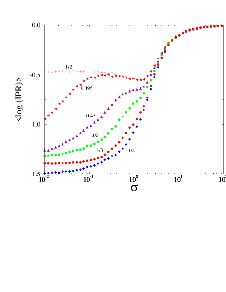
FIG. 11.: Variation of the averaged $\log$ (IPR) as a function of the disorder strength $\sigma$, for several values of $f$ ($N_{s}=605$ sites). The average is done over energies and over disorder realizations.

We first notice that, for $f=1/2$ the averaged IPR is indeed almost independent of $\sigma$ up to $\sigma\simeq 1$, in agreement with the qualitative picture given before. As $\sigma$ is further increased, the averaged IPR increases which is interpreted as a relative relocalization associated to an interband mixing. For $f<1/2$, another energy scale $D(f)$ related to the mean band width in absence of disorder emerges. If $\sigma<D(f)$, the localization length is finite for any $\sigma$ and decreases with $\sigma$ as indicated, for instance at $f=0.495$, by the corresponding increase of the IPR for low $\sigma$. This lasts until $D(f)\lesssim\sigma\lesssim 1$ where eigenstates no longer evolves with $\sigma$. The intermediate regime in smoothly connected to the plateau observed for $f=1/2$. It is, in some sense, what remains of Aharonov-Bohm cages as the field is no longer fixed to its special value $f=1/2$. Finally, the strong disorder regime ($\sigma\gtrsim 1$), where the localization length becomes comparable to the lattice spacing, is found not to depend sensitively of $f$ which sounds quite reasonable.

Similar conclusions can be drawn by looking at the density of states. Plots of this quantity at $f=1/2$ for various values of $\sigma$ are shown in Fig. 12. Note that the splitting of the three main peaks for $\sigma=0.01$ is due to edge states. The peaks broaden linearly with $\sigma$ in the plateau region which clearly ends when they merge.

Finally, we would like to mention a related study concerning the influence of the disorder on the transmission properties of quantum networks[12]. For sufficiently weak disorder, it has been shown that the periodicity with respect to the magnetic flux of the magnetoresistance remains equals to $h/e$ in the ${\cal T}_{3}$ lattice whereas it is completely dominated by the weak localization regime ($h/2e$) for more conventional structures, e. g. the square lattice. This indicates that the Aharonov-Bohm cages resists to a small amount of disorder. We emphasize that beautiful experiments by Naud et al. have recently shown up this phenomenon in two-dimensional electron gas (GaAs/GaAlAs)[11], measuring the magnetoresistance of mesoscopic artificial structures with the ${\cal T}_{3}$ geometry.

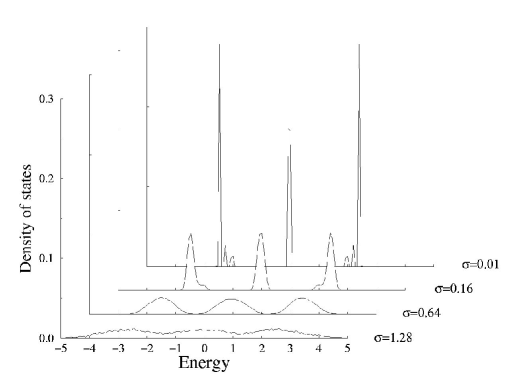
FIG. 12.: Variation of the averaged density of states at $f=1/2$ for various disorder strength $\sigma$ ($N_{s}=605$ sites).

V The edges states

As already mentioned, interesting edge state properties appear at $f=1/2$. We could study these states explicitely for the tight-binding hamiltonian $H_{0}$ but, for the sake of comparing with the experimental situations, we shall consider a continuous model where the network is made up of perfectly conducting one-dimensional wires. The Schrödinger equation for a free particle of mass $m$ moving along a wire reads :

$$-{\hbar^{2}\over 2m}{\mbox{d}^{2}\psi\over\mbox{d}x^{2}}=E\psi\mbox{ , }$$ (30)

where $x$ denotes the coordinate along the wire. For simplicity, we assume that no magnetic field is present but we will introduce it as soon as we will need it. If the extremities of the wire corresponds to nodes $i$ and $j$, and if the origin is chosen such that $x=0$ for node $i$ and $x=a$ for node $j$, we may write the general solution along the wire $(i,j)$ as :

$$\psi^{ij}(x)={1\over\sin(ka)}\left[\psi_{i}\sin(k(x-a))+\psi_{j}\sin(x)\right]\mbox{ ; }E(k)={\hbar^{2}k^{2}\over 2m}\mbox{ . }$$ (31)

For clarity, we have omit the index $k$, and we have set $\psi_{i}=\psi^{ij}(x=0)$ and $\psi_{j}=\psi^{ij}(x=a)$. The amplitudes on the nodes are constrained by a linear boundary conditions at each node of the network. A frequently used condition which is compatible with current conservation at the node $i$ is :

$$\sum_{\langle i,j\rangle}\left.{\mbox{d}\psi^{ij}(x)\over\mbox{d}x}\right|_{x=0}=0\mbox{ . }$$ (32)

Here, the sum is taken over the $z_{i}$ wires emerging from the node $i$. If we also impose the continuity condition of the wave function at each node ($\psi^{ij}(x=0)$ independent of $j$), we obtain the following set of equations :

$$\lambda z_{i}\psi_{i}=\sum_{\langle i,j\rangle}\psi_{j}\mbox{ . }$$ (33)

where we have introduced $\lambda=\cos ka$. So, a single value of $\lambda$ generates an infinite discrete family of eigenstates with energy $E(k_{n,\lambda})={\hbar^{2}\over 2m}\left(k_{\lambda}+{2\pi n\over a}\right)^{2}$ provided $\lambda=\cos k_{\lambda}a$. To describe each eigenstate only once, we may impose $k$ to lie in the interval $[-\pi/a,\pi/a]$. Note that Eq. (33) cannot be directly interpreted as an eigenvalue equation for a tight-binding problem since, in the general case, $z_{i}$ varies from one site to another. For an infinite ${\cal T}_{3}$ lattice, or a finite one with appropriate boundary conditions, the coordination number $z_{i}$ can only be equal to 3 or 6. It is therefore possible to perform the same decimation of the three fold-coordinated sites as for the tight-binding problem to obtain the same equation as Eq. (11) by setting $\varepsilon^{2}=18\lambda^{2}$. This simple correspondence between both problems also holds in the presence of a uniform magnetic field. In zero field, since $\varepsilon$ runs from $-\sqrt{18}$ to $\sqrt{18}$, $\lambda$ runs from $-1$ to $+1$ and therefore $k_{\lambda}$ from $[-\pi/a,\pi/a]$. So, there is no gap in the free electron spectrum on the network. As soon as the magnetic field is present, $k_{\lambda}$ has to be chosen from $[-\pi/a+\delta/a,-\delta/a]\cup[+\delta/a,\pi/a-\delta/a]$ where $\cos(\delta a)=\varepsilon_{max.}(f)/\sqrt{18}$, $\varepsilon_{max.}(f)$ denoting the largest eigenvalue of $H_{0}$ at reduced flux $f$. Thus, the free electron spectrum exhibits an infinite number of non overlapping bands, for generic $f$. Gaps in the spectrum have two different origins.Most of them corresponds to change the internal motion of the particle along a single link, which amounts to turn $n$ into $n+1$. Other gaps are induced by the magnetic field, and already appears as gaps in the set of allowed $\lambda$ values ($\lambda$ spectrum). For the special value $f=1/2$, the cage effect is manifested by the presence of a pure point-spectrum at energies $E_{n}={\hbar^{2}\over 2ma^{2}}\left(\pm\pi/2\pm\alpha+2\pi n\right)^{2}$, with $\alpha=\arcsin(1/\sqrt{3})$. Each of these levels is highly degenerate, reflecting all the possible cage states in the network.

Since some experiments have been performed on superconducting wire networks, it is worth recalling briefly the connection between the $\lambda$ spectrum and the estimate of the superconducting critical temperature as a function of the external flux $f$. At the transition, the order parameter builds up from the propagating modes of the linear Ginzburg-Landau equation (written here in zero field for simplicity) along each wire[6, 5] :

$$-{\mbox{d}^{2}\psi\over\mbox{d}x^{2}}+{1\over\xi^{2}}\psi=0\mbox{ . }$$ (34)

The critical temperature is obtained from the largest value of $\xi$ denoted by $\xi^{*}$, for which eigenvalues exist. $\xi^{*}$ is known as the Ginzburg-Landau macroscopic coherence length and we have $T_{c}(f)-T_{c}(0)\propto 1/(\xi^{*})^{2}$. To determine $\xi^{*}$, we follow the same procedure as for the free particle spectrum. We then have $(k^{*})^{2}=(\xi^{*})^{2}$ with $k^{*}\in[0,\pi/a]$ and $\cos(k^{*}a)=\lambda_{max.}(f)$. For an infinite lattice, one has : $\lambda_{max.}(f)=\varepsilon_{max.}(f)/\sqrt{18}$ so that the $T_{c}(f)$ curve is directly related to the edge of the tight-binding spectrum. This mapping has led to accurate comparisons between this simple model and the experimental data[8]. However, for free boundaries system, such a simple correspondence no longer holds, since the coordination number can be different from 3 and 6 on the edges. For these reasons, our discussion of edge states will be given mostly in term of the linear problem (33) rather than in the tight-binding language. The main striking result is the appearance of very sharp edge states at $f=1/2$. For those states, the amplitudes $\psi_{i}$’s are vanishing on most of the sites except on a finite width strip concentrated near the boundaries (see in Fig. 13).

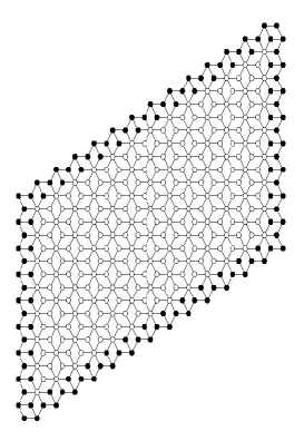
FIG. 13.: An example of edge states in a ${\cal T}_{3}$ wire network. We have put a black circle on each node for which the wave function has a non vanishing amplitude.

For any shape of the boundary, these edge states are always dispersive (along the edges). Note that in the tight-binding version, non dispersive edge states can also appear depending on the boundary shape. Another qualitative difference is that, in the tight-binding problem, the energy of these states always appears inside the main gaps of the infinite lattice spectrum whereas in the wire network, the $\lambda$ spectrum exhibits edge states with energy outside the bulk spectrum. We have displayed in Fig. 14 the spectrum of the finite lattice shown in Fig. 13 and the infinite lattice spectrum.

FIG. 14.: Comparison of the $\lambda$ spectrum for the infinite lattice (right) and the finite size lattice displayed in Fig. 13 (left).

The dispersive edge states are clearly visible. These have important consequences for superconducting networks since they offer the possibility to nucleate superconductivity on the edges of the sample, at temperatures slightly above the bulk $T_{c}(f)$[23, 24].

Notice that for specific boundaries, the dispersive edge states can run all around the sample as illustrated in Fig. 13, providing possibly an interesting example of a non chiral (quasi) one-dimensional conductor. Some experiments on ballistic networks etched in a two-dimensional electron gas in GaAs heterostructures have given some indications that edge states may have some influence in transport measurement[25]. Indeed, the variation of the conductance through such a ${\cal T}_{3}$ network with external field seems to depend on the geometry of the current pattern. On some samples, a stronger dip in the conductance at $f=1/2$ has been observed when the current is injected directly in the bulk, in comparison to the usual setup where the current is injected and collected on the edges. In this latter configuration, a non vanishing conductance may be found for a perfect system thanks to these propagating edge states[12]. For illustration, we give an analytical expression for edge states ($\lambda$ spectrum) coresponding to the semi-infinite ${\cal T}_{3}$ network displayed in Fig. 15. For these specific edges, the only non vanishing amplitudes are $A,C$ and $D$ ($B=0$). Therefore, we may choose a convenient gauge in the edge region as displayed in Fig. 15.

FIG. 15.: A possible edge choice for the semi-infinite ${\cal T}_{3}$ network (same convention as in Fig. 8).

Assuming propagating waves in the edge direction with wave vector $k$, we must satisfy the following set of equations :

$$3\lambda A = C+2D\cos(ka)$$ (35)

$$0 = 2C\cos(ka)-D$$ (36)

$$3\lambda C = A$$ (37)

$$3\lambda D = 2A\cos(ka)\mbox{ . }$$ (38)

The corresponding $\lambda$ spectrum is given by $\lambda=\pm{1\over 3}\sqrt{1+4\cos^{2}(ka)}$. This example shows a dispersive edge spectrum $\lambda\in[1/3,\sqrt{5}/3]$ that lies below and above $\lambda=1/\sqrt{3}$ which is the maximum value of $\lambda$ for the infinite system. As previously discussed, these states are thus more favourable than the bulk states for the nucleation of superconducting regions in a wire network upon cooling from high temperature.

We have also investigated how these very narrow edge states evolve as some perturbations away from the pure system at $f=1/2$ are gradually introduced. On Fig. 16, some edge states are represented for a pure system ($\sigma=0$) at $f=0.52$ and for a disordered system ($\sigma=0.01$) at $f=1/2$. Both cases are very similar. The main feature is the spatial broadening of the wave function towards the center of the sample. However, we observe a rather smooth evolution of these states as the strength of the perturbation is increased.

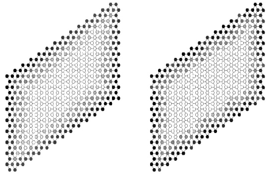
FIG. 16.: An example of edge states for $f=0.52,\sigma=0$ (left) and $f=1/2,\sigma=0.01$ (right). The grey level on site $i$ is proportional to the $\log|\psi_{i}|$.

Up to now, we have always consider that the electrons were independent. In the last section, we shall try to analyze the importance of the interactions between particles, in the ${\cal T}_{3}$ lattice. Note that for simpler systems, the two interacting particle problem under magnetic field has already revealed some unusual interesting features[26].

VI The interacting case

Of course, the many-body problem is certainly one of the most difficult to tackle. Here, our goal is to study, in a simple approach, the effect of the electron-electron interactions on the Aharonov-Bohm cages. We underline that this type of system provides a good starting point to understand the competition between localization and interaction even if the nature of the confinement is due to the magnetic field and not to disorder. In our case, the main departure from a realistic disordered model is indeed the preservation of the translation invariance in a localized system. In the following, we first focus on the two electron problem that already displays very interesting features, and we fix the reduced flux to its “critical value” $f=1/2$. The system is described by the following Hubbard hamiltonian :

$$H_{Hub.} = \sum_{\langle i,j\rangle,\sigma=\uparrow,\downarrow}t_{ij}\>c^{\dagger}_{i,\sigma}\,c_{j,\sigma}+U\sum_{i}n_{i,\uparrow}\,n_{i,\downarrow}$$ (39)

$$= H_{0}+H_{int.}\mbox{ , }$$ (40)

where $c^{\dagger}_{i,\sigma}$ and $c_{i,\sigma}$ denotes the creation and annihilation operator of a fermion with spin $\sigma$ respectively, $n_{i,\sigma}=c^{\dagger}_{i,\sigma}\,c_{i,\sigma}$ the density of spin $\sigma$ fermion on site $i$, and $\langle\ldots\rangle$ stands for nearest neighbor pairs. Note that, since the particles considered here are fermions, the interaction term $U$ is only efficient in the singlet sector where the orbital part of the wave function is symmetric. For simplicity, we completely neglect the coupling between the magnetic field and the electron spin.

Here, we shall mainly discuss the case of the ${\cal T}_{3}$ lattice but we must mention the work presented in ref.[14] on the chain of loops displayed in Fig. 9. For this system, we have shown that a Hubbard-like interaction term leads to a delocalization which is directly related to the emergence of dispersive bands in the two-particle spectrum. Of course, such a study is much more complex in the ${\cal T}_{3}$ lattice, but, as we shall see, it is however possible to show that the same effect is present in this two-dimensional structure.

First, let us remark that if, at a given time, both electrons are far from each other, the local particle density is non vanishing in a cage that is simply the superposition of each individual cages. The interesting case thus arises when the electrons get close. We consider, for instance, an initial state where both electrons $\uparrow$ and $\downarrow$ are located on the same six-fold coordinated site, and compute the coefficients of the recursion chain for this two-particle wave function. With the site numbering given in Fig. 4, we denote this initial state by $|\varphi_{0}\rangle=|0,0\rangle$. More generally, a ket $|i,j\rangle$ represents a state where the particle with spin $\uparrow$ is located on site $i$ and the particle with spin $\downarrow$ is located on site $j$. Note that we must, in principle, work with the symmetrized ket but, as shown below, since our initial ket $|0,0\rangle$ is already symmetric, it will automatically generate symmetrized kets. Applying the recursion algorithm in the gauge displayed in Fig. 17, one obtains :

$$H_{Hub.}|\varphi_{0}\rangle = U|0,0\rangle+\sum_{i=1}^{6}|i,0\rangle+|0,i\rangle$$ (41)

$$\Rightarrow\>\>\>a_{0} = U\,,\>b_{1}=2\sqrt{3}\,,\>|\varphi_{1}\rangle={1\over 2\sqrt{3}}\sum_{i=1}^{6}|i,0\rangle+|0,i\rangle\mbox{,}$$ (42)

$$H_{Hub.}|\varphi_{1}\rangle = {1\over\sqrt{3}}\sum_{i,j=1}^{6}|i,j\rangle+b_{1}|\varphi_{0}\rangle$$ (43)

$$\Rightarrow\>\>\>a_{1} = 0\,,\>b_{2}=2\sqrt{3}\,,\>|\varphi_{2}\rangle={1\over 6}\sum_{i,j=1}^{6}|i,j\rangle\mbox{,}$$ (44)

$$H_{Hub.}|\varphi_{2}\rangle = {U\over 6}\sum_{i=1}^{6}|i,i\rangle+b_{2}|\varphi_{1}\rangle$$ (45)

$$\Rightarrow\>\>\>a_{2} = {U\over 6}\,,\>b_{3}={U\sqrt{5}\over 6}\,,\>|\varphi_{3}\rangle={1\over\sqrt{5}}\left({5\over 6}\sum_{i=1}^{6}|i,i\rangle-{1\over 6}\sum_{i\neq j=1}^{6}|i,j\rangle\right)\mbox{,}$$ (46)

$$H_{Hub.}|\varphi_{3}\rangle = {1\over\sqrt{5}}\left({5\,U\over 6}\sum_{i=1}^{6}|i,i\rangle+\sum_{i=1}^{6}|i,i+6\rangle-|i,i+7\rangle+|i+6,i\rangle-|i+7,i\rangle\right)$$ (47)

$$\Rightarrow\>\>\>a_{3} = {5\,U\over 6}\,,\>b_{4}=2\,\sqrt{6\over 5}\,,\>|\varphi_{4}\rangle={1\over 2\sqrt{6}}\sum_{i=1}^{6}|i,i+6\rangle-|i,i+7\rangle+|i+6,i\rangle-|i+7,i\rangle\mbox{.}$$ (48)

Since $|\varphi_{4}\rangle$ has a non vanishing amplitude on the second shell sites ($i\geq 7$) the two-particle wave packet can spread, so that the Aharonov-Bohm cages associated to $|0,0\rangle$ seems to be unbound or, at least, larger than the one obtained for $|0\rangle$ at $U=0$. Actually, we have checked numerically that the $b_{i\geq 5}$’s are non vanishing so that the cage is really unbound.

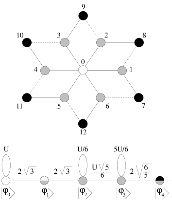
FIG. 17.: Aharanov-Bohm cage of a two-particle state initially localized on the central site, and its recursion chain (same convention as in Fig. 8). For $U\neq 0$, the black sites are reached.

As for the chain of loops, the propagation is made possible by the existence of two-body bound states in the spectrum. The same analysis as in ref.[14] could be done in the ${\cal T}_{3}$ lattice but the two-dimensional character of this later structure makes it more difficult. Nevertheless, if one focuses on the small interaction case ($U\ll t$) it is possible to show the emergence of dispersive bands near the ground state energy. Indeed, one can, in this case, treat $U$ as a perturbation on the infinitely degenerate level $2\varepsilon_{-}$ without considering the higher energy levels.

To solve this problem, we shall use the periodic gauge displayed in Fig. 18 that provides real hopping terms.

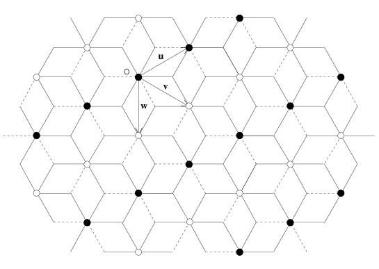
FIG. 18.: A possible gauge choice for the ${\cal T}_{3}$ lattice at $f=1/2$ (same convention as in Fig. 8).

Remark that the periodicity of the structure has doubled and we must now distinguish two different types of 6-fold coordinated sites denoted by $(\bullet)$ and $(\circ)$. If one restricts the two-body problem analysis to the subspace corresponding to $2\varepsilon_{-}$ (for $U=0$), it is convenient to build the two-particle state basis as the tensor product of the one-particle orthogonal “cage” basis displayed in Fig. 19.

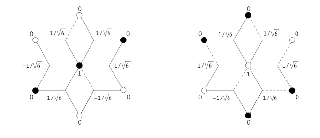
FIG. 19.: Non-normalized one-particle cage eigenstates associated to the two types of 6-fold coordinated sites (see Fig. 18). The amplitude on each site is given.

Since the problem is invariant under a translation of the center of mass of the two particles, the basis of the singlet states sensitive to $U$ can be expressed in terms of the following Bloch waves :

$$|\varphi_{0}({\bf K})\rangle = {1\over\sqrt{N_{s}}}\sum_{{\bf r}\in\Lambda}e^{i{\bf K.r}}|{\bf r},{\bf r}\rangle$$ (49)

$$|\varphi_{1}({\bf K})\rangle = {1\over\sqrt{N_{s}}}\sum_{{\bf r}\in\Lambda}e^{i{\bf K.r}}|{\bf r+v},{\bf r+v}\rangle$$ (50)

$$|\varphi_{\bf u_{0}}({\bf K})\rangle = {1\over\sqrt{N_{s}}}\sum_{{\bf r}\in\Lambda}e^{i{\bf K.r}}|{\bf r},{\bf r+u}\rangle_{S}$$ (51)

$$|\varphi_{\bf u_{1}}({\bf K})\rangle = {1\over\sqrt{N_{s}}}\sum_{{\bf r}\in\Lambda}e^{i{\bf K.r}}|{\bf r+v},{\bf r+v+u}\rangle_{S}$$ (52)

$$|\varphi_{\bf\pm v}({\bf K})\rangle = {1\over\sqrt{N_{s}}}\sum_{{\bf r}\in\Lambda}e^{i{\bf K.r}}|{\bf r},{\bf r\pm v}\rangle_{S}$$ (53)

$$|\varphi_{\bf\pm w}({\bf K})\rangle = {1\over\sqrt{N_{s}}}\sum_{{\bf r}\in\Lambda}e^{i{\bf K.r}}|{\bf r},{\bf r\pm w}\rangle_{S}\mbox{,}$$ (54)

where the origin $O=(0,0)$, ${\bf u}$, ${\bf v}$ and ${\bf w}$ are represented in Fig. 18 ; $\Lambda$ is the lattice generated by ${\bf u}$ and ${\bf v+w}$ with periodic boundary conditions and containing $N_{s}$ sites ; ${\bf K}$ is a wave vector lying in the first Brillouin zone associated to $\Lambda$. Note that the orthogonal basis used here to define the different vectors is different than the basis used in section III. From now on, the ket $|{\bf r},{\bf r^{\prime}}\rangle_{S}$ represents the normalized space symmetric state in which one electron is in a cage state (eigenstate of the one-particle non interacting problem) localized around a six-fold coordinated site located in ${\bf r}$ and the other electron is in a cage state localized around a six-fold coordinated site located in ${\bf r}^{\prime}$. Because of the Pauli principle, these kets corresponds to antisymmetric spin wave functions and therefore to singlet states. Note that $|{\bf r};{\bf r}\rangle$ is automatically symmetric so that we have omit the index $S$ for this state. Naturally, if $|{\bf r}-{\bf r}^{\prime}|>\sqrt{3}$, the electrons do not interact so that one may only to consider the 8 two-particle states defined above. Thus, in each irreducible representation indexed by ${\bf K}$, one just has to diagonalize $H_{Hub.}$ in the subspace generated by these vectors. Furthermore, as shown in the Appendix A, $H_{Hub.}$ can be block diagonalized into two isospectral matrices. After shifting the energies so that for $U=0$ the eigenenergies are equal to zero (and not to $2\varepsilon_{-}$), the eigenvalues (in $U$ units) are given by the roots of the following characteristic polynomial :

$$P(\varepsilon,{\bf K})=\varepsilon[10368\varepsilon^{3}-\varepsilon^{2}(3888+288\mu)+\varepsilon(258+20\mu+2\nu)+\mu-3]\mbox{.}$$ (55)

$$\mu = \cos({\bf K}.{\bf u})+\cos({\bf K}.{\bf v})+\cos({\bf K}.{\bf w})$$ (56)

$$\nu = \cos[{\bf K}.{\bf(u+v)}]+\cos[{\bf K}.{\bf(2u-v})]+\cos[{\bf K}.{\bf(2v-u})]\mbox{.}$$ (57)

Reminding that ${\bf w}={\bf v}-{\bf u}$, one can easily check that $P$ is unchanged by the tranformation ${\bf u}\leftrightarrow{\bf v}$, as it obviously should.

It is readily seen in Eq.(55) that $\varepsilon=0$ is always an eigenvalue for all ${\bf K}$. The associated eigenvectors have a vanishing amplitude on the kets $|\varphi_{0}({\bf K})\rangle$ and $|\varphi_{1}({\bf K})\rangle$ that corresponds to states where both electrons are in the same cage. The absence of dispersion for this family of states suggests that they may be generated by a set localized two particle singlets. As in the one particle problem (see Section III), it is even possible to exhibit such states where the center of mass is confined in a finite area. A possible choice is :

$$|\psi_{Bound}\rangle={1\over\sqrt{6}}\left(|{\bf 0},{\bf u}\rangle_{S}-|{\bf 0},-{\bf u}\rangle_{S}-|{\bf 0},{\bf v}\rangle_{S}+|{\bf 0},-{\bf v}\rangle_{S}+|{\bf 0},{\bf w}\rangle_{S}+|{\bf 0},-{\bf w}\rangle_{S}\right)$$ (58)

The presence of these localized singlet bound states at zero energy seems to be a particular feature of this lattice.

Apart from this non dispersive band, a close inspection of the polynomial $P$ allows one to show that when ${\bf K}$ runs over an elementary cell of the reciprocal lattice, the roots of $P$ describe two separate dispersive bands spreading from 0 to 1/12 for the lower one and from 1/4 to 3/8. The corresponding eigenvectors are linear combinations of the 8 vectors introduced above and are actually extended Bloch waves. These two-body bound states are delocalized and thus allow for a propagation of two-particle wave functions as we have already noticed using the recursion analysis (see in Fig. 17). The same perturbative approach in the degenerate ground state can be achieved for the chain of loops[14]. In this latter case, the spectrum, for $U\ll t$ consists in two non dispersive bands with eigenenergies 0 and 1/16, and one dispersive band spreading also from $1/4$ to $3/8$. Here again these energies are measured in $U$ units and shifted such that, for $U=0$, the two-body ground state corresponds to a zero energy. We have displayed in Fig. 20 these two spectra.

Two important differences arise between these two structures. First, there is no non dispersive singlet bound state at zero energy for the chain of loops, except the trivial ones involving two remote localized electron states. Non dispersive singlet bound states do exist but their energy is strictly positive and depends on $U$. Second, there is a gap between the $U=0$ ground state and the first dispersive band (bound state), by contrast to the ${\cal T}_{3}$ lattice.

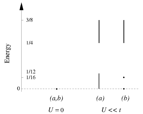
FIG. 20.: Perturbative low-energy two-particle spectrum for $(a)$ the ${\cal T}_{3}$ lattice, $(b)$ the chain of loops.

The fact that all eigenenergies of the projected hamiltonian are positive is a simple consequence of the same property for the interacting part $H_{int.}$. Denoting by $Q$ the projector on the lowest energy level of $H_{0}$, the lowest order degenerate perturbation theory proposed above amounts to diagonalize $QH_{int.}Q$. For any two-particle eigenstate $|\psi\rangle$, we have $\langle\psi|H_{int.}|\psi\rangle\geq 0$ if $U\geq 0$. In particular, this imposes all eigenvalues of $QH_{int.}Q$ to be positive (or vanishing). From this consideration, the appearance of non trivial (degenerate) zero energy bound states in the singlet sector is quite remarkable.

Of course, it would be very interesting to characterize the properties of the system in the presence of a finite density of particles. In the following discussion, we shall always assume $U\ll t$, so that we will only pay attention to the projected hamiltonian $QH_{int.}Q$ which is, as discussed above, a positive operator. Denoting by $N_{e}$ the total number of electrons and by $N_{s}$ the total number of sites, we introduce the density $\rho=N_{e}/N_{s}$ that ranges from 0 to 2 because of the spin degeneracy. In the non interacting case, for $0\leq\rho\leq 2/3$, it is possible to put all the electrons, in the ground state of $H_{0}$. Thus, we will restrict our analysis to this interval.

For $\rho\leq 1/3$, a possible choice for the ground state is to put each electron in a localized cage state (around 6-fold coordinated sites). In this case, the energy per particle is simply $\varepsilon_{-}$. At low density, if all occupied cages are further isolated from each other (no overlap), the interaction term $H_{int.}$ does not affect these configurations which are therefore ground states of $QH_{Hub.}Q$. These configurations have a huge spin degeneracy ($2^{N_{e}}$). One can also build ground state configurations containing some connected clusters of singly occupied cage states, provided these clusters are fully spin polarized. Obviously, the total spins of these clusters may be chosen independently from each other without any energy cost. Note that additional configurations with the same energy may also be obtained using the zero energy two particle localized singlet bound states discussed above. An interesting issue would be to determine whether this class of ground states exhausts all the possible ones, for $\rho\leq 1/3$. Note that if the density $\rho$ lies beyond $\nu_{T}/3$ where $\nu_{T}$ is the site percolation density of the triangular lattice which is formed by the 6-fold coordinated sites, we have an infinite percolating cluster which leads to an infinite magnetization.

As $\rho$ approaches $1/3$, the ground state thus becomes more and more polarized. If $N_{s}$ denotes the total number of sites, the problem of finding the ground state of the projected hamiltonian becomes more interesting if $1/3<\rho\leq 2/3$. A simple class of eigenstates of $QH_{Hub.}Q$ is obtained if the magnetization is maximal. It corresponds to a total spin $S_{max.}=N_{s}/3-N_{e}/2$. Indeed, because of the spin rotation invariance, such states can be built from states with $N_{\uparrow}=N_{s}/3$ and $N_{\downarrow}=N_{e}/2-N_{s}/3$ after performing a global spin rotation. Here, $N_{\uparrow}$ and $N_{\downarrow}$ denotes the total number of electrons with up and down spins respectively. The condition $N_{\uparrow}=N_{s}/3$ means that all the single particle ground states of $H_{0}$ are fully occupied by $\uparrow$ spin electrons. For these states, the $\downarrow$ spin electrons behave as completely localized free fermions with an individual excitation energy equal to $U$. To show this, we denote by $\varphi_{\bf r}(i)=\langle i|{\bf r}\rangle$ the amplitude at site $i$ of the state $|{\bf r}\rangle$ which is the single particle cage eigenstates of $H_{0}$ localized around the six-fold coordinated site located at site ${\bf r}$, and we write :

$$QH_{int.}Q=\sum_{{\bf r}_{1},{\bf r}_{2},{\bf r}_{3},{\bf r}_{4}}u({\bf r}_{3},{\bf r}_{4}|{\bf r}_{1},{\bf r}_{2})\>\>c^{\dagger}_{{\bf r}_{3},\uparrow}c^{\dagger}_{{\bf r}_{4},\downarrow}c_{{\bf r}_{2},\downarrow}c_{{\bf r}_{1},\uparrow}\mbox{,}$$ (59)

with :

$$u({\bf r}_{3},{\bf r}_{4}|{\bf r}_{1},{\bf r}_{2})=U\sum_{j}\varphi^{*}_{{\bf r}_{3}}(j)\varphi^{*}_{{\bf r}_{4}}(j)\varphi_{{\bf r}_{2}}(j)\varphi_{{\bf r}_{1}}(j)\mbox{.}$$ (60)

In expression (59), the fermions operator $c^{\dagger}_{{\bf r},\sigma}$ and $c_{{\bf r},\sigma}$ create and destroy an electron with spin $\sigma$ in a state $|{\bf r}\rangle$. On a state where all the single particle ground states of $H_{0}$ are fully occupied by up spins electrons, $c^{\dagger}_{{\bf r}_{3},\uparrow}c_{{\bf r}_{1},\uparrow}$ acts as $\delta_{{\bf r}_{3},{\bf r}_{1}}$ times the identity operator. It is then easy to check that : $\sum_{{\bf r}}u({\bf r}_{,}{\bf r}_{4}|{\bf r},{\bf r}_{2})=U\delta_{{\bf r}_{4},{\bf r}_{2}}$. As a consequence, for any state $|\psi\rangle$ such that $N_{\uparrow}=N_{s}/3$, we have $QH_{int.}Q|\psi\rangle=UN_{\downarrow}|\psi\rangle$. At this stage, it not clear whether the ground state of the projected hamiltonian has the maximal value $S_{max.}$ of the total spin for $1/3<\rho\leq 2/3$. Nevertheless, since this is true for $\rho=1/3$ according to the previous paragraph, this generalization is plausible. The main question to be adressed is whether a $\downarrow$ spin may form a bound state with one or several “magnons”. By magnon, we refer here to particle-hole like excitations which destroy one $\uparrow$ spin electron and create one $\downarrow$ spin electron. We leave this interesting but more complex problem for future investigations.

To conclude this section, we may say that in spite of the presence of very low lying dispersive bound states for two particles, it is not so easy to turn the finite density system into a good conductor. However, we emphasize that some qualitative changes may arise for finite values of $U$, since a sizeable virtual occupancy of excited levels of $H_{0}$ becomes then possible.

VII Conclusion and perspectives

In this paper, we have studied three types of perturbations which affect the physical properties of a two-dimensional lattice embedded in a magnetic field that presents Aharonov-Bohm cages. Two of them, namely a weak Anderson-like disorder and the finite size effects do not drastically modify the main features of the ideal model. In particular, if the disorder is not too important, the single particle energy eigenstates remain strongly localized for half-integer fluxes per elementary tile, and this independently of the disorder strength. This lasts until the disorder does not introduce a strong mixing between distinct degenerate levels of the unperturbed tight-binding hamiltonian. By contrast, for generic values of the magnetic field, the amount of disorder-induced localization is very sensitive to the disorder strength.

A more delicate situation is obtained in the presence of electron-electron interactions for the many-body system. We have shown how they partially destroy the single particle localization by the generation of extended two particle eigenstates. However, it is not clear at the present stage whether this mechanism is sufficient to induce a metallic behavior for finite electron densities and half a flux quantum per tile. This important question clearly deserves further investigations for the Hubbard model (studied here) and also for more realistic model of continuous narrow wires (few conducting channels), in connection to the experiments on two-dimensional electron gas. We expect to find partially spin polarized ground states in a finite interval of electron density, and a fully polarized state when the number of electron per site equals $1/3$. For slightly larger densities, an important question is to understand if the system create some spin textures resembling to skyrmions in quantum Hall effect for filling fractions close to odd integers.

In this context, it would be very interesting to study interacting hard core bosons on this lattice, which would require numerical diagonalization on finite size clusters. Indeed, this model is closely related to the physics of Josephson junction arrays. In the limit of small capacitance islands quantum fluctuations of the order parameter phase are strong and the corresponding trend to localize Cooper pairs could be enhanced by the cage effect. In the other limit where the Josephson coupling dominates, it is not clear that the system at half-integer fluxes will develop a finite stiffness for spatial gradients of the order parameter phase. In this semi-classical regime, we expect a rather large ground state degeneracy as suggested by vortex decoration experiments on superconducting networks.

A Diagonalization of the two-electron problem

As explained in section VI, the non trivial part of the hamiltonian is given, in each irreducible representation indexed by ${\bf K}$, by the subspace generated by the eight vectors :

$$\left(|\varphi_{0}({\bf K})\rangle,|\varphi_{\bf+v}({\bf K})\rangle,|\varphi_{\bf-v}({\bf K})\rangle|\varphi_{\bf u_{0}}({\bf K})\rangle,|\varphi_{\bf u_{1}}({\bf K})\rangle,|\varphi_{\bf+w}({\bf K})\rangle,|\varphi_{\bf-w}({\bf K})\rangle,\varphi_{1}({\bf K})\rangle\right).$$

In this basis, the shifted hamiltonian $H^{\prime}({\bf K})=(H_{Hub.}({\bf K})-2\varepsilon_{-}I_{8})/U$ ($I_{8}$ denotes the $8\times 8$ identity matrix) writes :

$$H^{\prime}({\bf K})=\left(\begin{array}[]{cccccccc}{7\over 24}+{\cos({\bf K}.{\bf u})\over 36}&{e^{-i{\bf K}.{\bf u}}\over 72\sqrt{2}}&-{e^{i{\bf K}.{\bf u}}\over 72\sqrt{2}}&0&{e^{-i{\bf K}.{\bf u}}-e^{-2i{\bf K}.{\bf v}}\over 72\sqrt{2}}&{e^{i{\bf K}.{\bf u}}\over 72\sqrt{2}}&{e^{-i{\bf K}.{\bf u}}\over 72\sqrt{2}}&{e^{-i{\bf K}.{\bf v}}(\cos({\bf K}.{\bf v})+\cos({\bf K}.{\bf w}))\over 36}\\ \\ &{1\over 36}&0&{1\over 72}&-{e^{-i{\bf K}.{\bf u}}\over 72}&{1+e^{i{\bf K}.{\bf u}}\over 72}&0&-{e^{-i{\bf K}.{\bf u}}\over 72\sqrt{2}}\\ \\ &&{1\over 36}&{e^{-i{\bf K}.{\bf u}}\over 72}&-{e^{-2i{\bf K}.{\bf v}}\over 72}&0&{-1-e^{-i{\bf K}.{\bf u}}\over 72}&{e^{-i{\bf K}.{\bf(v+w)}}\over 72\sqrt{2}}\\ \\ &&&{1\over 36}&0&{e^{i{\bf K}.{\bf u}}\over 72}&-{1\over 72}&{1-e^{-i{\bf K}.{\bf(v+w)}}\over 72\sqrt{2}}\\ \\ &&&&{1\over 36}&-{e^{i{\bf K}.{\bf u}}\over 72}&{e^{2i{\bf K}.{\bf v}}\over 72}&0\\ \\ &&&&&{1\over 36}&0&{-1\over 72\sqrt{2}}\\ \\ &&&&&&{1\over 36}&{-e^{-2i{\bf K}.{\bf v}}\over 72\sqrt{2}}\\ \\ &&&&&&&{7\over 24}+{\cos({\bf K}.{\bf u})\over 36}\end{array}\right)\mbox{ . }$$ (A1)

Note that since $H^{\prime}({\bf K})$ is hermitian, we have only given its upper part. Now, let us introduce the following vectors :

$$|\varphi({\bf K})\rangle_{\pm} = {1\over\sqrt{2}}\left(|\varphi_{0}({\bf K})\rangle\pm e^{-i{\bf K.v}}|\varphi_{1}({\bf K})\rangle\right)$$ (A2)

$$|\varphi_{\bf u}({\bf K})\rangle_{\pm} = {1\over\sqrt{2}}\left(|\varphi_{\bf u_{0}}({\bf K})\rangle\pm e^{-i{\bf K.v}}|\varphi_{\bf u_{1}}({\bf K})\rangle\right)$$ (A3)

$$|\varphi_{\bf v}({\bf K})\rangle_{\pm} = {1\over\sqrt{2}}\left(|\varphi_{\bf+v}({\bf K})\rangle\pm e^{i{\bf K.v}}|\varphi_{\bf-v}({\bf K})\rangle\right)$$ (A4)

$$|\varphi_{\bf w}({\bf K})\rangle_{\pm} = {1\over\sqrt{2}}\left(|\varphi_{\bf+w}({\bf K})\rangle\pm e^{i{\bf K.w}}|\varphi_{\bf-w}({\bf K})\rangle\right)\mbox{,}$$ (A5)

that corresponds (up to a phase factor), to symmetric and antisymmetric combinations of the initials vectors. The hamiltonian does not connect the subspace generated by ${\cal B}_{1}=(|\varphi({\bf K})\rangle_{-},|\varphi_{\bf v}({\bf K})\rangle_{-}|\varphi_{\bf u}({\bf K})\rangle_{+},|\varphi_{\bf w}({\bf K})\rangle_{+})$ and the subspace generated by ${\cal B}_{2}=(|\varphi({\bf K})\rangle_{+},|\varphi_{\bf v}({\bf K})\rangle_{+},|\varphi_{\bf u}({\bf K})\rangle_{-},|\varphi_{\bf w}({\bf K})\rangle_{-})$. In each subpace, $H^{\prime}({\bf K})$ writes :

$$H^{\prime}_{{\cal B}_{1}}({\bf K})=\left(\begin{array}[]{cccc}{7\over 24}+{\cos({\bf K}.{\bf u})+\cos({\bf K}.{\bf v})+\cos({\bf K}.{\bf w})\over 36}&{e^{-i{\bf K.u}}-e^{-i{\bf K.w}}\over 72\sqrt{2}}&{e^{-i{\bf K.u}}-e^{-2i{\bf K.v}}\over 72\sqrt{2}}&{e^{-i{\bf K.u}}-e^{i{\bf K.v}}\over 72\sqrt{2}}\\ \\ &{1\over 36}&{-e^{-i{\bf K.u}}-e^{-i{\bf K.v}}\over 72}&{-e^{i{\bf K.v}}-e^{i{\bf K.w}}\over 72}\\ \\ &&{1\over 36}&{e^{i{\bf K.v}}+e^{2i{\bf K.v}}\over 72}\\ \\ &&&{1\over 36}\end{array}\right)\mbox{ , }$$ (A6)

$$H^{\prime}_{{\cal B}_{2}}({\bf K})=\left(\begin{array}[]{cccc}{7\over 24}+{\cos({\bf K}.{\bf u})-\cos({\bf K}.{\bf v})-\cos({\bf K}.{\bf w})\over 36}&{e^{i{\bf K.(u+v)}}+e^{-i{\bf K.(v+w)}}\over 72\sqrt{2}}&{1-e^{i{\bf K.(v+w)}}\over 72\sqrt{2}}&{-1-e^{i{\bf K.(u+v)}}\over 72\sqrt{2}}\\ \\ &{1\over 36}&{e^{-i{\bf K.u}}-e^{-i{\bf K.v}}\over 72}&{-e^{-i{\bf K.v}}-e^{-i{\bf K.w}}\over 72}\\ \\ &&{1\over 36}&{e^{-i{\bf K.u}}-e^{-i{\bf K.w}}\over 72}\\ \\ &&&{1\over 36}\end{array}\right)\mbox{ . }$$ (A7)

The characteristic polynomia $P_{{\cal B}_{1}}(\varepsilon,{\bf K})$ and $P_{{\cal B}_{2}}(\varepsilon,{\bf K})$ associated to $H^{\prime}_{{\cal B}_{1}}({\bf K})$ and $H^{\prime}_{{\cal B}_{2}}({\bf K})$ respectively reads :

$$P_{{\cal B}_{1}}(\varepsilon,{\bf K}) = {\varepsilon\over 10368}[10368\varepsilon^{3}-\varepsilon^{2}(3888+288\mu_{1})+\varepsilon(258+20\mu_{1}+2\nu_{1})+\mu_{1}-3]$$ (A8)

$$P_{{\cal B}_{2}}(\varepsilon,{\bf K}) = {\varepsilon\over 10368}[10368\varepsilon^{3}-\varepsilon^{2}(3888+288\mu_{2})+\varepsilon(258+20\mu_{2}+2\nu_{2})+\mu_{2}-3]\mbox{,}$$ (A9)

with :

$$\mu_{1} = \cos({\bf K}.{\bf u})+\cos({\bf K}.{\bf v})+\cos({\bf K}.{\bf w})$$ (A10)

$$\mu_{2} = \cos({\bf K}.{\bf u})-\cos({\bf K}.{\bf v})-\cos({\bf K}.{\bf w})$$ (A11)

$$\nu_{1} = \cos[{\bf K}.{\bf(u+v)}]+\cos[{\bf K}.{\bf(2u-v})]+\cos[{\bf K}.{\bf(2v-u})]$$ (A12)

$$\nu_{2} = -\cos[{\bf K}.{\bf(u+v)}]-\cos[{\bf K}.{\bf(2u-v})]+\cos[{\bf K}.{\bf(2v-u})]\mbox{ . }$$ (A13)

In the orthogonal basis chosen in section II where ${\bf u}=a(3/2,\sqrt{3}/2)$, ${\bf v}=a(3/2,-\sqrt{3}/2)$ and ${\bf w}={\bf v}-{\bf u}$, it is straightforward to show that $P_{{\cal B}_{1}}(\varepsilon,{\bf K})=P_{{\cal B}_{2}}(\varepsilon,{\bf K^{\prime}})$ if ${\bf K}=(k_{1},k_{2})$ and ${\bf K^{\prime}}=(k_{1}+\pi/3,k_{2}-\pi/\sqrt{3})$. Thus, it is sufficient to analyze the roots of the polynomial $P(\varepsilon,{\bf K})=P_{{\cal B}_{1}}(\varepsilon,{\bf K})$ for all ${\bf K}$ belonging to an elementary cell of the reciprocal lattice.

REFERENCES

- [1] M. Y. Azbel, Sov. Phys. JETP 19, 634 (1964).
- [2] D. Hofstadter, Phys. Rev. B 14, 2239 (1976).
- [3] F. H. Claro and G. H. Wannier, Phys. Rev. B 19, 6068 (1979).
- [4] R. Rammal, J. Phys. (Paris) 46, 1345 (1985).
- [5] P. G. de Gennes, C. R. Acad. Sci. Ser. B 292 9 and 279 (1981).
- [6] S. Alexander, Phys. Rev. B 27, 1541 (1983).
- [7] J. Vidal, R. Mosseri, and B. Douçot, Phys. Rev. Lett. 81, 5888 (1998).
- [8] C. C. Abilio et al., Phys. Rev. Lett. 83, 5102 (1999).
- [9] E. Serret et al., in preparation.
- [10] B. Pannetier et al., cond-mat/0005254.
- [11] C. Naud, G. Faini, and D. Mailly, cond-mat/0006400.
- [12] J. Vidal, G. Montambaux, and B. Douçot, Phys. Rev. B 62, 16294 (2000).
- [13] R. B Laughlin, Phys. Rev. Lett. 50, 1395 (1983).
- [14] J. Vidal, B. Douçot, R. Mosseri, and P. Butaud, Phys. Rev. Lett. 85, 3906 (2000).
- [15] D. L. Shepelyansky, Phys. Rev. Lett. 73, 2607 (1994).
- [16] D. N. Basov et al., J. Math. Phys. 11, 784 (1970).
- [17] R. E. Peierls, Z. Phys. 80, 763 (1933).
- [18] B. Sutherland, Phys. Rev. B 34, 5208 (1986).
- [19] R. Haydock, V. Heine, and M. J. Kelly, J. Phys. C 5, 2845 (1972), and ibid 8, 2591 (1975).
- [20] R. Ketzmerick, G. Petschel, and T. Geisel, Phys. Rev. Lett. 69, 695 (1992).
- [21] G. Y. Oh, Phys. Rev. B 62, 4567 (2000).
- [22] V. Elser, Phys. Rev. Lett. 54, 1730 (1985).
- [23] P. G. de Gennes, Superconductivity of Metals and Alloys (W. A. Benjamin, New York, 1966).
- [24] A. Bezryadin, Y. N. Ovchinnikov, and B. Pannetier, Phys. Rev. B 53, 8553 (1996).
- [25] C. Naud, G. Faini, and D. Mailly, in preparation.
- [26] A. Barelli, J. Bellissard, P. Jacquod, and D. L. Shepelyansky, Phys. Rev. Lett. 77, 4752 (1996).