The 2-site Hubbard and $t$-$J$ models

Abstract

The fermionic and bosonic sectors of the 2-site Hubbard model have been exactly solved by means of the equation of motion and Green’s function formalism. The exact solution of the $t$-$J$ model has been also reported to investigate the low-energy dynamics. We have successfully searched for the exact eigenoperators, and the corresponding eigenenergies, having in mind the possibility to use them as an operatorial basis on the lattice. Many local, single-particle, thermodynamical and response properties have been studied as functions of the external parameters and compared between the two models and with some numerical and exact results. It has been shown that the 2-site Hubbard model already contains the most relevant energy scales of the Hubbard model: the local Coulomb interaction $U$ and the spin-exchange one $J=\frac{4t^{2}}{U}$. As a consequence of this, for some relevant properties (kinetic energy, double occupancy, energy, specific heat and entropy) and as regards the metal-insulator transition issue, it has resulted possible to almost exactly mime the behavior of larger systems, sometimes using a higher temperature to get a comparable level spacing. The 2-site models have been also used as toy models to test the efficiency of the Green’s function formalism for composite operators. The capability to reproduce the exact solutions, obtained by the exact diagonalization technique, gives a firm ground to the approximate treatments based on this formalism.

I Introduction

Two are the aspects that gave so much popularity to the Hubbard model: the richness of its dynamics that is thought to permit a description of many puzzling issues like metal-insulator transition, itinerant magnetism, electronic superconductivity, and the simplicity of the Hamiltonian structure that let one speculate about the possibility of finding the exact and complete solution for any realization of the underlying lattice. Anyway, although the model has been studied more than any other one in the last fifty years, very few exact results are available and what we have mainly regards either finite clusters or the infinite chain (i.e., the 1D case). For finite clusters of 2Harris and Lange (1967); Shiba and Pincus (1972) or 4Shiba and Pincus (1972); Heinig and Monecke (1972a, b); Cabib and Kaplan (1973); Schumann (2002) sites it is possible to find the complete set of eigenstates and eigenvalues of the Hamiltonian and compute any quantity by means of the thermal averages. However, it is not easy at all, although possible in principle, to extract valuable and scalable (i.e., which can be used to find the solutions of bigger and bigger clusters and, ultimately, of the infinite lattice cases) information regarding the effective excitations present in the system, the operators describing them and their dynamics. For the infinite chain neither, we have all the information we wish; the Bethe Ansatz is a very powerful tool, but is severely limited as regards the range of applicability of the self-consistent equations it supplies and the quantities for which it gives an answer.

In this manuscript, in order to overcome the limitations discussed above, we have exactly solved the Hubbard model, on a 2-site cluster, completely within the equations of motion and the Green’s function formalism. By using this approach, we have had the possibility to find the complete set of eigenoperators of the Hamiltonian and the corresponding eigenenergies. This information has been really fundamental as it permitted a deeper comprehension of the features shown by the properties we have analyzed. It is worth noting that the Hubbard model on a 2-site cluster is the smallest system where both terms of the Hamiltonian (i.e., kinetic and electrostatic) are effective and contributes to the dynamics.

By properly tuning the value of the temperature, we have found that the 2-site system can almost perfectly mime, as regards relevant properties such as the kinetic energy, the double occupancy, the energy, the specific heat, the entropy and fundamental issues such as the metal insulator transition, the behavior of larger clusters and of the infinite chain. The tuning of the temperature is necessary in order to get a comparable effective level spacing (bigger the cluster, lower the spacing), i.e. to excite the correct levels: the relevant energy scales are present although the relative positions of the levels are affected by the size of the system (only two k points!). The very positive comparisons with exact results (Bethe Ansatz, exact diagonalization) and numerical data (quantum Monte Carlo, Lanczos) support the idea that a lot of physics can be described and understood within this very small system, for which there is the possibility to know the analytic expressions for all the quantities under study. As regards the relevant scales of energy, this 2-site system has demonstrated to contain all the necessary ingredients to describe many features coming from the strong electronic correlations and also appearing in the lattice case. Two of the three relevant energy scales, which are thought to be present in the Hubbard model, naturally emerge: the local Coulomb interaction $U$ and the spin-exchange one $J=\frac{4t^{2}}{U}$ that is, in principle, extraneous to the original purely electrostatic Hamiltonian and is dynamically generated by the combined actions of the two terms of the Hamiltonian. As useful guide to better understand the low-energy dynamics we have also solved the $t$-$J$ model and presented the solution in parallel with the one found for the Hubbard model.

This analysis, which have resulted to be really relevant by itself as we have got a much better understanding of some energy scales and internal parameter dynamics, has been worth to be performed also as a prelude of the lattice analysis. In fact, the eigenoperators we have found, both in the fermionic and the bosonic sectors, can be used in the lattice case as a basis for the Green’s functions. In the strongly correlated systems, the interactions can alter so radically the dynamics of the original particles that these latter lose completely their own identitiesUmezawa (1993). Actually, some new objects are generated by the interactions and dictate the physical response. They are not so easy to be identified: their number, exact expression and relevance can only be suggested by the experience and, when available, by exact and/or numerical results. For instance, one can choose: the higher order fields emerging from the equations of motion, the eigenoperators of some relevant interacting terms, the eigenoperators of the problem reduced to a small cluster, etc. In the last years, we have been focusing our activity on the study of strongly correlated electronic models like Kondo, $t$-$J$, $p$-$d$, Hubbard by means of the Composite Operator MethodCOM (a, b); Mancini (1998); Fiorentino:00a; Mancini and Avella (2003) that is based on two main ideas: one is the use of composite fields as basis for our Green’s functions, in accordance to what has been discussed above, and the other one is the exploitation of algebra constraints (e.g., the Pauli principle, the particle-hole symmetry, the Ward-Takahashi identities, …) to fix the correct representation of the Green’s functions and to recover the links among the spin and charge configurations dictated by the symmetries. It is worth noticing that the Composite Operator Method is exact in itself. An additional approximation treatment is needed when we deal with large or infinite degree-of-freedom systems; in this case we have to treat in an approximate way the otherwise intractable hierarchy of the equations of motion generated by the projection procedure. If no approximation is necessary (finite and reasonably small degree-of-freedom systems), the COM cannot do else than give the exact solution. According to this, the COM gives the exact solution also for the two systems under analysis in this manuscript: the two-site Hubbard and t-J models. Whenever, instead, we should resort to an approximate treatment to close the hierarchy of the equations of motion generated by the projection procedure, we expect some limitations connected with the chosen approximation. For instance, we get only the first moments correct if we truncate the equations of motion hierarchy Mancini (1998). On the other hand, it is really worth noting that we properly take into account: the interaction term of the Hamiltonian by using as basis operators its eigenoperators Avella et al. (2003a); the short-range correlations by using as basic fields the eigenoperators of the problem reduced to a small cluster Avella et al. (2003b); the presence of a Kondo-like singlet at low-energy by properly closing the equation of motion of an ad hoc chosen composite operator Villani et al. (2000).

Obviously, we are aware that the exact diagonalization of this very small system takes less than one afternoon to any graduate student. Then, the reader could wonder why we decided to study such a system so in detail. Well, the reasons are many and some have been already pointed out above:

• Any graduate student can surely compute eigenstates and eigenvalues of these Hamiltonians in one afternoon, but the analytic computation of Green’s functions and correlation functions, in terms of the former eigenstuff, is not that straightforward as one can think. At the end of the day, the time saved in computing eigenstates and eigenvalues instead of eigenoperators is almost fully recovered if you also take into account the time needed by the computation of the physical properties (Green’s functions and correlations functions). Then, the possibility to have scalable information putting, altogether, almost the same effort become quite tempting for anyone. At any rate and for the sake of completeness, we report in Appendix the expressions of Green’s functions and correlations functions in terms of eigenstates and eigenvalues.

• The knowledge of the exact eigenoperators of a system is invaluable as they could be used as correct starting point for the application of the projection methodsMor ; Rowe (1968); Roth (1969); Tserkovnikov (1981); Fulde (1995) to strongly correlated systems whose minimal modelMancini and Avella (2003) is the exactly solved one.

• The Green’s function formalism for composite operators is extremely complicatedMancini and Avella (2003). The 2-site Hubbard model can be used as toy model to fully explore this formalism and evidence the difficulties connected with the treatment of composite operators with non-canonical commutation relations. Within this system, the appearance of zero-frequency functions can be safely handled and resolved. The links among the different channels (fermion, charge, spin, pair) can be studied in detail.

• The 2-site Hubbard model, according to its status of minimal modelMancini and Avella (2003), contains the main scales of energy related with the interactions present in the Hamiltonian. The exact solution in terms of eigenoperators permits to individuate which are the composite fields responsible for the relevant transitions. These latter can be then used to efficiently study larger clusters.

• The absence of the three-site term, for obvious geometrical reasons, in the derivation of the 2-site $t$-$J$ model from the 2-site Hubbard one permits to push further the study of the relations between the two models. It is possible to exactly individuate the low-energy contributions and study them separately.

• Last, but not least, the capability of miming the numerical results for larger clusters (sometimes tuning the temperature and, consequently, the effective level spacing) opens the possibility to provide a testing-ground for the numerical techniques.

In the following, we define the models, give the self-consistent solutions in the fermionic and bosonic sectors and study the local, single-particle, thermodynamic and response properties of the systems; the eigenoperators, eigenstates and eigenvalues of the system are also given and analyzed in detail.

II The 2-site Hubbard and $t$-$J$ models

The Hamiltonian of the Hubbard modelHub for a $N$-site chain reads as

$$H=\sum_{ij}\left(t_{ij}-\mu\delta_{ij}\right)c^{\dagger}(i)c(j)+U\sum_{i}n_{\uparrow}(i)n_{\downarrow}(i)$$ (1)

$\mu$ is the chemical potential, $c^{\dagger}(i)=\left(c_{\uparrow}^{\dagger}(i),c_{\downarrow}^{\dagger}(i)\right)$ is the electronic creation operator at the site $i$ in the spinorial notation, $U$ is the on-site Coulomb interaction strength, $n_{\sigma}(i)=c_{\sigma}^{\dagger}(i)c_{\sigma}(i)$ is the charge density operator for spin $\sigma$ at the site $i$ and

$$t_{ij}=-2t\alpha_{ij}=-t\sum_{k}\cos\left[k\left(i-j\right)\right]\alpha(k)$$ (2)

where $t$ is the hopping integral, $a$ is the lattice constant, $\alpha_{ij}$ is the projection operator on the nearest-neighbor sites and $\alpha(k)=\cos(ka)$. In the momentum representation, the kinetic term $H_{t}$ of the Hamiltonian (1) reads as

$$H_{t}=-2t\sum_{k}\alpha(k)c^{\dagger}(k)c(k)$$ (3)

where $k$ assumes the values $\frac{2\pi}{Na}l$ with $l=0,\ldots,N-1$ for periodic boundary conditions and $\frac{\pi}{(N+1)a}l$ with $l=1,\ldots,N$ for open boundary conditions. We will study a 2-site cluster within periodic boundary conditions: $N=2$ and $k=0,\frac{\pi}{a}$.

The Hamiltonian of the $t$-$J$ modelChao et al. (1977); Anderson (1987); Zhang and Rice (1988) for the same cluster and boundary conditions reads as

$$H=\sum_{k}\left[-2t\alpha(k)-\mu\right]\xi^{\dagger}(k)\xi(k)\\ +\frac{1}{2}J\sum_{ij}\alpha_{ij}\nu^{\mu}(i)\nu_{\mu}(j)$$ (4)

where $\xi(i)=\left[1-n(i)\right]c(i)$ is the fermionic composite operator describing the transitions $n=0\leftrightarrow n=1$, $\nu_{\mu}(i)=\xi^{\dagger}(i)\sigma_{\mu}\xi(i)$ is the total charge ($\mu=0$) and spin ($\mu=1,$ $2,$ $3$) density operator at the site $i$, $\sigma_{\mu}=(1,\vec{\sigma})$, $\sigma^{\mu}=(-1,\vec{\sigma})$ and $\vec{\sigma}$ are the Pauli matrices.

We will extensively use the following definition for any field operator $\Psi(i)$

$$\Psi^{\alpha}(i)=\sum_{j}\alpha_{ij}\Psi(j)$$ (5)

In particular, for the 2-site system we have $\Psi^{\alpha}\left(0\right)=\Psi\left(a\right)$, $\Psi^{\alpha}\left(a\right)=\Psi\left(0\right)$ and $\Psi^{\alpha^{2}}(i)=\left(\Psi^{\alpha}(i)\right)^{\alpha}=\Psi(i)$.

III The fermionic sector

III.1 The equations of motion and the basis

III.1.1 The Hubbard model

After the Hubbard Hamiltonian [Eq. (1)], the electronic field $c(i)$ satisfies the following equation of motion

$$\mathrm{i}\frac{\partial}{\partial t}c(i)=-\mu c(i)-2tc^{\alpha}(i)+U\eta(i)$$ (6)

with $\eta(i)=n(i)c(i)=-\frac{1}{3}\sigma_{k}n_{k}(i)c(i)$. According to this, we can decompose $c(i)$ as

$$c(i)=\xi(i)+\eta(i)$$ (7)

where $\xi(i)$ and $\eta(i)$ are the Hubbard operators and describe the transitions $n=0\leftrightarrow n=1$ and $n=1\leftrightarrow n=2$, respectively. Moreover, they are the local eigenoperators of the local term of the Hubbard Hamiltonian and describe the original electronic field dressed by the on-site charge and spin excitations. They satisfy the following equations of motion

$$\begin{split}&\mathrm{i}\frac{\partial}{\partial t}\xi(i)=-\mu\xi(i)-2tc^{\alpha}(i)-2t\pi(i)\\ &\mathrm{i}\frac{\partial}{\partial t}\eta(i)=(U-\mu)\eta(i)+2t\pi(i)\end{split}$$ (8)

with

$$\pi(i)=\frac{1}{2}\sigma^{\mu}n_{\mu}(i)c^{\alpha}(i)+\xi(i)c^{\dagger\alpha}(i)\eta(i)$$ (9)

where $n_{\mu}(i)=c^{\dagger}(i)\sigma_{\mu}c(i)$ is the total charge ($\mu=0$) and spin ($\mu=1,$ $2,$ $3$) density operator at the site $i$ in the Hubbard model. We use a different symbol to distinguish it from the analogous operator, $\nu_{\mu}$, we have defined in the $t$-$J$ model. The field $\pi(i)$ contains the nearest neighbor charge, spin and pair excitations dressing the electronic field $c(i)$.

The field $\pi(i)$ can be also decomposed as

$$\pi(i)=\xi_{s}(i)+\eta_{s}(i)$$ (10)

where

$$\begin{split}&\xi_{s}(i)=\frac{1}{2}\sigma^{\mu}n_{\mu}(i)\xi^{\alpha}(i)+\xi(i){\eta^{\alpha}}^{\dagger}(i)\eta(i)\\ &\eta_{s}(i)=\frac{1}{2}\sigma^{\mu}n_{\mu}(i)\eta^{\alpha}(i)+\xi(i){\xi^{\alpha}}^{\dagger}(i)\eta(i)\end{split}$$ (11)

These latter, which are non-local eigenoperators of the local term of the complete Hubbard Hamiltonian, satisfy the following equations of motion

$$\begin{split}&\mathrm{i}\frac{\partial}{\partial t}\xi_{s}(i)=-\mu\xi_{s}(i)+4t\eta(i)+2t\xi_{s}^{\alpha}(i)+4t\eta_{s}^{\alpha}(i)\\ &\mathrm{i}\frac{\partial}{\partial t}\eta_{s}(i)=(U-\mu)\eta_{s}(i)+2t\eta(i)+2t\xi_{s}^{\alpha}(i)\end{split}$$ (12)

By choosing these four operators as components of the basic field

$$\psi(i)=\left(\begin{array}[]{c}\xi(i)\\ \eta(i)\\ \xi_{s}(i)\\ \eta_{s}(i)\end{array}\right)$$ (13)

we obtain a closed set of equations of motion. In the momentum space, we have

$$\mathrm{i}\frac{\partial}{\partial t}\psi(k)=\varepsilon(k)\psi(k)$$ (14)

where the energy matrix $\varepsilon(k)$ is

$$\varepsilon(k)=\left(\begin{array}[]{cccc}-\mu-2t\alpha(k)&-2t\alpha(k)&-2t&-2t\\ 0&U-\mu&2t&2t\\ 0&4t&-\mu+2t\alpha(k)&4t\alpha(k)\\ 0&2t&2t\alpha(k)&U-\mu\end{array}\right)$$ (15)

It is worth noting that $\psi(i)$ is an eigenoperator of the Coulomb term of the Hubbard Hamiltonian for any lattice structure according to the local nature of the interactionAvella et al. (2003a).

III.1.2 The $t$-$J$ model

For the $t$-$J$ model we can obtain a closed set of equations of motion by choosing as basic field

$$\psi(i)=\left(\begin{array}[]{c}\xi(i)\\ \zeta(i)\end{array}\right)$$ (16)

where

$$\zeta(i)=\frac{1}{2}\sigma^{\mu}\nu_{\mu}(i)\xi^{\alpha}(i)$$ (17)

We have

$$\mathrm{i}\frac{\partial}{\partial t}\psi(k)=\varepsilon(k)\psi(k)$$ (18)

with

$$\varepsilon(k)=\left(\begin{array}[]{cc}-\mu-2t\alpha(k)&-2t+2J\alpha(k)\\ 0&-\mu+2t\alpha(k)-4J\end{array}\right)$$ (19)

It should be noted that the $t$-$J$ model exactly reproduces the Hubbard model in the regime of very strong coupling (i.e., $U\gg t$). The three-site term, appearing in the derivation of the $t$-$J$ model from the Hubbard one, is completely absent in the 2-site system for obvious geometric reasons and the given Hamiltonians are exactly equivalent in the strong coupling limit. In particular, we note the following limits: $\lim_{U\gg t}\xi_{s}(i)=\zeta(i)$ and $\lim_{U\gg t}\eta(i)=\lim_{U\gg t}\eta_{s}(i)=0$.

III.2 The Green’s function

III.2.1 The Hubbard model

Let us now compute the thermal retarded Green’s function $G\left(k,\omega\right)={\cal F}\left\langle{\cal R}\left[\psi(i)\psi^{\dagger}(j)\right]\right\rangle$ that, after the equation of motion of $\psi(k)$ (14), satisfies the following equation

$$\left[\omega-\varepsilon(k)\right]G\left(k,\omega\right)=I(k)$$ (20)

where $I(k)={\cal F}\left\langle\left\{\psi(i),\psi^{\dagger}(j)\right\}\right\rangle_{E.T.}$ is the normalization matrix. The subscript $E.T.$ means that the anticommutator $\{\ldots\}$ is evaluated at equal times. ${\cal F}$ and ${\cal R[\ldots]}$ stand for the Fourier transformation and the usual retarded operator, respectively. $\langle\ldots\rangle$ indicates the thermal average in the grand canonical ensemble. The solution of Eq. 20, by taking into account the retarded boundary conditions, is the following

$$G\left(k,\omega\right)=\sum_{n=1}^{4}\frac{\sigma^{(n)}(k)}{\omega-E_{n}(k)+{\mathrm{i}\delta}}$$ (21)

The spectral weights $\sigma^{(n)}(k)$ can be computed by means of the following expression

$$\sigma_{ab}^{(n)}(k)=\Lambda_{an}\sum_{c}\Lambda_{nc}^{-1}I_{cb}(k)$$ (22)

where $\Lambda$ is a matrix whose columns are the eigenvectors of the energy matrix $\varepsilon(k)$.

The energy spectra $E_{n}(k)$ are the eigenvalues of the energy matrix $\varepsilon(k)$

$$\begin{split}&E_{1}(k)=-\mu-2t\alpha(k)\\ &E_{2}(k)=-\mu-2t\alpha(k)+U\\ &E_{3}(k)=-\mu+2t\alpha(k)-4J_{U}\\ &E_{4}(k)=-\mu+2t\alpha(k)+4J_{U}+U\end{split}$$ (23)

where $J_{U}=\frac{1}{8}\left(\sqrt{U^{2}+64t^{2}}-U\right)$. It is worth noting that $\lim_{U\gg t}J_{U}=\frac{4t^{2}}{U}$ which is the value of $J$ we get from the derivation of the $t$-$J$ model from the Hubbard one in the strong coupling regime. One can easily check that the energy spectra $E_{n}(k)$ represent the energy of the single-particle transitions among the eigenstates given in App. A.

The normalization matrix $I(k)$ has the structure

$$I(k)=\left(\begin{array}[]{cccc}I_{11}&0&I_{13}(k)&0\\ 0&I_{22}&0&I_{24}(k)\\ I_{13}(k)&0&I_{33}(k)&0\\ 0&I_{24}(k)&0&I_{44}(k)\end{array}\right)$$ (24)

The explicit form of its entries are

$$\begin{split}&I_{11}=1-\frac{n}{2}\\ &I_{22}=\frac{n}{2}\\ &I_{13}(k)=\Delta+\alpha(k)(p-I_{22})\\ &I_{24}(k)=-\Delta-\alpha(k)p\\ &I_{33}(k)=-2(p-I_{22})-2\alpha(k)\Delta\\ &I_{44}(k)=I_{22}\end{split}$$ (25)

with

$$n=\left\langle n(i)\right\rangle$$ (26a)

$$\Delta=\left\langle\xi^{\alpha}(i)\xi^{\dagger}(i)\right\rangle-\left\langle\eta^{\alpha}(i)\eta^{\dagger}(i)\right\rangle$$ (26b)

$$p=\frac{1}{4}\chi^{\alpha}-d$$ (26c)

$$\chi^{\alpha}=\sum_{\mu=0}^{3}\left\langle n_{\mu}^{\alpha}(i)n_{\mu}(i)\right\rangle$$ (26d)

$$d=\left\langle\xi_{\uparrow}(i)\eta_{\downarrow}(i)[\eta_{\downarrow}^{\dagger}(i)\xi_{\uparrow}^{\dagger}(i)]^{\alpha}\right\rangle$$ (26e)

$\Delta$ gives a measure of the difference in mobility between the two Hubbard subbands. $p$ contains charge, spin and pair correlation functions. In order to compute the electronic Green’s function $G_{cc}=\left\langle{\cal R}\left[cc^{\dagger}\right]\right\rangle=G_{11}+2G_{12}+G_{22}$ we only need the following quantities

$$\begin{split}&\sigma_{11}^{(1)}(k)=I_{11}+\frac{1}{2}\alpha(k)I_{13}(k)\\ &\sigma_{11}^{(2)}(k)=0\\ &\sigma_{11}^{(3)}(k)=-\frac{1}{2}\alpha(k)I_{13}(k)\left(1-\frac{4J_{U}}{U+8J_{U}}\right)\\ &\sigma_{11}^{(4)}(k)=-\frac{1}{2}\alpha(k)I_{13}(k)\frac{4J_{U}}{U+8J_{U}}\end{split}$$ (27)

$$\begin{split}&\sigma_{12}^{(1)}(k)=\sigma_{12}^{(2)}(k)=0\\ &\sigma_{12}^{(3)}(k)=-\sigma_{12}^{(4)}(k)=-I_{13}(k)\frac{2t}{U+8J_{U}}\end{split}$$ (28)

$$\begin{split}&\sigma_{22}^{(1)}(k)=0\\ &\sigma_{22}^{(2)}(k)=I_{22}+\frac{1}{2}\alpha(k)I_{13}(k)\\ &\sigma_{22}^{(3)}(k)=-\frac{1}{2}\alpha(k)I_{13}(k)\frac{4J_{U}}{U+8J_{U}}\\ &\sigma_{22}^{(4)}(k)=-\frac{1}{2}\alpha(k)I_{13}(k)\left(1-\frac{4J_{U}}{U+8J_{U}}\right)\end{split}$$ (29)

Equation (21) does not define uniquely the Green’s function, but only its functional dependenceMancini and Avella (2003). The knowledge of the spectral weights $\sigma^{(n)}(k)$ and the spectra $E_{n}(k)$ requires the determination of the parameters $\Delta$ and $p$, together with that of the chemical potential $\mu$. The connection between the parameter $\Delta$ and the elements of the Green’s function and the equation fixing the filling allow us to determine these two parameters as functions of the parameter $p$

$$\left\{\begin{array}[]{l}n=2(1-C_{11}-C_{22})\\ \Delta=C_{11}^{\alpha}-C_{22}^{\alpha}\end{array}\right.$$ (30)

where the correlation functions $C_{ab}=\left\langle\psi_{a}(i)\psi_{b}^{\dagger}(i)\right\rangle$ and $C_{ab}^{\alpha}=\left\langle\psi_{a}^{\alpha}(i)\psi_{b}^{\dagger}(i)\right\rangle$ can be computed, after the spectral theorem, by means of the following equations

$$\begin{split}&C_{ab}=\frac{1}{4}\sum_{k}\sum_{n=1}^{4}[1+T_{n}(k)]\sigma_{ab}^{(n)}(k)\\ &C_{ab}^{\alpha}=\frac{1}{4}\sum_{k}\sum_{n=1}^{4}\alpha(k)[1+T_{n}(k)]\sigma_{ab}^{(n)}(k)\end{split}$$ (31)

with

$$T_{n}(k)=\tanh\left(\frac{E_{n}(k)}{2T}\right)$$ (32)

The presence of parameters related to bosonic correlation functions within the fermionic dynamics (e.g., the parameter $p$) is characteristic of strongly correlated systems. In these systems, the elementary fermionic excitations are described by composite operators whose non-canonical anticommutation relations contain bosonic operators. Then, according to the general projection procedure, which is approximate for an infinite (i.e., with infinite degrees of freedom) system and coincident with the exact diagonalization for a finite system, the energy and normalization matrices generally contain correlation functions of these bosonic operators.

The parameter $p$ could be computed through its definition (see Eq. 26c). In this case we need to open the bosonic sector (i.e., the charge, spin and pair channels), to determine the eigenoperators and the normalization and energy matrices and to require the complete self-consistency between the fermionic and the bosonic sectors. Moreover, we run into the problem of fixing the value of the zero-frequency constantsZFC . This procedure will be widely discussed in the next section where the bosonic sector and the relative channels will be opened and completely solved. However, we can use another procedure to fix the parameter $p$ without resorting to the bosonic sector. We have to think over the reason why the parameters $\mu$, $\Delta$ and $p$ appear into our equations: we have not fixed yet the representation of the Hilbert space where the Green’s functions are realized. The proper representation is the one where all the relations among operators coming from the algebra (e.g., $n_{\sigma}^{2}=n_{\sigma}$) and the symmetries (e.g., particle-hole, spin rotation, …) are verified as relations among matrix elements. In the case of usual electronic operators the representation is fixed by simply determining the value of the chemical potential. In the case of composite fields, which do not satisfy canonical anticommutation relations, fixing the representation is more involved and the presence of internal parameters (e.g., $\mu$, $\Delta$ and $p$) is essential to the process of determining the proper representation. The requirement that the algebra is satisfied also at macroscopic level generates a set of self-consistent equations, the local algebra constraints, that will fix the value of the internal parametersMancini and Avella (2003).

In particular, for the 2-site system the equation

$$\langle\xi(i)\eta^{\dagger}(i)\rangle=0$$ (33)

coming from the algebra constraint $\xi(i)\eta^{\dagger}(i)=0$, together with Eqs. 30 constitute a complete set of self-consistent equations which exactly solves the fermionic dynamics allowing to compute the internal parameters (i.e., $\mu$, $\Delta$ and $p$) for any value of the model ($t$, $U$) and thermodynamical ($n$, $T$) parameters. This procedure is clearly extremely simpler than that requiring the opening of the bosonic sector. It is worth mentioning that the system of self-consistent equations can be analytically solved as regards the parameters $\Delta$ and $p$ as functions of the chemical potential $\mu$. It is possible to show that the equation for this latter parameter, as function of the internal (i.e., model and thermodynamical) parameters, exactly agrees with that coming from the thermal averages (cfr. Eq. A.3.1) as it should be since the model is exactly solved. This further confirms the validity, the effectiveness and the power of the method used to fix the representation.

In the next section, we will see that also in the case of the bosonic sector, the determination of the proper representation will be obtained by means of the local algebra constraints which will fix the value of the zero-frequency constants. It will be also shown that the two procedures for computing the parameter $p$ are equivalent, as it should be, and give exactly the same results for the fermionic dynamics although with remarkably different effort. It is worth noticing that the use of the local algebra constraints, which is unavoidable to fix the representation both in the fermionic and in the bosonic sectorsMancini and Avella (2003), permits to close the fermionic sector on itself without resorting to the bosonic one also in the lattice caseCOM (b) where a fully self-consistent solution of both sectors, although approximate, is very difficult to obtain.

III.2.2 The $t$-$J$ model

In the $t$-$J$ model, the energy spectra (i.e., the eigenvalues of $\varepsilon(k)$) read as

$$\begin{split}&E_{1}(k)=-\mu-2t\alpha(k)\\ &E_{2}(k)=-\mu+2t\alpha(k)-4J\end{split}$$ (34)

In particular, $E_{2}(k)$ corresponds to the single-particle transitions between the single occupied states and the 2-site singlet. The latter is the ground state at half filling. $\zeta(k)$ drives the corresponding fermionic excitation between the single occupied states and the 2-site singlet and the appearance of the most relevant scale of energy at low temperatures $J$.

The normalization matrix $I(k)$ has the following entries

$$\begin{split}&I_{11}=1-\frac{n}{2}\\ &I_{12}(k)=C_{11}^{\alpha}+\alpha(k)\left(\frac{1}{4}\chi^{\alpha}-\frac{n}{2}\right)\\ &I_{22}(k)=-2I_{12}(k)\end{split}$$ (35)

In the $t$-$J$ model the spin and charge correlator $\chi^{\alpha}$ is defined as $\chi^{\alpha}=\sum_{\mu=0}^{3}\left\langle\nu_{\mu}^{\alpha}(i)\nu_{\mu}(i)\right\rangle$ in agreement with the strong coupling nature of the model. The spectral weights $\sigma^{(n)}(k)$ have the following expressions

$$\begin{split}&\sigma_{11}^{(1)}(k)=I_{11}+\frac{1}{2}I_{12}(k)\\ &\sigma_{11}^{(2)}(k)=-\frac{1}{2}I_{12}(k)\end{split}$$ (36)

$$\begin{split}&\sigma_{12}^{(1)}(k)=0\\ &\sigma_{12}^{(2)}(k)=I_{12}(k)\end{split}$$ (37)

$$\begin{split}&\sigma_{22}^{(1)}(k)=0\\ &\sigma_{22}^{(2)}(k)=I_{22}(k)\end{split}$$ (38)

Also in this case, as for the Hubbard model, we could compute $\chi^{\alpha}$ opening the bosonic sector for the $t$-$J$ model. Again, following the reasoning given in the previous section, a simpler and completely equivalent procedure relies on the exploitation of the algebra constraint $\zeta(i)\zeta^{\dagger}(i)=-2\zeta(i)\xi^{\dagger}(i)$. According to this, the parameters $\mu$ and $\chi^{\alpha}$ can be computed by means of the following set of self-consistent equations

$$\left\{\begin{array}[]{l}n=1-C_{11}\\ C_{22}=-2C_{12}\end{array}\right.$$ (39)

IV The bosonic sector

IV.1 The equations of motion and the basis

IV.1.1 The Hubbard model

The spin and charge sectors.

After the Hubbard Hamiltonian [Eq. (1)], the charge ($\mu=0$) and spin ($\mu=1$, $2$, $3$) density operator $n_{\mu}(i)=c^{\dagger}(i)\sigma_{\mu}c(i)$ satisfies a closed set of equations of motion, which describes the spin and charge dynamics in the system under study, once we choose as basic field

$$\phi_{\mu}(i)=\left(\begin{array}[]{c}\phi^{(1)}_{\mu}(i)\\ \phi^{(2)}_{\mu}(i)\\ \phi^{(3)}_{\mu}(i)\\ \phi^{(4)}_{\mu}(i)\\ \phi^{(5)}_{\mu}(i)\\ \phi^{(6)}_{\mu}(i)\end{array}\right)=\left(\begin{array}[]{c}n_{\mu}(i)\\ g_{\mu}(i)\\ w_{\mu}(i)+w_{\mu}^{\dagger}(i)\\ w_{\mu}(i)-w_{\mu}^{\dagger}(i)\\ h_{\mu}(i)-h_{\mu}^{\dagger}(i)\\ h_{\mu}(i)+h_{\mu}^{\dagger}(i)\end{array}\right)$$ (40)

where

$$g_{\mu}(i) =c^{\dagger}(i)\sigma_{\mu}c^{\alpha}(i)-c^{\alpha\dagger}(i)\sigma_{\mu}c(i)$$ (41)

$$w_{\mu}(i) =d_{\mu}(i)-d_{\mu}^{\alpha}(i)$$ (42)

$$h_{\mu}(i) =f_{\mu}(i)-f_{\mu}^{\alpha}(i)$$ (43)

$$d_{\mu}(i) =\xi^{\dagger}(i)\sigma_{\mu}\eta^{\alpha}(i)$$ (44)

$$f_{0}(i) =-\eta^{\dagger}(i)\eta(i)-d_{0}^{\dagger}(i)d_{0}^{\alpha}(i)$$

$$+\eta^{\dagger}(i)\eta(i)\xi^{\alpha\dagger}(i)\xi^{\alpha}(i)$$ (45)

$$f_{k}(i) =\xi^{\dagger}(i)\xi(i)n_{k}^{\alpha}(i)-\frac{1}{2}\mathrm{i}\varepsilon^{kpq}n_{q}(i)n_{q}^{\alpha}(i)$$ (46)

The components of $\phi_{\mu}(i)$, suggested by the hierarchy of the equations of motion, are either hermitian or anti-hermitian as densities or currents should be at any order in time differentiation. $\phi_{\mu}(i)$ satisfies the following equation of motion in momentum space

$$\mathrm{i}\frac{\partial}{\partial t}\phi_{\mu}(k)=\omega_{b}(k)\phi_{\mu}(k)$$ (47)

where

$$\omega_{b}(k)=\left(\begin{array}[]{cccccc}0&-2t&0&0&0&0\\ -4t[1-\alpha(k)]&0&U&0&0&0\\ 0&0&0&U&2t&0\\ 0&0&U&0&0&2t\\ 0&0&8t&0&0&0\\ 0&0&0&8t&0&0\end{array}\right)$$ (48)

The pair channel.

Within the analysis of the dynamics of the Hubbard model, another relevant bosonic operator is the pair operator $p(i)=c_{\uparrow}(i)c_{\downarrow}(i)$. The set of composite fields

$$P(i)=\left(\begin{array}[]{c}P^{(1)}(i)\\ P^{(2)}(i)\\ P^{(3)}(i)\\ P^{(4)}(i)\\ P^{(5)}(i)\\ P^{(6)}(i)\end{array}\right)$$ (49)

where

$$P^{(1)}(i) =p(i)$$ (50)

$$P^{(2)}(i) =c_{\uparrow}(i)c_{\downarrow}^{\alpha}(i)$$ (51)

$$P^{(3)}(i) =c_{\uparrow}(i)\eta_{\downarrow}^{\alpha}(i)+\eta_{\uparrow}(i)c_{\downarrow}^{\alpha}(i)$$ (52)

$$P^{(4)}(i) =p(i)n^{\alpha}(i)$$ (53)

$$P^{(5)}(i) =2\eta_{\uparrow}(i)\eta_{\downarrow}^{\alpha}(i)$$ (54)

$$P^{(6)}(i) =p(i)\eta^{\alpha\dagger}(i)\eta^{\alpha}(i)$$ (55)

satisfies the following closed set of equations of motion

$$\mathrm{i}\frac{\partial}{\partial t}P(k)=\omega_{p}(k)P(k)$$ (56)

where

$$\omega_{p}(k)=\left(\begin{array}[]{cccccc}U-2\mu&-2t\left[1+\alpha(k)\right]&0&0&0&0\\ -2t\left[1+\alpha(k)\right]&-2\mu&U&0&0&0\\ 0&0&U-2\mu&-2t\left[1+\alpha(k)\right]&U&0\\ 0&0&-2t\left[1+\alpha(k)\right]&U-2\mu&0&0\\ 0&0&0&0&2(U-\mu)&-2t\left[1+\alpha(k)\right]\\ 0&0&0&0&-2t\left[1+\alpha(k)\right]&U-2\mu\end{array}\right)$$ (57)

IV.1.2 The $t$-$J$ model

The basis for the bosonic sector in the $t$-$J$ model is given by

$$\varphi(i)=\left(\begin{array}[]{c}\varphi^{(1)}_{0}(i)\\ \varphi^{(2)}_{0}(i)\end{array}\right)$$ (58)

for the charge channel, and by

$$\varphi_{k}(i)=\left(\begin{array}[]{c}\varphi^{(1)}_{k}(i)\\ \varphi^{(2)}_{k}(i)\\ \varphi^{(3)}_{k}(i)\\ \varphi^{(4)}_{k}(i)\end{array}\right)$$ (59)

for the spin channel. We have defined

$$\varphi^{(1)}_{\mu}(i) =\nu_{\mu}(i)$$ (60)

$$\varphi^{(2)}_{\mu}(i) =\xi^{\dagger}(i)\sigma_{\mu}\xi^{\alpha}(i)-\xi^{\dagger\alpha}(i)\sigma_{\mu}\xi(i)$$ (61)

$$\varphi^{(3)}_{k}(i) =\nu(i)\nu_{k}^{\alpha}(i)$$ (62)

$$\varphi^{(4)}_{k}(i) =\mathrm{i}\varepsilon^{kpq}\nu_{p}(i)\nu_{q}^{\alpha}(i)$$ (63)

In the momentum space we have the following closed sets of equations of motion

$$\mathrm{i}\frac{\partial}{\partial t}\varphi(q) =\omega_{c}(q)\varphi(q)$$ (64)

$$\mathrm{i}\frac{\partial}{\partial t}\varphi_{k}(q) =\omega_{s}(q)\varphi_{k}(q)$$ (65)

with

$$\omega_{c}(q)=\left(\begin{array}[]{cc}0&-2t\\ -4t[1-\alpha(q)]&0\end{array}\right)$$ (66)

and

$$\omega_{s}(q)=\left(\begin{array}[]{cccc}0&-2t&0&-2J\\ -4t[1-\alpha(q)]&0&-4t[1-\alpha(q)]&0\\ 0&0&0&2J\\ 0&0&4J[1-\alpha(q)]&0\end{array}\right)$$ (67)

IV.2 The Green’s function

In Ref. Mancini and Avella, 2003, we have shown that the retarded and causal Green’s functions contain substantially different information according to the unavoidable presence of the zero frequency constants (ZFC). In particular, we have reported on the relations between different types of Green’s functions and on the correct order in which they should be computed. According to this, in the bosonic sector, we have to start from the causal Green’s function and not from the retarded one, as we correctly did in the fermionic sector.

IV.2.1 The Hubbard model

The spin and charge sectors.

After Eq. 47, the thermal causal Green’s function $G_{\mu}\left(k,\omega\right)=\mathcal{F}\left\langle\mathcal{T}\left[\phi_{\mu}(i)\phi_{\mu}^{\dagger}(j)\right]\right\rangle$ satisfies the following equation

$$\left[\omega-\omega_{b}\left(k\right)\right]G_{\mu}\left(k,\omega\right)=I_{\mu}(k)$$ (68)

where the relevant entries of the normalization matrix $I_{\mu}(k)=\mathcal{F}\left\langle\left[\phi_{\mu}(i),\phi_{\mu}^{\dagger}(j)\right]\right\rangle_{E.T.}$ are

$$I_{11\mu}(k) =0$$ (69)

$$I_{12\mu}(k) =4[1-\alpha(k)]C_{cc}^{\alpha}$$ (70)

$$I_{13\mu}(k) =0$$ (71)

$$I_{14\mu}(k) =8[1-\alpha(k)]C_{12}^{\alpha}$$ (72)

$$I_{15\mu}(k) =-[1-\alpha(k)]q^{(\mu)}$$ (73)

$$I_{16\mu}(k) =0$$ (74)

with

$$C_{cc}^{\alpha}=\left\langle c^{\alpha}(i)c^{\dagger}(i)\right\rangle$$ (75)

$$q^{(0)}=16d$$ (76)

$$q^{(k)}=\frac{8}{3}\chi_{s}^{\alpha}$$ (77)

$$\chi_{s}^{\alpha}=\sum_{k=1}^{3}\left\langle n_{k}^{\alpha}(i)n_{k}(i)\right\rangle$$ (78)

$\mathcal{T}[\ldots]$ stands for the usual time ordering operator.

The solution of Eq. 68 is the following oneMancini and Avella (2003)

$$G_{\mu}\left(k,\omega\right)=-2\mathrm{i}\pi\Gamma_{\mu}(k)\delta(\omega)\\ +\sideset{}{{}^{\prime}}{\sum}_{i=1}^{6}\frac{\sigma_{\mu}^{(i)}(k)}{1-\mathrm{e}^{-\beta\omega}}\left[\frac{1}{\omega-E_{ib}(k)+\mathrm{i}\delta}-\frac{\mathrm{e}^{-\beta\omega}}{\omega-E_{ib}(k)-\mathrm{i}\delta}\right]$$ (79)

where

$$\Gamma_{\mu}(k)=\frac{1}{2}\lim_{\omega\rightarrow 0}\omega\\ \times\mathcal{F}\left[\theta(t_{i}-t_{j})\left\langle\phi_{\mu}(i)\phi_{\mu}^{\dagger}(j)\right\rangle-\theta(t_{j}-t_{i})\left\langle\phi_{\mu}^{\dagger}(j)\phi_{\mu}(i)\right\rangle\right]$$ (80)

is the zero frequency function and is undetermined at this level unless to compute the quite anomalous Green’s function appearing in its definition, which involves anticommutators of bosonic operators Mancini and Avella (2003). The general definition of a zero frequency function in terms of eigenvectors and eigenvalues is given in Eq. 205. The primed sum is restricted to values of $i$ for which $E_{ib}(k)\neq 0$.

The $E_{ib}(k)$ are the eigenvalues of the energy matrix $\omega_{b}\left(k\right)$

$$E_{1b}(k) =-2t\sqrt{2[1-\alpha(k)]}$$ (81)

$$E_{2b}(k) =2t\sqrt{2[1-\alpha(k)]}$$ (82)

$$E_{3b}(k) =-U-4J_{U}$$ (83)

$$E_{4b}(k) =-4J_{U}$$ (84)

$$E_{5b}(k) =4J_{U}$$ (85)

$$E_{6b}(k) =U+4J_{U}$$ (86)

According to this, the primed sum in Eq. 79 does not contain the $i=1$ and $i=2$ elements for $k=0$ ($E_{1,2b}(0)=0$) and the zero frequency function $\Gamma_{\mu}(k)$ reduces to the constant $\Gamma_{\mu}=\Gamma_{\mu}(0)$. The spectral weights $\sigma_{ab\mu}^{(i)}(k)$ with $a$ and $b=1$, $2$, computed through Eq. 22 have the following expressions

$$\sigma_{11\mu}^{(1)}(k) =-\sigma_{11\mu}^{(2)}(k)=\frac{\sqrt{1-\alpha(k)}\left[U\left\{tq^{(\mu)}\left[1+\alpha(k)\right]+4U\left[1-\alpha(k)\right]C_{12}^{\alpha}\right\}+2C^{\alpha}\left\{8\left[1+\alpha(k)\right]^{2}t^{2}-U^{2}\left[1-\alpha(k)\right]\right\}\right]}{\sqrt{2}\left\{8\left[1+\alpha(k)\right]^{2}t^{2}-U^{2}\left[1-\alpha(k)\right]\right\}}$$ (87)

$$\sigma_{11\mu}^{(3)}(k) =-\sigma_{11\mu}^{(6)}(k)=\frac{4tU\left[1-\alpha(k)\right]\left[4(U+4J_{U})C_{12}^{\alpha}-tq^{(\mu)}\right]}{\left(U+8J_{U}\right)\left\{16t^{2}\left[1+\alpha(k)\right]+2U(U+4J_{U})\right\}}$$ (88)

$$\sigma_{11\mu}^{(4)}(k) =-\sigma_{11\mu}^{(5)}(k)=-\frac{4tU\left[1-\alpha(k)\right]\left[16J_{U}C_{12}^{\alpha}+tq^{(\mu)}\right]}{\left(U+8J_{U}\right)\left\{16t^{2}\left[1+\alpha(k)\right]-8UJ_{U}\right\}}$$ (89)

and

$$\sigma_{12\mu}^{(i)}(k) =-\frac{E_{ib}(k)}{2t}\sigma_{11\mu}^{(i)}(k)$$ (90)

$$\sigma_{22\mu}^{(i)}(k) =-\frac{E_{ib}(k)}{2t}\sigma_{12\mu}^{(i)}(k)=\left(\frac{E_{ib}(k)}{2t}\right)^{2}\sigma_{11\mu}^{(i)}(k)$$ (91)

We note the sum rules

$$\sum_{i=1}^{6}\sigma_{ab\mu}^{(i)}(k)=I_{ab\mu}(k)$$ (92)

In order to finally compute the Green’s function $G_{11\mu}\left(k,\omega\right)$ we should fix the internal parameters $\chi_{s}^{\alpha}$, $d$ and the zero frequency constant $\Gamma_{11\mu}$.

The parameter $\chi_{s}^{\alpha}$ is directly connected to the Green’s function. Let us consider the correlation function $D_{\mu}\left(k,\omega\right)=\mathcal{F}\left\langle\phi_{\mu}(i)\phi_{\mu}^{\dagger}(j)\right\rangle$ which is linked to the causal Green’s function through the spectral theorem

$$D_{\mu}\left(k,\omega\right)=-\left(1+\tanh\frac{\omega}{2T}\right)\Im\left[G_{\mu}\left(k,\omega\right)\right]\\ =2\pi\Gamma_{\mu}\delta(\omega)+2\pi\sideset{}{{}^{\prime}}{\sum}_{i=1}^{6}\delta\left[\omega-E_{ib}(k)\right]\frac{\sigma_{\mu}^{(i)}(k)}{1-\mathrm{e}^{-\beta E_{ib}(k)}}$$ (93)

Then,

$$\chi_{s}^{\alpha}=3\left\langle\phi^{(1)}_{3}(i)\phi^{(1)\alpha}_{3}(i)\right\rangle$$ (94)

The computation of the parameter $d$ requires instead the opening of the pair sector. Otherwise, it could be computed through the following relation with the parameter $p$

$$d=\frac{1}{4}\chi^{\alpha}-p$$ (95)

already given in the fermionic sector (see Eq. 26c), once we note that $\chi^{\alpha}=\chi_{s}^{\alpha}+\left\langle\phi^{(1)}_{0}(i)\phi^{(1)\alpha}_{0}(i)\right\rangle$.

The zero frequency constant $\Gamma_{11\mu}$ cannot be directly connected to any correlation function at this level and its determination requires the use of local algebra constraints. In particular, we can use the following relation

$$\left\langle\phi^{(1)}_{\mu}(i)\phi^{(1)}_{\mu}(i)\right\rangle=\left\langle n_{\mu}(i)n_{\mu}(i)\right\rangle=n+2D(2\delta_{\mu 0}-1)$$ (96)

where the double occupancy $D=\langle n_{\uparrow}(i)n_{\downarrow}(i)\rangle$ is given by $D=I_{22}-C_{22}$.

Equations 94, 95 and 96 constitute a complete set of self-consistent equations which allow to compute the parameters $\chi_{s}^{\alpha}$, $d$ and $\Gamma_{11\mu}$ and then to determine the Green’s function $G_{11\mu}\left(k,\omega\right)$.

It is worth noting that, once $C_{cc}^{\alpha}$, $C_{12}^{\alpha}$, $p$ and $D$ are computed in the fermionic sector, the bosonic correlation functions can be easily obtained. We have the following expressions for the relevant correlators and zero-frequency constants

$$\chi_{s}^{\alpha}=3\frac{n-2D-2a}{1+2b}$$ (97)

$$\chi_{c}^{\alpha}=\left\langle\phi^{(1)}_{0}(i)\phi^{(1)\alpha}_{0}(i)\right\rangle=n+2D-2a$$

$$-\frac{b}{1+b}\left[\frac{3(n-2D-2a)}{1+2b}+n+2D-2a-4p\right]$$ (98)

$$d=\frac{1}{4(1+b)}\left[\frac{3(n-2D-2a)}{1+2b}+n+2D-2a-4p\right]$$ (99)

$$\Gamma_{110}=\frac{1}{1+b}\left[2n+4D-2a\right.$$

$$\left.+b(n+2D-3\frac{n-2D-2a}{1+2b}+4p\right]$$ (100)

$$\Gamma_{113}=\frac{2(n-2D)(1+b)-2a}{1+2b}$$ (101)

where

$$a =-(C_{cc}^{\alpha}-2C_{12}^{\alpha})\coth\frac{2t}{T}$$

$$+\frac{8tC_{12}^{\alpha}}{U+8J_{U}}\left[\coth\frac{E_{3b}(\pi)}{2T}+\coth\frac{E_{4b}(\pi)}{2T}\right]$$ (102)

$$b =-\frac{4J_{U}}{U+8J_{U}}\coth\frac{E_{3b}(\pi)}{2T}+\frac{U+4J_{U}}{U+8J_{U}}\coth\frac{E_{4b}(\pi)}{2T}$$ (103)

Taking into account the following local algebra constraints

$$D_{120}\left(i,i\right) =\left\langle n(i)g^{\dagger}(i)\right\rangle=2C_{cc}^{\alpha}$$ (104)

$$D_{220}\left(i,i\right) =\left\langle g(i)g^{\dagger}(i)\right\rangle=2n-\chi^{\alpha}-4d$$

$$=2(n-4d-2p)=2(n-\chi^{\alpha}+2p)$$ (105)

$$D_{123}\left(i,i\right) =\left\langle n_{3}(i)g_{3}^{\dagger}(i)\right\rangle=2C_{cc}^{\alpha}$$ (106)

$$D_{223}\left(i,i\right) =\left\langle g_{3}(i)g_{3}^{\dagger}(i)\right\rangle=2n+\frac{1}{3}\chi^{\alpha}_{s}-\chi^{\alpha}_{c}+4d$$

$$=2(n-\frac{2}{3}\chi^{\alpha}_{s}-2p)$$ (107)

and performing similar calculations we can also obtain (we omit the expressions of $\Gamma_{22\mu}$ for the sake of brevity)

$$\left\langle n^{\alpha}(i)g^{\dagger}(i)\right\rangle=-2C_{cc}^{\alpha}$$ (108)

$$\left\langle g^{\alpha}(i)g^{\dagger}(i)\right\rangle=-2(n-4d-2p)$$ (109)

$$\Gamma_{12\mu}=0$$ (110)

The pair channel.

After Eq. 56, the thermal causal Green’s function $G_{p}\left(k,\omega\right)=\mathcal{F}\left\langle\mathcal{T}\left[P(i)P^{\dagger}(j)\right]\right\rangle$ satisfies the following equation

$$\left[\omega-\omega_{p}\left(k\right)\right]G_{p}\left(k,\omega\right)=I_{p}(k)$$ (111)

where the relevant entries of the normalization matrix $I_{p}(k)=\mathcal{F}\left\langle\left[P(i),P^{\dagger}(j)\right]\right\rangle_{E.T.}$ are

$$I_{11p}(k) =1-n$$ (112)

$$I_{12p}(k) =[1+\alpha(k)]C_{cc}^{\alpha}$$ (113)

$$I_{13p}(k) =I_{12p}(k)$$ (114)

$$I_{14p}(k) =n-\chi_{c}^{\alpha}+2d\alpha(k)$$ (115)

$$I_{15p}(k) =2[1+\alpha(k)]C_{12}^{\alpha}$$ (116)

$$I_{16p}(k) =2D-2\gamma+2d\alpha(k)$$ (117)

where $\gamma=\left\langle n^{\alpha}(i)n_{\uparrow}(i)n_{\downarrow}(i)\right\rangle$.

The solution of Eq. 111 is the following oneMancini and Avella (2003)

$$G_{p}\left(k,\omega\right)=-2\mathrm{i}\pi\Gamma_{p}(k)\delta(\omega)\\ +\sideset{}{{}^{\prime}}{\sum}_{i=1}^{6}\frac{\sigma_{p}^{(i)}(k)}{1-\mathrm{e}^{-\beta\omega}}\left[\frac{1}{\omega-E_{ip}(k)+\mathrm{i}\delta}-\frac{\mathrm{e}^{-\beta\omega}}{\omega-E_{ip}(k)-\mathrm{i}\delta}\right]$$ (118)

where

$$\Gamma_{p}(k)=\frac{1}{2}\lim_{\omega\rightarrow 0}\omega\\ \times\mathcal{F}\left[\theta(t-t^{\prime})\left\langle P(i)P^{\dagger}(j)\right\rangle-\theta(t^{\prime}-t)\left\langle P^{\dagger}(j)P(i)\right\rangle\right]$$ (119)

The primed sum is again restricted to values of $i$ for which $E_{ip}(k)\neq 0$.

The $E_{ip}(k)$ are the eigenvalues of the energy matrix $\omega_{p}\left(k\right)$

$$E_{1p}(k) =-2\mu+U-2t[1+\alpha(k)]$$ (120)

$$E_{2p}(k) =-2\mu+U+2t[1+\alpha(k)]$$ (121)

$$E_{3p}(k) =-2\mu+\frac{1}{2}[U-Q(k)]$$ (122)

$$E_{4p}(k) =-2\mu+\frac{1}{2}[3U-Q(k)]$$ (123)

$$E_{5p}(k) =-2\mu+\frac{1}{2}[U+Q(k)]$$ (124)

$$E_{6p}(k) =-2\mu+\frac{1}{2}[3U+Q(k)]$$ (125)

with $Q(k)=\sqrt{U^{2}+16t^{2}[1+\alpha(k)]^{2}}$. The $E_{ip}(k)$ are zero only in isolated points of the parameter space ($n$, $T$, $U$) (see Eqs. 120 - 125). According to this, the zero frequency function $\Gamma_{p}(k)$ is identically zero except in these points, where it could be finite. In this treatment, for the sake of simplicity, we neglect these isolated points.

The spectral weights $\sigma_{11p}^{(i)}(k)$, computed through Eq. 22, have the following expressions

$$\sigma_{11p}^{(1)}(k) =\frac{1}{2}[I_{13p}(k)+I_{14p}(k)-I_{15p}(k)-I_{16p}(k)]$$ (126)

$$\sigma_{11p}^{(2)}(k) =\frac{1}{2}[-I_{13p}(k)+I_{14p}(k)+I_{15p}(k)-I_{16p}(k)]$$ (127)

$$\sigma_{11p}^{(3)}(k) =\frac{t[1+\alpha(k)]}{Q(k)}I_{15p}(k)$$

$$+\frac{Q(k)-U}{4Q(k)}[2I_{11p}(k)-2I_{14p}(k)+I_{16p}(k)]$$ (128)

$$\sigma_{11p}^{(4)}(k) =\frac{t[1+\alpha(k)]}{Q(k)}I_{15p}(k)+\frac{Q(k)+U}{4Q(k)}I_{16p}(k)$$ (129)

$$\sigma_{11p}^{(5)}(k) =-\frac{t[1+\alpha(k)]}{Q(k)}I_{15p}(k)$$

$$+\frac{Q(k)+U}{4Q(k)}[2I_{11p}(k)-2I_{14p}(k)+I_{16p}(k)]$$ (130)

$$\sigma_{11p}^{(6)}(k) =-\frac{t[1+\alpha(k)]}{Q(k)}I_{15p}(k)+\frac{Q(k)-U}{4Q(k)}I_{16p}(k)$$ (131)

In order to finally compute the Green’s function $G_{11p}\left(k,\omega\right)$ we should fix the internal parameter $\gamma$. The determination of the parameter $\gamma$ requires the computation of another Green’s function $G_{D}(k,\omega)=\mathcal{F}\left\langle\mathcal{T}[n(i)D(j)]\right\rangle$, where $D(i)=n_{\uparrow}(i)n_{\downarrow}(i)$. Otherwise, we could resort to the following local algebra constraint

$$\left\langle p(i)p^{\dagger}(i)\right\rangle=1-n+D$$ (132)

It is worth noting that within the pair channel we can also compute the parameter $d$ directly from its definition: $d=\left\langle p^{\alpha}(i)p^{\dagger}(i)\right\rangle$. This finally opens the possibility to compute fully self-consistently the fermionic and bosonic sectors at once. It can be shown that the two procedures (the fully self-consistent one and the one presented at length in the previous sections) give exactly the same results, as it should be according to the exact nature of the proposed treatment.

IV.2.2 The $t$-$J$ model

After Eqs. 64, the thermal causal Green’s functions $G_{c}\left(q,\omega\right)=\mathcal{F}\left\langle\mathcal{T}\left[\varphi(i)\varphi^{\dagger}(j)\right]\right\rangle$ and $G_{sk}\left(q,\omega\right)=\mathcal{F}\left\langle\mathcal{T}\left[\varphi_{k}(i)\varphi_{k}^{\dagger}(j)\right]\right\rangle$ satisfy the following equations

$$\left[\omega-\omega_{c}\left(q\right)\right]G_{c}\left(q,\omega\right)=I_{c}(q)$$ (133)

$$\left[\omega-\omega_{s}\left(q\right)\right]G_{sk}\left(q,\omega\right)=I_{s}(q)$$ (134)

where the relevant entries of the normalization matrices $I_{c}(q)=\mathcal{F}\left\langle\left[\varphi(i),\varphi^{\dagger}(j)\right]\right\rangle_{E.T.}$ and $I_{s}(q)=\mathcal{F}\left\langle\left[\varphi_{k}(i),\varphi_{k}^{\dagger}(j)\right]\right\rangle_{E.T.}$ are

$$I_{11c}(q) =0$$ (135)

$$I_{12c}(q) =4\left[1-\alpha(q)\right]C_{11}^{\alpha}$$ (136)

$$I_{22c}(q) =0$$ (137)

and

$$I_{11s}(q) =0$$ (138)

$$I_{12s}(q) =4\left[1-\alpha(q)\right]C_{11}^{\alpha}$$ (139)

$$I_{13s}(q) =0$$ (140)

$$I_{14s}(q) =\frac{4}{3}\left[1-\alpha(q)\right]\chi_{s}^{\alpha}$$ (141)

with

$$\chi_{s}^{\alpha}=\sum_{k=1}^{3}\left\langle\nu_{k}^{\alpha}(i)\nu_{k}(i)\right\rangle$$ (142)

The spin rotational invariance makes $G_{sk}$ independent from the index $k$. According to this and for the sake of simplicity, we have omitted in the text the index $k$ in the expressions of the related quantities: $I_{s}$, $E_{s}$, $\sigma_{s}$ and $\Gamma_{s}$.

The general solutions of Eqs. 133 are the following onesMancini and Avella (2003)

$$G_{c}\left(q,\omega\right)=-2\mathrm{i}\pi\Gamma_{c}(q)\delta(\omega)$$

$$+\sideset{}{{}^{\prime}}{\sum}_{i=1}^{2}\frac{\sigma_{c}^{(i)}(q)}{1-\mathrm{e}^{-\beta\omega}}\left[\frac{1}{\omega-E_{ic}(q)+\mathrm{i}\delta}-\frac{\mathrm{e}^{-\beta\omega}}{\omega-E_{ic}(q)-\mathrm{i}\delta}\right]$$ (143)

$$G_{sk}\left(q,\omega\right)=-2\mathrm{i}\pi\Gamma_{s}(q)\delta(\omega)$$

$$+\sideset{}{{}^{\prime}}{\sum}_{i=1}^{4}\frac{\sigma_{s}^{(i)}(q)}{1-\mathrm{e}^{-\beta\omega}}\left[\frac{1}{\omega-E_{is}(q)+\mathrm{i}\delta}-\frac{\mathrm{e}^{-\beta\omega}}{\omega-E_{is}(q)-\mathrm{i}\delta}\right]$$ (144)

where

$$\Gamma_{c}(q)=\frac{1}{2}\lim_{\omega\rightarrow 0}\omega$$

$$\times\mathcal{F}\left[\theta(t-t^{\prime})\left\langle\varphi(i)\varphi^{\dagger}(j)\right\rangle-\theta(t^{\prime}-t)\left\langle\varphi^{\dagger}(j)\varphi(i)\right\rangle\right]$$ (145)

$$\Gamma_{s}(q)=\frac{1}{2}\lim_{\omega\rightarrow 0}\omega$$

$$\times\mathcal{F}\left[\theta(t-t^{\prime})\left\langle\varphi_{k}(i)\varphi^{\dagger}_{k}(j)\right\rangle-\theta(t^{\prime}-t)\left\langle\varphi^{\dagger}_{k}(j)\varphi_{k}(i)\right\rangle\right]$$ (146)

The primed sum is again restricted to values of $i$ for which $E_{ic,s}(k)\neq 0$.

The $E_{ic}(q)$ and $E_{is}(q)$ are the eigenvalues of the energy matrices $\omega_{c}(q)$ and $\omega_{s}(q)$, respectively

$$E_{1c}(q) =2t\sqrt{2[1-\alpha(q)]}$$ (147)

$$E_{2c}(q) =-2t\sqrt{2[1-\alpha(q)]}$$ (148)

and

$$E_{1s}(q) =2t\sqrt{2[1-\alpha(q)]}$$ (149)

$$E_{2s}(q) =-2t\sqrt{2[1-\alpha(q)]}$$ (150)

$$E_{3s}(q) =2J\sqrt{2[1-\alpha(q)]}$$ (151)

$$E_{4s}(q) =-2J\sqrt{2[1-\alpha(q)]}$$ (152)

According to this, the primed sums in Eqs. IV.2.2 do not contain the elements for $q=0$ and the zero frequency functions $\Gamma_{c,s}(q)$ reduce to the constants $\Gamma_{c}=\Gamma_{c}(0)$ and $\Gamma_{s}=\Gamma_{s}(0)$, respectively. The spectral weights $\sigma_{c,s}^{(i)}(k)$, computed through Eq. 22 have the following expressions

$$\sigma_{11c}^{(1)}(q) =-\sigma_{11c}^{(2)}(q)=-C_{11}^{\alpha}\sqrt{2}\sqrt{1-\alpha(q)}$$ (153)

$$\sigma_{12c}^{(1)}(q) =\sigma_{12c}^{(2)}(q)=2C_{11}^{\alpha}\left[1-\alpha(q)\right]$$ (154)

$$\sigma_{22c}^{(1)}(q) =-\sigma_{22c}^{(2)}(q)=-2\sqrt{2}C_{11}^{\alpha}\left[1-\alpha(q)\right]^{\frac{3}{2}}$$ (155)

$$\sigma_{11s}^{(1)}(q) =-\sigma_{11s}^{(2)}(q)=-C_{11}^{\alpha}\sqrt{2}\sqrt{1-\alpha(q)}$$ (156)

$$\sigma_{11s}^{(3)}(q) =-\sigma_{11s}^{(4)}(q)=-\frac{1}{3}\chi_{s}^{\alpha}\sqrt{2}\sqrt{1-\alpha(q)}$$ (157)

In order to finally compute the Green’s function $G_{c}\left(q,\omega\right)$ we should fix the zero frequency constant $\Gamma_{c}$. This latter cannot be directly connected to any correlation function at this level and its determination requires the use of local algebra constraints. Let us consider the correlation function $D_{c}\left(q,\omega\right)=\mathcal{F}\left\langle\varphi(i)\varphi^{\dagger}(j)\right\rangle$ which is linked to the causal Green’s function through the spectral theorem

$$D_{c}\left(q,\omega\right)=-\left(1+\tanh\frac{\omega}{2T}\right)\Im\left[G_{c}\left(q,\omega\right)\right]\\ =2\pi\Gamma_{c}\delta(\omega)+2\pi\sideset{}{{}^{\prime}}{\sum}_{i=1}^{2}\delta\left[\omega-E_{ic}(q)\right]\frac{\sigma_{c}^{(i)}(q)}{1-\mathrm{e}^{-\beta E_{ic}(q)}}$$ (158)

Then, we can use the following relations in order to compute $\Gamma_{c}$

$$D_{11c}\left(i,i\right) =\left\langle\nu(i)\nu(i)\right\rangle=n$$ (159)

$$D_{12c}\left(i,i\right) =\left\langle\nu(i)\Pi^{\dagger}(i)\right\rangle=2C_{11}^{\alpha}$$ (160)

$$D_{22c}\left(i,i\right) =\left\langle\Pi(i)\Pi^{\dagger}(i)\right\rangle=2\left(n-\chi_{c}^{\alpha}\right)$$ (161)

$\chi_{c}^{\alpha}$ is directly connected to the Green’s function

$$\chi_{c}^{\alpha}=\left\langle\nu(i)\nu^{\alpha}(i)\right\rangle$$ (162)

In order to finally compute the Green’s function $G_{11s}\left(k,\omega\right)$ we should fix the internal parameter $\chi_{s}^{\alpha}$ and the zero frequency constant $\Gamma_{11s}$.

The parameter $\chi_{s}^{\alpha}$ is directly connected to the Green’s function. Let us consider the correlation function $D_{sk}\left(q,\omega\right)=\mathcal{F}\left\langle\varphi_{k}(i)\varphi^{\dagger}_{k}(j)\right\rangle$ which is linked to the causal Green’s function through the spectral theorem

$$D_{sk}\left(q,\omega\right)=-\left(1+\tanh\frac{\omega}{2T}\right)\Im\left[G_{sk}\left(q,\omega\right)\right]\\ =2\pi\Gamma_{s}\delta(\omega)+2\pi\sideset{}{{}^{\prime}}{\sum}_{i=1}^{4}\delta\left[\omega-E_{is}(q)\right]\frac{\sigma_{s}^{(i)}(q)}{1-\mathrm{e}^{-\beta E_{is}(q)}}$$ (163)

Then,

$$\chi_{s}^{\alpha}=3\left\langle\nu_{3}(i)\nu^{\alpha}_{3}(i)\right\rangle$$ (164)

The zero frequency constant $\Gamma_{s}$ cannot be directly connected to any correlation function at this level and its determination requires the use of local algebra constraints. In particular, we can use the following relation

$$D_{11sk}\left(i,i\right)=\left\langle\nu_{3}(i)\nu_{3}(i)\right\rangle=n$$ (165)

Equations 164 and 165 constitute a complete set of self-consistent equations which allow to compute the Green’s function $G_{11sk}\left(q,\omega\right)$.

We have the following expressions for the relevant zero frequency constants and correlators

$$\Gamma_{11c}=n+\coth\frac{2t}{T}C_{11}^{\alpha}$$ (166)

$$\Gamma_{12c}=0$$ (167)

$$\Gamma_{22c}=0$$ (168)

$$\Gamma_{11s}=3n+3\coth\frac{2t}{T}C_{11}^{\alpha}+\coth\frac{2J}{T}\chi_{s}^{\alpha}$$ (169)

$$\chi_{c}^{\alpha}=n+2\coth\frac{2t}{T}C_{11}^{\alpha}$$ (170)

$$\left\langle\nu^{\alpha}(i)\Pi^{\dagger}(i)\right\rangle=-2C_{11}^{\alpha}$$ (171)

$$\left\langle\Pi^{\alpha}(i)\Pi^{\dagger}(i)\right\rangle=4\coth\frac{2t}{T}C_{11}^{\alpha}$$ (172)

$$\chi_{s}^{\alpha}=\frac{3n+6\coth\frac{2t}{T}C_{11}^{\alpha}}{1-2\coth\frac{2J}{T}}=\frac{3\chi_{c}^{\alpha}}{1-2\coth\frac{2J}{T}}$$ (173)

V The Results

In the previous two sections, we have given a detailed summary of the analytical calculations which lead to computable expressions for internal parameters, zero frequency constants, correlation and response functions for the fermionic and bosonic (charge, spin and pair) sectors of the Hubbard and $t$-$J$ models. In this section, we analyze the related results for the local, single-particle, thermodynamical and response properties. Hereafter, $t$ will be used as energy scale.

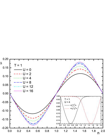
Figure 1: (top) The $\Delta$ parameter as function of the filling $n$ for $T=1$ and $U=0$, $2$, $4$, $8$, $12$ and $16$ (inset: $\xi$ and $\eta$ components for $T=1$ and $U=4$); (bottom) $C^{\alpha}_{11}$ as function of the filling $n$ for $T=2$ and $J=0.05$, the ED data ($4\times 4$) are for $T=0$ and from Ref. Dagotto et al., 1992.

V.1 The $\Delta$ and $p$ parameters

The $\Delta$ and $p$ parameters are computed by solving the system of self-consistent Equations 30 and 33. The behavior of $\Delta$, as function of the filling $n$, is shown in Fig. 1 (top panel). $\Delta$ is defined as the difference between the hopping amplitudes computed between empty and singly occupied sites (i.e., $\langle\xi(i)\xi^{\dagger}(i)\rangle$) and between singly and doubly occupied sites (i.e., $\langle\eta(i)\eta^{\dagger}(i)\rangle$). In this sense, $\Delta$ gives a measure of the electron mobility. The following features have been observed: the hopping amplitude coming from $\xi$ ($\eta$) prevails below (above) half-filling and is always negative [see inset Fig. 1 (top panel)]; the absolute value of $\Delta$ diminishes on increasing the temperature $T$ and on decreasing the Coulomb repulsion $U$. Below half filling, the electrons move preferably among empty and single occupied sites; the same happens to the holes above half filling. This explains the prevalence of one hopping amplitude per each region of filling. In addition, by decreasing the temperature or by increasing the Coulomb repulsion we can effectively reduce the number of doubly occupied sites present in the system and, consequently, favor the mobility of the electrons and increase the absolute value of $\Delta$. These are also the reasons behind the filling dependence: its absolute value first increases with the number of available almost free moving particles ($n\lesssim 0.5$), then decreases when the number of particles is such to allow some double occupancies and to force the reduction of the number of empty sites ($0.5\lesssim n\lesssim 1$) and finally vanishes when, in average, the sites are all singly occupied ($n=1$); the behavior above half filling is equivalent and is related to the holes.

The behavior of $C_{11}^{\alpha}$ within the $t$-$J$ model, as function of the filling $n$, is shown in Fig 1 (bottom panel). Below half filling and for rather high values of the Coulomb repulsion $U$, $\Delta$ and $C_{11}^{\alpha}$ exactly coincide as the $\eta$ component of $\Delta$ completely vanishes. According to this, all the features discussed above for the parameter $\Delta$ are also observed for $C_{11}^{\alpha}$ ($J$ acts like $1/U$). Anyway, we have to report a really small dependence on the exchange interaction $J$ that is fully effective only at $n=1$ where the mobility is already zero as no empty site at all is left. It is worth noting that the exact result for the 2-site system at $T=2$ almost exactly reproduces the Exact Diagonalization (ED)Dagotto et al. (1992) data for a $4\times 4$ cluster at $T=0$. This shows that, by increasing the temperature in a 2-site system it is possible to mime a cluster of bigger size at a lower temperature, at least as regards some of its properties. This can be understood by thinking to the level spacing in the two cases (i.e., bigger the cluster lower the spacing) and to the value of temperature needed to excite those levels. Clearly, not all the properties are in a so strong relation with the relative level positions, but depend on the absolute positions of them. Anyway, this also shows that the relative energy scales/levels are already present in the 2-site system. We have used a value of $J$ twice smaller than the one used within the numerical analysis according to the difference, between the 2-site system and any larger system, regarding the value of the exchange energy $J$ appearing in the derivation of the $t$-$J$ model from the Hubbard oneCastellani et al. (1979). Actually, the derivation is pathological just for the 2-site system and gives a $J$ larger of a factor $2$.

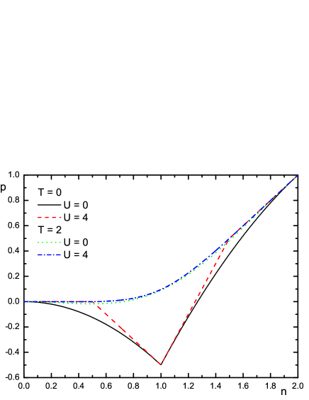
Figure 2: The $p$ parameter as function of the filling $n$ for $T=0$ and $T=2$ at $U=0$ and $U=4$.

As regards the $p$ parameter, in Fig 2 we report its dependence on filling $n$ for two values of the on-site Coulomb repulsion $U=0$ and $U=4$ and for two temperatures $T=0$ and $T=2$. At low temperatures and for $n\lesssim 1.26$, the value of the $p$ parameter is mainly negative according to the antiferromagnetic nature of the spin correlations in the ground state; at higher temperatures the antiferromagnetic spin correlations get weaker and the sign of the parameter changes. The filling $n$, the temperature $T$ and the Coulomb interaction $U$ rule the balance between the spin, the charge and the pair correlations.

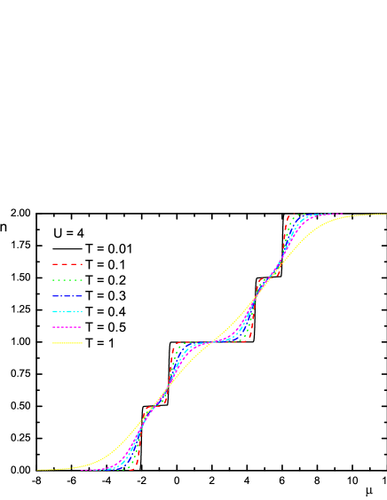
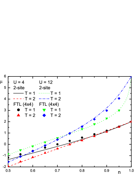
Figure 3: The chemical potential $\mu$ as function of the filling $n$ (top) for $U=4$ and $T=0.01$, $0.1$, $0.2$, $0.3$, $0.4$, $0.5$ and $1$ and (bottom) for $U=4$, $12$ and $T=1$, $2$. The FTL data ($4\times 4$) are taken from Ref. Prelovsek, .

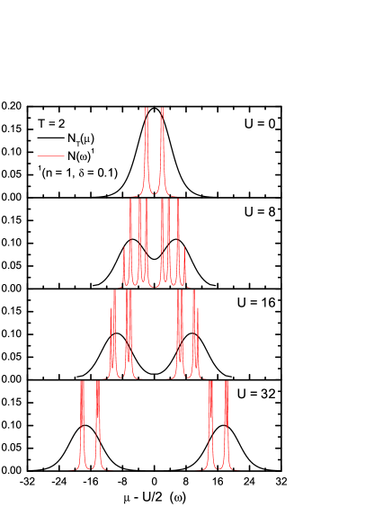
Figure 4: The thermodynamic $N_{T}(\mu)$ and the traditional $N(\omega)$ ($n=1$ and $\delta=0.1$) densities of states as functions of the scaled chemical potential $\mu-U/2$ and the frequency $\omega$, respectively, for $T=2$ and $U=0$, $8$, $16$ and $32$.

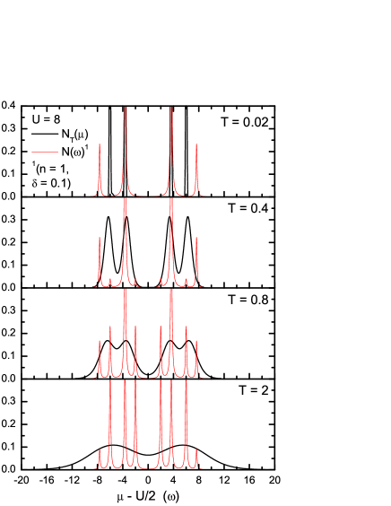
Figure 5: The thermodynamic $N_{T}(\mu)$ and the traditional $N(\omega)$ ($n=1$ and $\delta=0.1$) densities of states as functions of the scaled chemical potential $\mu-U/2$ and the frequency $\omega$, respectively, for $U=8$ and $T=0.02$, $0.4$, $0.8$ and $2$.

V.2 The chemical potential and the density of states

The chemical potential $\mu$ is one of the self-consistent parameters and has been computed by solving the system of self-consistent Equations 30 and 33. As a function of $U$ the chemical potential increases for all studied values of temperature $T$ and filling $n$. In particular, we have the maximum increment for $U\lesssim 20$; for higher values of $U$ the chemical potential saturates. A similar behavior has been reported by numerical data on larger clustersDagotto et al. (1991, 1992); Furukawa and Imada (1992, 1993). In Fig. 3, we show the filling dependence of the chemical potential for some values of the temperature $T$ at $U=4$ (top panel) and for $U=4$, $12$ and $T=1$, $2$ (bottom panel). The Finite Temperature Lanczos (FTL) data ($4\times 4$) are taken from Ref. Prelovsek, . At low temperatures, the chemical potential has a step-like behavior which recalls the discreteness of the energy levels. At higher temperatures, the step-like feature is smeared out due to the thermal hybridization of the energy levels. It is again really noteworthy the agreement between the 2-site results and the numerical data. No temperature adjustment has shown to be necessary in this case as the temperature is already quite high [cfr. Fig. 12 (bottom)]. Generally, the agreement is better for high temperatures and high values of the Coulomb repulsion. Anyway, there is a competition between the temperature smearing effects on the level spacing and the possibility to access the states with energy $J_{U}$ at lower temperatures for higher values of $U$ ($J_{U}\propto 1/U$). Actually, the number of accessible states is comparable for medium temperatures and too large for very high temperatures. This should explain the deviations for $U=4$ and $T=1$, and $U=12$ and $T=2$ at low doping.

By looking at these plots we could be induced to consider the possibility of a metal-insulator transition driven by the Coulomb repulsion $U$ and controlled by the temperature $T$. Obviously, no such transition is possible in a finite system that is always in a metal paramagnetic state for any finite or zero value of the Coulomb repulsion $U$; we will show, in Sec. V.8, that the Drude weight is always finite. Such tricky behavior of the chemical potential can be understood by thinking at the nature of the grand canonical ensemble we are using for our thermal averages. As we are very far from the thermodynamic limit, there is no equivalence at all among the micro-, the grand- and the canonical ensembles. In particular, whenever we speak about temperature and chemical potential in a finite system we have just to think in terms of mixtures of quantum mechanical states with different energies and numbers of particles. To get a deeper comprehension of this issue we can define a thermodynamic density of states $N_{T}(\mu)$ through the following equation

$$n=\int_{-\infty}^{\mu}\!d\omega N_{T}(\omega)$$ (174)

which is a generalization to finite temperatures of the identical relation existing, at zero temperature, between the filling $n$ and the usual density of states $N(\omega)$. In general, the two densities of states coincide only at zero temperature and for systems, like the non-interacting ones, whose density of states is independent on the chemical potential $\mu$. From the definition (174), we can simply compute the thermodynamic density of states $N_{T}(\mu)$ by differentiating the filling $n$ with respect to the chemical potential $\mu$ [$N_{T}(\mu)=\emph{d}n/\emph{d}\mu$]. It is worth mentioning that the thermodynamic density of states $N_{T}(\mu)$, apart from a factor $\frac{1}{n^{2}}$, is simply the compressibility of the system. A vanishing value of this quantity denotes the impossibility for the system to accept more particles and, obviously, the presence of a gap. The thermodynamic density of states $N_{T}(\mu)$ enormously facilitates the comprehension of the chemical potential features that are singled out by the differentiation procedure. The usual density of states $N(\omega)$ is computed as follows

$$N(\omega)=\frac{1}{2}\sum_{n=1}^{4}\sum_{k}\delta\!\left[\omega-E_{n}(k)\right]\sigma_{cc}^{(n)}(k)$$ (175)

Both densities of states are reported in Figs. 4 and 5 as function of the chemical potential ($\mu$) and the frequency ($\omega$), respectively. We have computed $N(\omega)$ by substituting, for obvious graphical reasons, the Dirac deltas ($\delta(\omega)$) with Lorentzian functions ($\frac{1}{\pi}\frac{\delta}{\omega^{2}+\delta^{2}}$) with $\delta=0.1$. In reporting the thermodynamic density of states $N_{T}(\mu)$ we have scaled the chemical potential $\mu$ by its value at half filling ($U/2$) as we want to make the comparison for this particular value of $n$. While $N(\omega)$ always presents a gap at $\omega=0$ (the overlapping tails are due to the finite $\delta$ and the non-zero kinetic energy ensures a metallic behavior), $N_{T}(\mu)$ shows a gap only above a certain value of the Coulomb repulsion for a fixed $T$ (see Fig. 4) and below a certain temperature for a fixed $U$ (see Fig. 5). We want to emphasize that, at high temperature, $N_{T}(\mu)$ is capable to mime the behavior expected for the lattice system. In particular, $N_{T}(\mu)$ presents two well defined structures (i.e., the two Hubbard subbands) that continuously separate on increasing $U$ (see Fig. 4). This behavior is the one expected, after many analytical and numerical results, for the bulk at dimension greater than one and it is a realization of the metal-insulator transition according to the Mott-Hubbard mechanism. It is worth noting that, for this small system, the critical Coulomb repulsion, at which the gap appears, is a function of the temperature $T$.

The density of states $N(\omega)$ is also reported in order to give an idea of the positions of the poles and of the relative intensity of the spectral weights, although we had to cut the highest peaks in drawing the pictures. We can observe two relevant features. In the non-interacting case ($U=0$) only two poles/peaks are present; those coming from the band $E_{1}(k)$ and separated by the bandwidth $W=4t$. On increasing the Coulomb potential $U$ the three scales of energy present in the system clearly manifest themselves: the exchange interaction $J_{U}$, the bandwidth $W$ and the Coulomb repulsion $U$. The eight poles group in two main structures separated by $U$. Within any structure the four poles are separated according to the combination of $\pm 2t$ (bandwidth separation) and the presence or absence of the exchange interaction $J_{U}$. The bandwidth $W$ is obviously $U$ independent and generates a rigid two peak structure for any band $E_{n}(k)$. On the contrary, the exchange energy $J_{U}$ decreases on increasing $U$ with a consequent reduction of the resolution of the peaks within the Hubbard subbands. The other relevant feature is the redistribution of the total spectral weight on increasing the temperature. At low temperatures the poles/peaks that do not contain the exchange interaction $J_{U}$ have negligible spectral weights; the 2-site singlet is the ground state at half-filling. On increasing temperature the total spectral weight redistributes and the other poles get more and more spectral weight due to the thermal hybridization of the energy levels.

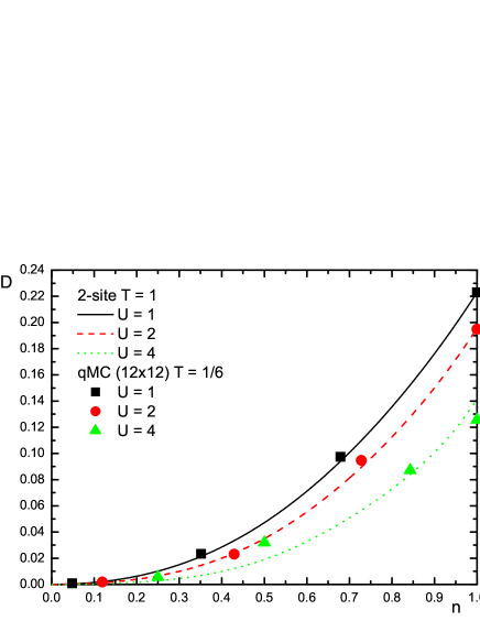
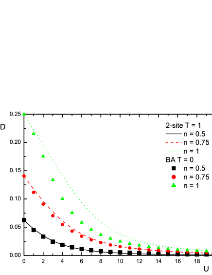
Figure 6: The double occupancy $D$: (top) as function of the filling $n$ for $U=1$, $2$ and $4$ at $T=1$, the qMC data ($12\times 12$) are for $T=1/6$ and from Ref. Moreo et al., 1990; (bottom) as function of the Coulomb repulsion $U$ for $n=0.5$, $0.75$ and $1$ at $T=1$, the BA data are for $T=0$.

V.3 The double occupancy $D$

In the non-interacting case ($U=0$) we have $D=n^{2}/4$. At zero temperature, the double occupancy $D$ vanishes for $n\leq 0.5$; below this value of filling we have, in average, less than one electron in the system and only for a finite temperature we can get some contributions by states with a finite double occupancy. At half filling we have the following exact formula for the double occupancy at zero temperature

$$D=\frac{2J_{U}}{U+8J_{U}}$$ (176)

The filling dependence of the double occupancy $D$ (top panel) is reported in Fig. 6 for several values of the Coulomb repulsion $U$ at temperature $T=2$. There are also reported some quantum Monte Carlo (qMC) dataMoreo et al. (1990) for a bigger cluster ($12\times 12$). As in the case of $C_{11}^{\alpha}$ within the $t$-$J$ model, we note that the exact results for the 2-site system at temperature $T=1$ very well reproduce the quantum Monte Carlo (qMC) data for the bigger cluster at $T=1/6$. The same explanation obviously holds. A comparison with the exact results from Bethe Ansatz (BA) are also reported in Fig. 6 (bottom panel). Also in this case the 2-site system manage to reproduce the bigger cluster data (actually, the Bethe Ansatz (BA) system is the 1D bulk) by increasing the temperature. The discrepancy at half filling can be understood as a consequence of the difference in the definition of the exchange energy $J$ discussed in the Section regarding the internal energy. Obviously, the discrepancy is larger where the exchange interaction is mainly effective (i.e., at half filling and for intermediate-strong values of the Coulomb interaction).

V.4 Thermodynamics

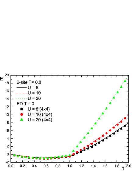
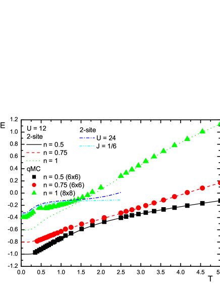
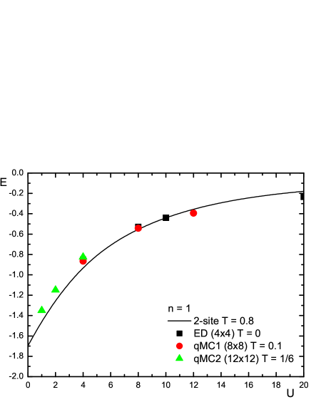
Figure 7: The energy $E$: (top) as function of the filling $n$ for $T=0.8$ and $U=8$, $10$ and $20$, the ED data ($4\times 4$) are for $T=0$ and from Ref. Dagotto et al., 1992; (middle) as function of the temperature $T$ for $U=12$ and $n=0.5$, $0.75$ and $1$ [$U=24$ and $J=1/6$ ($t$-$J$ mode) data are also reported], the qMC data ($6\times 6$ and $8\times 8$) are from Ref. Duffy and Moreo, 1997; (bottom) as function of the Coulomb repulsion $U$ for $n=1$ and $T=0.8$, the ED data ($4\times 4$) are for $T=0$ and from Ref. Dagotto et al., 1992, the qMC1 data ($8\times 8$) are for $T=0.1$ and from Ref. Duffy and Moreo, 1997, the qMC2 data ($12\times 12$) are for $T=1/6$ and from Ref. Moreo et al., 1990.

V.4.1 The energy $E$, the specific heat $C$ and the entropy $S$

The energy per site $E$ is computed as thermal average of the Hamiltonian divided by the number of sites. Its filling dependence is reported in Fig. 7 (top panel) together with some Exact Diagonalization (ED) data for bigger clustersDagotto et al. (1992). As expected, the energy $E$ increases as the Coulomb repulsion $U$ increases. For $n<1$ and high values of the Coulomb repulsion the kinetic term prevails on the Coulomb one. The opposite behavior is observed for $n>1$. The behavior as a function of the temperature $T$ and Coulomb repulsion $U$ are reported in Fig. 7 (middle and bottom panels, respectively) together with some data coming from numerical analysis for bigger clustersMoreo et al. (1990); Dagotto et al. (1992); Duffy and Moreo (1997). By using a higher temperature for the 2-site data is again possible to get an extremely good agreement with the numerical results [see Fig. 7 (top and bottom panels)]. In the case of the temperature behavior instead, the agreement is obtained without tuning any parameter [see Fig. 7 (middle panel)].

The discrepancy at half filling and low temperatures [see Fig. 7 (middle panel)] is a consequence of the different value of the exchange energy $J$ appearing in the derivation of the 2-site $t$-$J$ model from the Hubbard one (see detailed discussion about the behavior of $C^{\alpha}_{11}$ reported in Fig. 3 (bottom panel), Sec. V.1). According to this, at half-filling and low temperatures we have also reported the 2-site results for $U=24$ and $J=1/6$ ($t$-$J$ model) and obtained the expected agreement. The reason why no effect is evident for lower fillings and high temperatures is that the exchange interaction is really effective only at half-filling (in average one spin per site is necessary) and low temperatures (the fluctuations should be small).

In Fig. 8 we show the temperature dependence of the specific heat $C=dE/dT$ for several values of $U$ at $n=0.75$ and $n=1$. For $n\neq 1$ we have three peaks at temperatures of the order half ($0.3\div 0.6$) the scales of energies $J_{U}$, $t$ and $U$. This is in agreement with the behavior of a pure two- or three- gap system in the canonical ensemble. The effect of increasing the Coulomb repulsion $U$ is a better resolution of the three peaks. In fact, the first one moves towards lower temperatures, the second one is stable and the third moves to higher temperatures; this is in perfect agreement with their origins: $1/U$, $t$ and $U$, respectively. At half filling nothing changes except for the absence of the middle peak: the single occupied states do not contribute. It is worth mentioning that the kinetic peak appears as the energy levels corresponding to different values of the momentum are here discrete as in any finite system. No such a peak is present in infinite systems where the kinetic energy just spreads over a band the energy levels coming from the interactions.

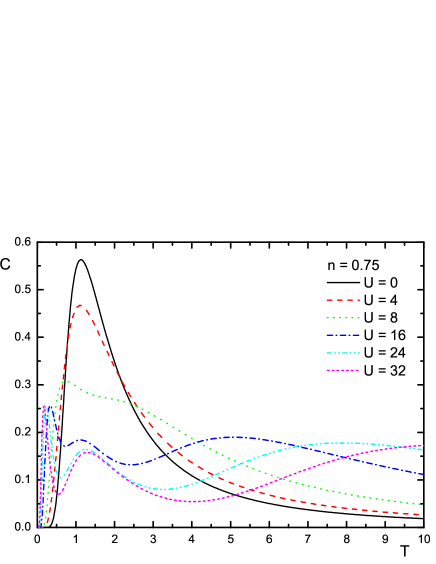
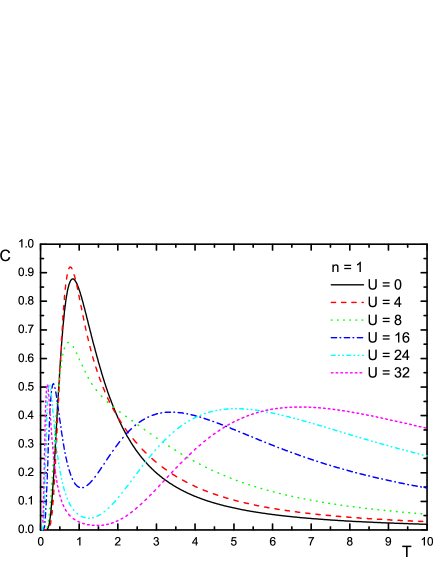
Figure 8: The specific heat $C$: as function of the temperature $T$ for $n=0.75$ (top) [$n=1$ (bottom)] and $U=0$, $4$, $8$, $16$, $24$ and $32$.

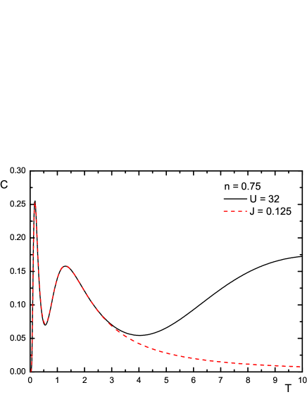
Figure 9: The specific heat $C$ as function of the temperature $T$ for $n=0.75$ and $U=32$ and $J=0.125$.

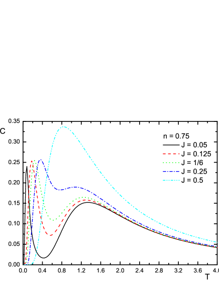
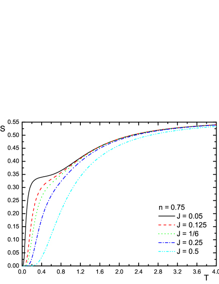
Figure 10: (top) The specific heat $C$ as function of the temperature $T$ for $n=0.75$ and $J=0.0.5$ , $0.125$, $1/6$, $0.25$ and $0.5$; (bottom) The entropy $S$ as function of the temperature $T$ for $n=0.75$ and $J=0.0.5$ , $0.125$, $1/6$, $0.25$ and $0.5$.

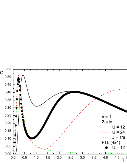
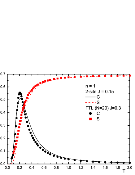
Figure 11: (top) The specific heat $C$ as a function of the temperature $T$ for $U=12$ at $n=1$. The $U=24$ and $J=1/6$ ($t$-$J$ mode) data are also reported. The FTL data ($4\times 4$) are taken from Ref. Bonca and Prelovsek, 2003. (bottom) The specific heat $C$ and the entropy $S$ as functions of the temperature $T$ for $J=0.15$ at $n=1$. The FTL data ($N=20$) are from Ref. Jaklic and Prelovsek, 2000.

The specific heat $C$ is a really valuable property to quantify how good is the $t$-$J$ model to describe the low energy dynamics of the Hubbard model. We have studied $C$ as a function of both $4t^{2}/U$ and $J$ in the Hubbard and $t$-$J$ model, respectively. We need a Coulomb repulsion $U\geq 24t$ ($4t^{2}/U\leq\frac{1}{6}t$) to have the possibility of a faithful mapping at low temperatures; only for such values of $U$ we manage to sufficiently resolve the three scales of energy in the Hubbard model. For instance, at $U=32\Leftrightarrow J=0.125$ the mapping can be absolutely trusted as shown in Fig. 9 where we report the specific heat for $n=0.75$. As regards the exchange and kinetic peaks the agreement is perfect; obviously the $t$-$J$ model cannot reproduce the Coulomb peak, which is extraneous to its dynamics. The absence of the kinetic peak at half filling is also perfectly reproduced (see Fig. 11).

In Fig. 10 (top panel) we report the behavior, in the $t$-$J$ model, of the specific heat as function of the temperature $T$ for different values of the exchange constant $J$. It is worth mentioning that in the $t$-$J$ model the two peaks in the specific heat (i.e., the exchange and kinetic peaks) can be easily studied separately as they just come from the corresponding terms of the Hamiltonian. This simple analysis cannot be performed in the Hubbard model where the exchange peak gets contribution from both terms of the Hamiltonian.

In Fig. 10 (bottom panel) we report the entropy $S$ of $t$-$J$ model computed by means of the usual thermodynamic relations from the specific heat $C$

$$S(T)=\int_{0}^{T}\frac{d\tilde{T}}{\tilde{T}}C(\tilde{T})$$ (177)

We can easily put in correspondence the peaks of the specific heat [see Fig. 10 (middle panel)] and the change in the slope of the entropy. Again, a lowering of the exchange energy $J$ helps resolving the scales of energy and makes much more visible the difference in the slopes.

In Fig. 11, it is reported the specific heat as a function of the temperature for the Hubbard model (top panel) and the $t$-$J$ model (bottom panel). For this latter, it has been also reported the entropy. The Finite Temperature Lanczos (FTL) data for the Hubbard model ($4\times 4$) and for the $t$-$J$ model ($N=20$) are taken from Ref. Bonca and Prelovsek, 2003 and Ref. Jaklic and Prelovsek, 2000, respectively. The agreement is absolutely noteworthy on the whole temperature range. Again, the discrepancy at low temperatures in the Hubbard model case is a consequence of the difference regarding the value of the exchange energy $J$. According to this, we have also reported the 2-site results for $U=24$ and $J=1/6$ ($t$-$J$ model) and obtained the expected agreement. In the $t$-$J$ model case, we have used a value of $J$ twice smaller than the one used within the numerical analysis according to the boundary conditions we applied to the 2-site system. These results show, once more, that the correct and necessary scales of energies are already present in the 2-site system.

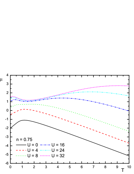
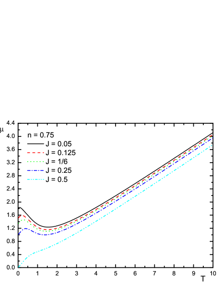
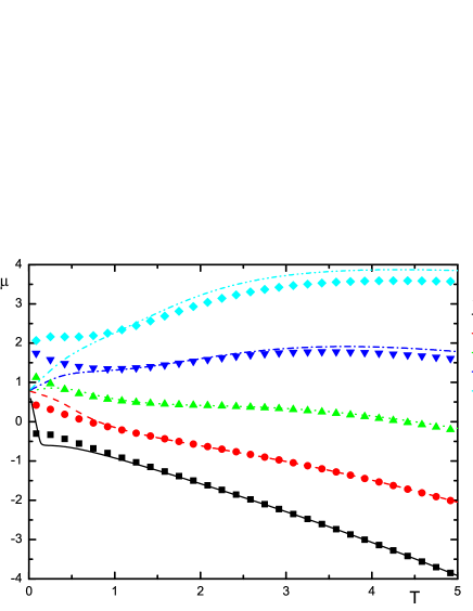
Figure 12: The chemical potential $\mu$: (top) as function of the temperature $T$ for $n=0.75$ and $U=0$, $4$, $8$, $16$, $24$ and $32$; (middle) as function of the temperature $T$ for $n=0.75$ and $J=0.05$ , $0.125$, $1/6$, $0.25$ and $0.5$; (bottom) as function of the temperature $T$ for $U=12$ and $n=0.5$, $0.6$, $0.7$, $0.8$ and $0.9$. The FTL data ($4\times 4$) are from Ref. Prelovsek, .

V.4.2 The temperature dependence of
the chemical potential $\mu$ and the double occupancy $D$

The temperature dependence of the chemical potential $\mu$ is given in Fig. 12 (top panel). $\mu$ has only one maximum for $U\lesssim 8$ and two maxima and a minimum for higher values of $U$. In the $t$-$J$ model, the chemical potential $\mu$ shows a behavior at low temperatures in agreement with the one found for the Hubbard model (i.e., $\lim_{U\gg t}J_{U}=J$). On the contrary, for high temperatures the divergence is upward instead of downward [see Fig. 12 (bottom panel)].

The temperature dependence of the chemical potential can be explained as follows. In the Hubbard model and at zero temperature, there exists a critical value of the Coulomb interaction, function of the filling, above which the potential energy becomes larger, in absolute value, than the kinetic one. This critical value is a decreasing function of the filling: lower is the doping higher the double occupancy, bigger the potential energy and smaller, in absolute value, the kinetic energy. Then, by increasing the filling we increase the energy and the chemical potential increases. At higher and higher temperatures, the system behaves like a free system at zero temperature and has a decreasing chemical potential. In particular, for a diverging temperature we have a negatively diverging chemical potential (i.e., $\mu=dE/dn-TdS/dn$) as the entropy is an increasing function of the filling at very high temperatures (i.e., in the almost free case) and $n<1$. For intermediate temperatures, the chemical potential has maxima and minima in coincidence with the peaks in the specific heat. Any peak in the specific heat marks the temperature at which the system gets the freedom to occupy a new state. The spin (i.e., $T\sim J_{U}$) and the charge (i.e., $T\sim U$) peaks reflect in two maxima as they signal the availability of triplet states and of doubly occupied states, respectively. Both states has zero kinetic energy. On the contrary, the kinetic (i.e., $T\sim t$) peak signals the availability of further singly occupied states which maximize the absolute value of the kinetic energy. This reasoning strongly relies on the region of filling the figure refers to (i.e., $n\approx 0.75$). For other doping regions the situation can be quite different owing to the behavior in filling of the double occupancy, the entropy and the positions and existence of the peaks in the specific heat. These considerations can also explain the quite different behavior we have in the $t$-$J$ model. At $n=0.75$ the $t$-$J$ model is approaching the full-filled system (i.e., $n=1$), on the contrary the Hubbard model is approaching the half-filled system. At zero temperature for $n>0.5$, increasing the filling we lowers, in absolute value, the kinetic energy as the single electron states, which are the only ones with a finite kinetic energy, are replaced by the singlet and triplet states: the chemical potential is positive. Anyway, the exchange energy can effectively lower its value on increasing $J$. At very high temperatures (i.e., in the almost free case), the entropy is now a decreasing function of the filling and leads to the positive divergence. At intermediate temperatures, the reasoning is identical to the one given for the Hubbard model except for the obvious absence of the charge peak in the $t$-$J$ model.

In Fig. 12 (bottom), it is reported the chemical potential as function of the temperature $T$ for $U=12$ and $n=0.5$, $0.6$, $0.7$, $0.8$ and $0.9$. The FTL data ($4\times 4$) are from Ref. Prelovsek, . The agreement is really excellent except at low temperatures and for the higher values of the filling ($n=0.8$ and $n=0.9$). At low temperatures, owing to the finite level spacing the chemical potential has a step behavior and, in particular, between $n=0.5$ and $n=0.9$ has practically no variation (cfr. Fig 3). At the higher values of the filling ($n=0.8$ and $n=0.9$), the number of 2-site states excited at high temperatures is larger than those needed to mime the cluster.

The temperature dependence of the double occupancy $D$ at half filling shows a minimum at around $T\approx 1$ before saturating at the non-interacting value $n^{2}/4$ for very high temperaturesGeorges and Krauth (1993); Schulte and Böhm (1996). This minimum coincides with the kinetic peak in the specific heat. As already discussed for the chemical potential, this peak marks the freedom for the system to occupy further singly occupied states which have, obviously, zero double occupancy and, therefore, lower its total value.

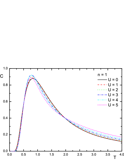
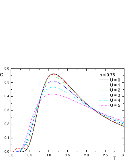
Figure 13: The specific heat $C$ as function of the temperature $T$ for $n=1$ (left panel) [$n=0.75$ (right panel)] and $U=0$, $1$, $2$, $3$, $4$ and $5$.

V.4.3 The crossing points

In Fig. 13 we report the temperature dependence of the specific heat for $U\leq 5t$ at half filling (top panel) and $n=0.75$ (bottom panel). For these low values of the Coulomb repulsion we identify three crossing points/regions where the specific heat is almost independent from the value of the Coulomb repulsion $U$Vollhardt (1997); Chandra et al. (1999); Mancini et al. (1999). To compute the positions and heights of the crossing points we have expanded the specific heat $C$ as function of the Coulomb repulsion $U$. We have got

$$C(T,U,n)=C_{0}(T,n)+C_{2}(T,n)U^{2}+O\left(U^{4}\right)$$ (178a)

$$C_{0}(T,n=1)=2\beta^{2}t^{2}\left[1-\tanh^{2}\left(\beta t\right)\right]$$ (178b)

$$C_{2}(T,n=1)=\frac{\mathrm{e}^{2\beta t}}{8T^{4}\left(1+\mathrm{e}^{2\beta t}\right)^{6}}\left[48t^{2}\mathrm{e}^{2\beta t}\left(1-3\mathrm{e}^{2\beta t}+\mathrm{e}^{4\beta t}\right)+2tT\left(1+20\mathrm{e}^{2\beta t}-20\mathrm{e}^{6\beta t}-\mathrm{e}^{8\beta t}\right)+2T^{2}\left(1+\mathrm{e}^{2\beta t}\right)^{4}\right]$$ (179)

The temperatures $T^{*}(n)$ at which the crossing point can be observed are determined by the equation $C_{2}(T,n)=0$. At half filling and at $n=0.75$, this equation gives the following results:

$$T^{*}_{1}(n=1)\cong 0.499\quad\Rightarrow\quad C_{0}\cong 0.563$$ (180a)

$$T^{*}_{2}(n=1)\cong 0.997\quad\Rightarrow\quad C_{0}\cong 0.841$$ (180b)

$$T^{*}_{3}(n=1)\cong 2.058\quad\Rightarrow\quad C_{0}\cong 0.376$$ (180c)

$$T^{*}_{1}(n=0.75)\cong 0.951\quad\Rightarrow\quad C_{0}\cong 0.523$$ (181a)

$$T^{*}_{2}(n=0.75)\cong 2.024\quad\Rightarrow\quad C_{0}\cong 0.342$$ (181b)

Vollhardt found an approximate formula for $C_{0}$ and $T^{*}$, as function of the dimensionality of the system, for the higher temperature crossing point at half fillingChandra et al. (1999). The values that this formula gives for $d=1$, the dimensionality of the 2-site system within periodic boundary conditions, are close, as regards $C_{0}$, to the exact ones of Eq. (180c).

It is worth noting that higher is the temperature narrower is the crossing region; ranging from quite wide regions for the two lower temperatures to a very sharp point for the higher temperature. Also the chemical potential (Fig. 3 (top panel) at $n\approx 0.275,0.75,1.25,1.725$) and the double occupancy show quite clear crossing points in (no dependence on) temperature.

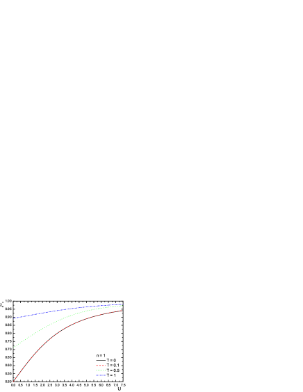
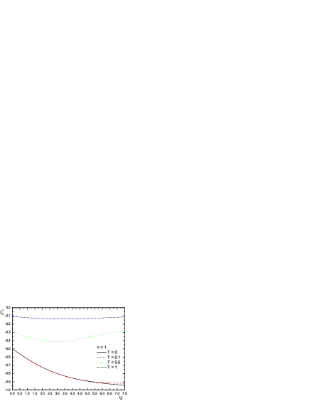
Figure 14: The charge $\chi^{\alpha}_{c}$ (top) and spin $\chi^{\alpha}_{s}$ (bottom) correlation functions as functions of $U$ at $n=1$ and for $T=0$, $0.1$, $0.5$ and $1$.

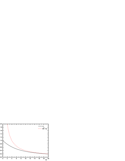
Figure 15: Comparison between $J_{U}$ and its limiting value $4t^{2}/U$ as functions of $U$.

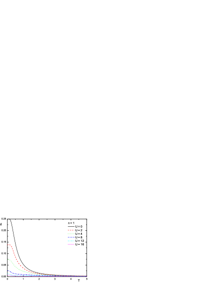
Figure 16: The pair correlation function $d$ as function of $T$ at $n=1$ and for $U=0$, $2$, $4$, $8$, $12$ and $16$.

V.5 Charge, spin and pair correlations

The charge (i.e., $\chi_{c}^{\alpha}$), spin (i.e., $\chi_{s}^{\alpha}$) and pair (i.e., $d$) correlation functions contain information regarding the spatial distributions of the corresponding quantities. Obviously, we can only consider the quantum fluctuations in the paramagnetic state, which is the only admissible equilibrium state on a finite cluster.

The charge correlation function $\chi_{c}^{\alpha}$ is shown in Fig. 14 (top) as function of the interaction $U$ for different values of the temperature $T$ and $n=1$. In the non-interacting case ($U=0$) and at zero temperature we have

$$\chi_{c}^{\alpha}-n^{2}=\left\{\begin{tabular}[]{lll}$-\frac{1}{2}n^{2}$&if&$n\leq 1$\\ $-\frac{1}{2}\left(2-n\right)^{2}$&if&$n\geq 1$\end{tabular}\right.$$ (182)

as only the singlet states with one electron ($n\leq 1$) [one hole ($n\geq 1$)] per site contribute. In fact, these are the states which lower the most the internal energy as they maximize the absolute value of the kinetic one. In the strongly interacting limit ($U\rightarrow\infty$) and at zero temperature we have

$$\chi_{c}^{\alpha}-n^{2}=\left\{\begin{tabular}[]{lll}$-n^{2}$&if&$n\leq 0.5$\\ $-\left(1-n\right)^{2}$&if&$0.5\leq n\leq 1.5$\\ $-\left(2-n\right)^{2}$&if&$n\geq 1.5$\end{tabular}\right.$$ (183)

as only the states with a single electron ($n\leq 0.5$) [a single hole ($n\geq 1.5$)] or only with one electron per site ($0.5\leq n\leq 1$) [one hole per site ($1\leq n\leq 1.5$)] contribute. In fact, no double occupancy is allowed and there is no gain in the kinetic energy if the singlet states are used as $J_{U}\rightarrow 0$. At intermediate values of the coupling $U$ the double occupied states play a relevant role and we found results between the limiting cases reported above: on increasing the coupling $U$ the double occupancy diminishes and consequently the states with one electron per site increase their contribution and the value of $\chi_{c}^{\alpha}$ (see Fig. 14 (top)). On increasing the temperature $T$, more and more states become available and the correlation tends to its reducible part, $n^{2}$.

The spin correlation function $\chi_{s}^{\alpha}$ is reported in Fig. 14 (bottom) for the same parameters chosen for $\chi_{c}^{\alpha}$. In the non-interacting case ($U=0$), we have $\chi_{s}^{\alpha}=\chi_{c}^{\alpha}$: in absence of interaction the charge and spin behave coherently. On increasing the interaction potential $U$ the singlet states are favored and the spin correlations get enhanced ($J_{U}$ gets closer and closer to $4t^{2}/U$ which is the scale of energy of the spin excitations, see Fig. 15). Then, further increasing $U$ the value of $J_{U}$ tends to zero and the spin correlations get suppressed except at zero temperature [see Fig. 14 (bottom)]. A rapid suppression of the spin fluctuations can be caused also by the increment of the temperature.

The pair correlation function $d$ is reported in Fig. 16 as function of the temperature $T$ at $n=1$ and for $U=0$, $2$, $4$, $8$, $12$ and $16$. Obviously, $d$ decreases on increasing the Coulomb interaction $U$ and is maximum at half-filling where the singlet state is the favorite one. On increasing the temperature $T$ (see Fig. 16), more and more states become available and the pair correlation function $d$ tends to zero.

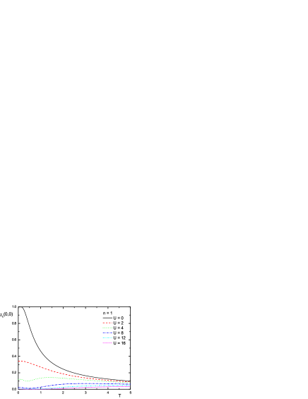
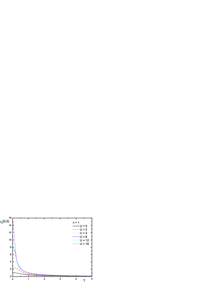
Figure 17: The charge $\chi_{c}(0,0)$ (top) and spin $\chi_{s}(0,0)$ (bottom) susceptibilities as functions of $T$ at $n=1$ for $U=0$, $2$, $4$, $8$, $12$ and $16$.

V.6 Charge and spin susceptibilities

The charge and spin susceptibilities $\chi_{\mu}(k,\omega)$ are given by

$$\chi_{\mu}(k,\omega)=-\mathcal{F}\left\langle\mathcal{R}[n_{\mu}(i)n_{\mu}(j)]\right\rangle$$ (184)

where no summation is implied by repeated indices. By means of the expression of the causal Green’s function given in Sec. IV.2.1 is immediate to compute the following static susceptibilities through the spectral theorem

$$t\chi_{c}(k,0) =-C_{cc}^{\alpha}-\frac{U}{2t}d$$ (185)

$$t\chi_{s}(k,0) =-C_{cc}^{\alpha}-\frac{1}{12}\frac{U}{t}\chi_{s}^{\alpha}$$ (186)

where $d$ and $\chi_{s}^{\alpha}$ are the first-neighbor pair and spin correlation functions, respectively.

In Fig. 17, the charge $\chi_{c}(k,0)$ and spin $\chi_{s}(k,0)$ susceptibilities are reported as function of the temperature $T$ for different values of the Coulomb repulsion $U$ and $n=1$. As it results clear by Eqs. 185, the two susceptibilities result identical in the non-interacting case $U=0$: once more charge and spin behave coherently in absence of interaction. On increasing the Coulomb repulsion, the two susceptibilities behave in opposite manners: the charge susceptibility is strongly suppressed, in particular at half-filling where a charge gap develops in the strongly interacting limit ($U\rightarrow\infty$); the spin susceptibility is greatly enhanced, in particular at half-filling where the singlet state is the favorite one. The behavior of the two susceptibilities as functions of the temperature deserve special attention as it is directly connected with the formation of a gap in the corresponding channel. The spin susceptibility shows the typical paramagnetic behavior: plateau at low temperatures and Curie tail at high temperatures. The charge susceptibility instead shows the presence of a gap in the strongly interacting limit ($U\rightarrow\infty$). The small upturn at low temperatures and medium-high values of the Coulomb repulsion $U$ is due to the finite level-spacing of the system. In particular, it arises from the intra-subband gaps characteristic of the scale of energy $J_{U}$.

In the $t$-$J$ model, we simply have

$$t\chi_{c}\left(k,0\right) =-C_{11}^{\alpha}$$ (187)

$$t\chi_{s}\left(k,0\right) =-C_{11}^{\alpha}-\frac{1}{3}\frac{t}{J}\chi_{s}^{\alpha}$$ (188)

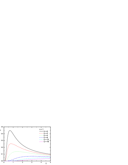
Figure 18: The compressibility $\kappa$ as a function of $T$ at $n=1$ for $U=0$, $2$, $4$, $8$, $12$ and $16$.

V.7 Thermal compressibility

The thermal compressibility is defined as

$$\kappa=\frac{1}{n^{2}}\frac{\partial n}{\partial\mu}$$ (189)

By using some general quantum statistical relations, which can be established between the particle density $n$ and the chemical potential $\mu$ Feng and Mancini (2001), we can express the thermal compressibility in terms of the density-density correlation function

$$\kappa=\frac{1}{Tn^{2}}\left[\left(n+2D-n^{2}\right)+\left(\chi_{c}^{\alpha}-n^{2}\right)\right]$$ (190)

In Fig. 18, the thermal compressibility $\kappa$ is reported as function of the temperature $T$ for different values of the Coulomb repulsion $U$ and $n=1$. The system is completely incompressible $\kappa=0$ when no more particles are allowed to enter the system: the chemical potential, which is a measure of the energy necessary to insert a new particle in the system, diverges. Obviously, the system is extremely eager to accept particles at very low fillings, in order to increase in absolute value the kinetic energy and lower the total one, and absolutely incompressible at $n=2$, when all the quantum states are filled. At zero temperature, the Coulomb repulsion makes incompressible also the states with commensurate fractional fillings $n=0.5$ and $n=1.5$. At half-filling, on increasing the Coulomb repulsion, the compressibility is rapidly suppressed according to the very high price in energy that should be paid to add one particle to the singlet state which is the one favored by the Coulomb repulsion. The most relevant feature for this property is the presence of a well-defined peak when it is plotted versus temperature. A finite, but low in comparison with the actual value of the Coulomb repulsion, temperature permits to overcome the suppression related to the formation of a charge gap. A further increment of the temperature makes available more and more states and the system is driven back to be incompressible.

It is possible to write the compressibility for the Hubbard and $t$-$J$ models in an identical way

$$\kappa=\frac{2}{Tn^{2}}\left(\Gamma_{11c}-n^{2}\right)$$ (191)

where $\Gamma_{11c}$ is the zero frequency function in the charge channel and its ergodic value is exactly $n^{2}$. According to this, the compressibility is a direct measure of the ergodicity of the charge dynamics.

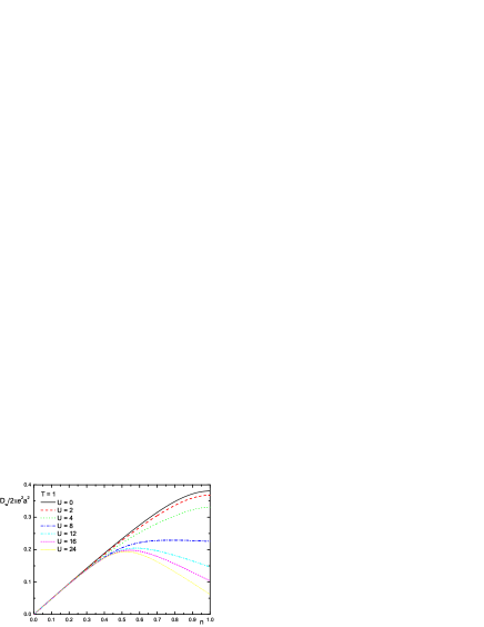
Figure 19: The Drude weight $D_{w}$ as a function of $n$ for $T=1$ and $U=0$, $2$, $4$, $8$, $12$, $16$ and $24$.

V.8 Optical conductivity

In the framework of the linear response and by using the Ward-Takahashi identitiesMancini:98a, which relate the current-current propagator to the charge-charge one by exploiting the charge conservation, the optical conductivity is given by

$$\sigma_{1}(\omega)=D_{w}\delta(\omega)$$ (192)

with the Drude weight $D_{w}$ given by

$$D_{w}=-4\pi\mathrm{e}^{2}a^{2}tC_{cc}^{\alpha}$$ (193)

For the 2-site system, the incoherent part of optical conductivity is zero as no contribution comes from the imaginary part of retarded current-current propagator.

In Fig. 19, the Drude weight $D_{w}$, normalized by $2\pi\mathrm{e}^{2}a^{2}$, is reported as function of the filling $n$ for different values of the Coulomb repulsion $U$ and $T=1$. At half-filling, the Coulomb repulsion tends to suppress the Drude weight and drives the system to be insulating. However, the Drude weight vanishes only in the limit $U$ infinite. Higher the temperature more states with no contribution to the kinetic energy result available and lower is the Drude weight.

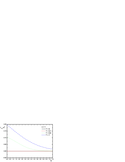
Figure 20: The charge zero frequency constant $\Gamma_{11c}$ diminished of $n^{2}$: (top) as function of $n$ for $T=0.1$ and $U=0$, $2$, $4$, $8$, $12$ and $16$; (bottom) as function of $U$ at $n=1$ and for $T=0$, $0.1$, $0.5$ and $1$.

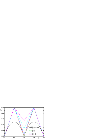
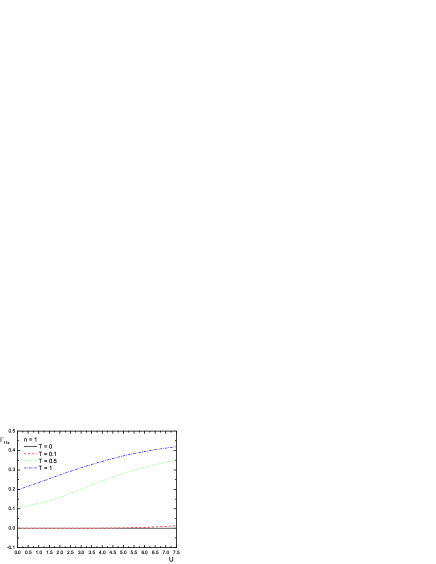
Figure 21: The spin zero frequency constant $\Gamma_{11s}$: (top) as function of $n$ for $T=0.1$ and $U=0$, $2$, $4$, $8$, $12$ and $16$; (bottom) as function of $U$ at $n=1$ and for $T=0$, $0.1$, $0.5$ and $1$.

VI Ergodicity

One of the main issues on which this manuscript wishes to draw attention is the non-ergodicity of the charge and spin dynamics in the two-site Hubbard model. The non-ergodic dynamics in this system is due to the finite number of degenerate states available to the system when dealing with finite temperatures and/or incommensurate fillings and/or no interaction (cfr. Table 1 and Eq. 205). The finite level spacing confines the system to degenerate or non-degenerate states, according to the filling and interaction strength, making the dynamic ergodic or non-ergodic according to the degree of degeneracy of the ground state. The temperature then opens up the possibility for quite complicate mixtures, only possible according to our choice to work in the grand-canonical ensemble in order to get results comparable with larger systems for which the level spacing is thinner. The coupling to an heat and a particle reservoirs have given us the possibility to simulate a continuous tuning of the filling and temperature on a finite system (with a finite degree of freedom) as it is possible only in a bulk system with infinite degrees of freedom.

The zero-frequency constants for charge $\Gamma_{11c}$ and spin $\Gamma_{11s}$ channels have been plotted as functions of the filling $n$ for different values of the Coulomb repulsion $U$ and $T=0.1$ and as functions of the interaction $U$ for different values of temperature $T$ and $n=1$ in Figs. 20 and 21. Their ergodic values are $n^{2}$ and $0$, respectively. $\Gamma_{11c}$ assumes its ergodic value only at zero temperature and commensurate fillings; in particular, only at integer commensurate fillings for any interaction strength and also at fractional ones for a finite interaction strength. On the other hand, $\Gamma_{11s}$ assumes its ergodic value only at zero temperature and integer commensurate fillings for any interaction strength. At half-filling, while the charge dynamics is constrained to be ergodic in the strongly interacting limit ($U\rightarrow\infty$) by the formation of a charge gap, the spin dynamics gets more and more non-ergodic as larger the interaction strength is. The states that are left available in this condition have a quite different behavior once probed with respect to the charge or spin response.

VII Conclusions

We have studied the 2-site Hubbard and $t$-$J$ models by means of the Green’s function and equations of motion formalism. The main results can be so summarized:

• We have got a complete basis of eigenoperators for the fermionic and bosonic sectors which could be used to get a controlled approximation in the study of the lattice case by means of any approximation that strongly relies on the choice of the basic field.

• We have identified the eigenoperator responsible for the appearance of the exchange scale of energy $J$.

• We have illustrated, once moreMancini and Avella (2003), as the local algebra constrains can properly fix the representation and easily give the values of the bosonic correlations that appear as internal parameters in the fermionic sector and of the zero frequency functions that appear in the bosonic sector. This also permits, while studying the fermionic sector, to avoid the opening of the bosonic one (i.e., the charge, the spin and pair channels) and all the heavy calculations required to solve it.

• We have explored the possibility of the 2-site systems to mime the behavior of larger clusters, as regards some of their physical properties, by using an higher temperature and by exploiting the qualitative properties of the level spacing. We have to report that the exact results of the 2-site system managed to reproduce the Mott-Hubbard MIT of the bulk, the behavior of some local quantities (i.e., the double occupancy, the local magnetic moment and the kinetic energy) and of some thermodynamic quantities (i.e., the energy, the specific heat and the entropy) of larger clusters. This shows that the necessary energy scales are already present in the 2-site system. According to this, as already said in the first point above, we strongly believe that the operatorial basis that exactly solves this system can also give excellent results if used for the bulk.

• The study of the specific heat has given many valuable information regarding: the scales of energy present in the system, their origin, interaction and possibility of resolution, the range of parameters for which the $t$-$J$ model faithfully reproduces the low energy/temperature behavior of the Hubbard model, the explanation for the temperature dependence of the local properties, the existence of crossing points.

• We have shown how relevant is the determination of the zero-frequency constants in order to correctly compute the bosonic Green’s functions. In particular, we have shown that, for the 2-site system, they assume values very far from the ergodic ones.

Appendix A The eigenproblem

The eigenproblem of a given grand canonical Hamiltonian $H$ is solved once the latter is diagonalized on the Fock space of the system under study, that is

$$H\left|n\right\rangle =E_{n}\left|n\right\rangle$$ (194a)

$$N\left|n\right\rangle =N_{n}\left|n\right\rangle$$ (194b)

where $N=\sum_{i}n(i)$ is the total number operator and $\left|n\right\rangle$ is a complete orthonormal basis.

Once the eigenproblem is solved, we can compute the thermal average of an operator $\Phi$ by means of the following expression

$$\left\langle\Phi\right\rangle=\frac{1}{Z}\sum_{n}\left\langle n\right|\Phi\left|n\right\rangle\mathrm{e}^{-\beta E_{n}}$$ (195)

where $Z=\sum_{n}\mathrm{e}^{-\beta E_{n}}$ is the grand canonical partition function and $\beta$ is the inverse temperature.

If a finite minimal energy $E_{{\rm min}}$ exists then

$$\lim_{T\mapsto 0}\left\langle\Phi\right\rangle=\frac{1}{M}\sum_{n|E_{n}=E_{{\rm min}}}\left\langle n\right|\Phi\left|n\right\rangle$$ (196)

where $M$ is the number of eigenstates $\left|n\right\rangle$ with $E_{n}=E_{{\rm min}}$.

On the basis of the knowledge of the set of eigenstates and eigenvalues of $H$ (194a) it is possible to derive the expressions for Green’s functions and correlation functions. Let $\psi(i)$ be a field operator in the Heisenberg scheme $\psi(i)=\psi(\mathbf{i},t)=\mathrm{e}^{\mathrm{i}Ht}\psi(\mathbf{i})\mathrm{e}^{-\mathrm{i}Ht}$; we do not specify the nature, fermionic or bosonic, of $\psi(i)$ ($\psi(i)$ can be, for instance, either $c(i)$ or $n(i)$). By considering the two-time thermodynamic Green’s functions Bogolubov:59; Zubarev (1960, 1974), let us define the causal function

$$G^{C(\eta)}_{\psi\psi^{\dagger}}(i,j)=\theta\left(t_{i}-t_{j}\right)\left\langle\psi(i)\psi^{\dagger}(j)\right\rangle\\ -\eta\theta\left(t_{j}-t_{i}\right)\left\langle\psi^{\dagger}(j)\psi(i)\right\rangle$$ (197)

the retarded and advanced functions

$$G^{R,A(\eta)}_{\psi\psi^{\dagger}}(i,j)=\pm\theta\left[\pm\left(t_{i}-t_{j}\right)\right]\left\langle\left[\psi(i),\psi^{\dagger}(j)\right]_{\eta}\right\rangle$$ (198)

and the correlation function

$$C_{\psi\psi^{\dagger}}(i,j)=\left\langle\psi(i)\psi^{\dagger}(j)\right\rangle$$ (199)

Here $\eta=\pm 1$; usually, it is convenient to take $\eta=1$ ($\eta=-1$) for a fermionic (bosonic) field $\psi$ (i.e., for a composite field constituted of an odd (even) number of original fields) in order to exploit the canonical (anti)commutation relations of the constituting original fields; but, in principle, both choices are possible. Accordingly, we define

$$\left[A,B\right]_{\eta}=\begin{cases}\left\{A,B\right\}=AB+BA&\text{for }\eta=1\\ \left[A,B\right]=AB-BA&\text{for }\eta=-1\end{cases}$$ (200)

By using the definition of thermal average (195) it is possible to derive the following expressions for the Green’s functions (197, 198) and correlation functions (199) in terms of eigenstates and eigenvalues

$$G^{C(\eta)}_{\psi\psi^{\dagger}}(\mathbf{i},\mathbf{j},\omega)=\Gamma_{\psi\psi^{\dagger}}(\mathbf{i},\mathbf{j})\left[(1+\eta)\mathcal{P}\frac{1}{\omega}-\mathrm{i}\pi(1-\eta)\delta(\omega)\right]\\ +\frac{1}{Z}\sum_{\begin{subarray}{c}n,m\\ E_{n}\neq E_{m}\end{subarray}}\left(\frac{A^{n,m}_{\psi\psi^{\dagger}}(\mathbf{i},\mathbf{j})\mathrm{e}^{-\beta E_{n}}}{\omega+E_{n}-E_{m}+\mathrm{i}\delta}+\frac{\eta A^{n,m}_{\psi\psi^{\dagger}}(\mathbf{i},\mathbf{j})\mathrm{e}^{-\beta E_{m}}}{\omega+E_{n}-E_{m}-\mathrm{i}\delta}\right)$$ (201)

$$G^{R,A(\eta)}_{\psi\psi^{\dagger}}(\mathbf{i},\mathbf{j},\omega)=\Gamma_{\psi\psi^{\dagger}}(\mathbf{i},\mathbf{j})\frac{1+\eta}{\omega\pm\mathrm{i}\delta}\\ +\frac{1}{Z}\sum_{\begin{subarray}{c}n,m\\ E_{n}\neq E_{m}\end{subarray}}\frac{A^{n,m}_{\psi\psi^{\dagger}}(\mathbf{i},\mathbf{j})\left(\mathrm{e}^{-\beta E_{n}}+\eta\mathrm{e}^{-\beta E_{m}}\right)}{\omega+E_{n}-E_{m}\pm\mathrm{i}\delta}$$ (202)

$$C_{\psi\psi^{\dagger}}(\mathbf{i},\mathbf{j},\omega)=2\pi\Gamma_{\psi\psi^{\dagger}}(\mathbf{i},\mathbf{j})\delta(\omega)\\ +\frac{2\pi}{Z}\sum_{\begin{subarray}{c}n,m\\ E_{n}\neq E_{m}\end{subarray}}\mathrm{e}^{-\beta E_{n}}A^{n,m}_{\psi\psi^{\dagger}}(\mathbf{i},\mathbf{j})\delta(\omega+E_{n}-E_{m})$$ (203)

where

$$A^{n,m}_{\psi\psi^{\dagger}}(\mathbf{i},\mathbf{j})=\langle n|\psi(\mathbf{i})|m\rangle\langle m|\psi^{\dagger}(\mathbf{j})|n\rangle$$ (204)

and the zero frequency constant $\Gamma_{\psi\psi^{\dagger}}(\mathbf{i},\mathbf{j})$ has the following representation

$$\Gamma_{\psi\psi^{\dagger}}(\mathbf{i},\mathbf{j})=\frac{1}{Z}\sum_{\begin{subarray}{c}n,m\\ E_{n}=E_{m}\end{subarray}}\mathrm{e}^{-\beta E_{n}}A^{n,m}_{\psi\psi^{\dagger}}(\mathbf{i},\mathbf{j})$$ (205)

It is worth noticing that, in this presentation (i.e., in terms of eigenstates and eigenvalues), the Green’s functions and correlation functions are fully determined up to the value of the chemical potential, which is present in the expressions of the eigenvalues. As usual, the computation of the chemical potential requires the inversion of the expression, in terms of eigenstates and eigenvalues, for the number of particle per site (A.3.1). In the main text instead, we presented expressions for the same quantities (Green’s and correlation functions) in terms of eigenenergies of eigenoperators and of correlation functions of these latter. In this case, more parameters appeared ($\Delta$ and $p$ in the fermionic sector and $\chi_{s}^{\alpha}$, $d$, $\gamma$ and the zero frequency constant $\Gamma_{11\mu}$ in the bosonic sector) that have been computed self-consistently as we usually do for the chemical potential. The two presentations, although equivalent (i.e., they obviously lead to the same results), require two different self-consistent procedures to come to the computation of the physical quantities. The reason of this occurrence resides in the level of knowledge of the representation we have in the two cases. In the first case, we have the full knowledge of the states of the system and we should only fix their occupancy with respect to the average number of particle per site we wish to fix; in the second case, as we have no direct knowledge of the states before fixing the counting we have to reduce the Hilbert space to the correct one (i.e., the one of the system under analysis), that is, we have to impose constraints in order to select only those states that enjoy the correct symmetry properties (e.g., we have to discard states with site double occupied by electrons with parallel spins). At any rate, we want to emphasize once more that all the results obtained in this paper by means of the Green’s function formalism exactly coincide, as it should be, with those computable by means of the thermal averages.

$n$	$|n\rangle$	$E_{n}$	$N_{n}$	$S_{zn}$
$1$	$\left|0,0\right\rangle$	$0$	$0$	$0$
$2$	$\frac{1}{\sqrt{2}}\left[\left|\uparrow,0\right\rangle-\left|0,\uparrow\right\rangle\right]$	$-\mu+2t$	$1$	$\frac{1}{2}$
$3$	$\frac{1}{\sqrt{2}}\left[\left|\downarrow,0\right\rangle-\left|0,\downarrow\right\rangle\right]$	$-\mu+2t$	$1$	$-\frac{1}{2}$
$4$	$\frac{1}{\sqrt{2}}\left[\left|\uparrow,0\right\rangle+\left|0,\uparrow\right\rangle\right]$	$-\mu-2t$	$1$	$\frac{1}{2}$
$5$	$\frac{1}{\sqrt{2}}\left[\left|\downarrow,0\right\rangle+\left|0,\downarrow\right\rangle\right]$	$-\mu-2t$	$1$	$-\frac{1}{2}$
$6$	$\left|\uparrow,\uparrow\right\rangle$	$-2\mu$	$2$	$1$
$7$	$\left|\downarrow,\downarrow\right\rangle$	$-2\mu$	$2$	$-1$
$8$	$\frac{1}{\sqrt{2}}\left[\left|\uparrow,\downarrow\right\rangle+\left|\downarrow,\uparrow\right\rangle\right]$	$-2\mu$	$2$	$0$
$9$	$\alpha_{1}\left[\left|\uparrow,\downarrow\right\rangle-\left|\downarrow,\uparrow\right\rangle\right]-\alpha_{2}\left[\left|\uparrow\downarrow,0\right\rangle+\left|0,\uparrow\downarrow\right\rangle\right]$	$-2\mu-4J_{U}$	$2$	$0$
$10$	$\frac{1}{\sqrt{2}}\left[\left|\uparrow\downarrow,0\right\rangle-\left|0,\uparrow\downarrow\right\rangle\right]$	$-2\mu+U$	$2$	$0$
$11$	$\alpha_{2}\left[\left|\uparrow,\downarrow\right\rangle-\left|\downarrow,\uparrow\right\rangle\right]+\alpha_{1}\left[\left|\uparrow\downarrow,0\right\rangle+\left|0,\uparrow\downarrow\right\rangle\right]$	$-2\mu+U+4J_{U}$	$2$	$0$
$12$	$\frac{1}{\sqrt{2}}\left[\left|\uparrow\downarrow,\uparrow\right\rangle+\left|\uparrow,\uparrow\downarrow\right\rangle\right]$	$-3\mu+2t+U$	$3$	$\frac{1}{2}$
$13$	$\frac{1}{\sqrt{2}}\left[\left|\uparrow\downarrow,\downarrow\right\rangle+\left|\downarrow,\uparrow\downarrow\right\rangle\right]$	$-3\mu+2t+U$	$3$	$-\frac{1}{2}$
$14$	$\frac{1}{\sqrt{2}}\left[\left|\uparrow\downarrow,\uparrow\right\rangle-\left|\uparrow,\uparrow\downarrow\right\rangle\right]$	$-3\mu-2t+U$	$3$	$\frac{1}{2}$
$15$	$\frac{1}{\sqrt{2}}\left[\left|\uparrow\downarrow,\downarrow\right\rangle-\left|\downarrow,\uparrow\downarrow\right\rangle\right]$	$-3\mu-2t+U$	$3$	$-\frac{1}{2}$
$16$	$\left|\uparrow\downarrow,\uparrow\downarrow\right\rangle$	$-4\mu+2U$	$4$	$0$

Table 1: The eigenstates and eigenenergies of the 2-site Hubbard and $t$-$J$ (first nine with $\alpha_{1}=1/\sqrt{2}$, $\alpha_{2}=0$ and $J_{U}=J$) models. In the last column is reported the corresponding eigenvalue of $S_{z}$ that, together with $E_{n}$ the eigenvalue of the Hamiltonian, completely characterized the states (i.e., the presence of an external magnetic field will completely lift the degeneracy).

The eigenstates of the systems under study are given by linear combinations of the vectors spanning their Fock spaces. These vectors can be displayed as $\left|a,b\right\rangle$ where $a$ and $b$ denote the occupancy of each site, respectively. In particular, we have $0$ for an empty site, $\uparrow$ ($\downarrow$) for a single occupied site by a spin-up (spin-down) electron and $\uparrow\downarrow$ for a double occupied site. This latter is not allowed in the $t$-$J$ model (see Tab. 1).

A.1 The Hubbard model

The eigenstates and eigenenergies of the 2-site Hubbard model are reported in Tab. 1. The coefficients $\alpha_{1}$ and $\alpha_{2}$ are determined by the orthonormality of the eigenstates and have the following expressions:

$$\alpha_{1} =\frac{\left(U+4J_{U}\right)\sqrt{2}}{2\sqrt{\left(U+4J_{U}\right)^{2}+16t^{2}}}$$ (206)

$$\alpha_{2} =-\frac{2t\sqrt{2}}{\sqrt{\left(U+4J_{U}\right)^{2}+16t^{2}}}$$ (207)

We also have $\alpha_{1}^{2}+\alpha_{2}^{2}=1/2$.

Expressions (201), (202) and (203) show that the Green’s functions and the correlation functions are completely determined (up to the value of the chemical potential) once the matrices $A^{n,m}_{\psi\psi^{\dagger}}(\mathbf{i},\mathbf{j})$ are known. We here give the results for some relevant operators ($\mathbf{i}$, $\mathbf{j}=\mathbf{1}$, $\mathbf{2}$; $\Delta_{a,b}=\delta_{a,n}\delta_{b,m}$):

Operator $\xi(i)$

$$A^{n,m}_{\xi_{\uparrow}\xi^{\dagger}_{\uparrow}}(\mathbf{1},\mathbf{1})=B^{n,m}_{\xi_{\uparrow}\xi^{\dagger}_{\uparrow}}+C^{n,m}_{\xi_{\uparrow}\xi^{\dagger}_{\uparrow}}$$ (208)

$$A^{n,m}_{\xi_{\uparrow}\xi^{\dagger}_{\uparrow}}(\mathbf{1},\mathbf{2})=-B^{n,m}_{\xi_{\uparrow}\xi^{\dagger}_{\uparrow}}+C^{n,m}_{\xi_{\uparrow}\xi^{\dagger}_{\uparrow}}$$ (209)

$$A^{n,m}_{\xi_{\downarrow}\xi^{\dagger}_{\downarrow}}(\mathbf{1},\mathbf{1})=B^{n,m}_{\xi_{\downarrow}\xi^{\dagger}_{\downarrow}}+C^{n,m}_{\xi_{\downarrow}\xi^{\dagger}_{\downarrow}}$$ (210)

$$A^{n,m}_{\xi_{\downarrow}\xi^{\dagger}_{\downarrow}}(\mathbf{1},\mathbf{2})=-B^{n,m}_{\xi_{\downarrow}\xi^{\dagger}_{\downarrow}}+C^{n,m}_{\xi_{\downarrow}\xi^{\dagger}_{\downarrow}}$$ (211)

where

$$B^{n,m}_{\xi_{\uparrow}\xi^{\dagger}_{\uparrow}}=\frac{1}{2}\left(\Delta_{1,2}+\Delta_{4,6}+\frac{1}{2}\Delta_{5,8}+\alpha_{1}^{2}\Delta_{3,9}\right)\\ +\frac{1}{2}\left(\alpha_{2}^{2}\Delta_{3,11}+\alpha_{2}^{2}\Delta_{9,14}+\frac{1}{2}\Delta_{10,12}+\alpha_{1}^{2}\Delta_{11,14}\right)$$ (212)

$$C^{n,m}_{\xi_{\uparrow}\xi^{\dagger}_{\uparrow}}=\frac{1}{2}\left(\Delta_{1,4}+\Delta_{2,6}+\frac{1}{2}\Delta_{3,8}+\alpha_{1}^{2}\Delta_{5,9}\right)\\ +\frac{1}{2}\left(\alpha_{2}^{2}\Delta_{5,11}+\alpha_{2}^{2}\Delta_{9,12}+\frac{1}{2}\Delta_{10,14}+\alpha_{1}^{2}\Delta_{11,12}\right)$$ (213)

$$B^{n,m}_{\xi_{\downarrow}\xi^{\dagger}_{\downarrow}}=\frac{1}{2}\left(\Delta_{1,3}+\Delta_{5,7}+\frac{1}{2}\Delta_{4,8}+\alpha_{1}^{2}\Delta_{2,9}\right)\\ +\frac{1}{2}\left(\alpha_{2}^{2}\Delta_{2,11}+\alpha_{2}^{2}\Delta_{9,15}+\frac{1}{2}\Delta_{10,13}+\alpha_{1}^{2}\Delta_{11,15}\right)$$ (214)

$$C^{n,m}_{\xi_{\downarrow}\xi^{\dagger}_{\downarrow}}=\frac{1}{2}\left(\Delta_{1,5}+\Delta_{3,7}+\frac{1}{2}\Delta_{2,8}+\alpha_{1}^{2}\Delta_{4,9}\right)\\ +\frac{1}{2}\left(\alpha_{2}^{2}\Delta_{4,11}+\alpha_{2}^{2}\Delta_{9,13}+\frac{1}{2}\Delta_{10,15}+\alpha_{1}^{2}\Delta_{11,13}\right)$$ (215)

Operator $\eta(i)$

$$A^{n,m}_{\eta_{\uparrow}\eta^{\dagger}_{\uparrow}}(\mathbf{1},\mathbf{1})=B^{n,m}_{\eta_{\uparrow}\eta^{\dagger}_{\uparrow}}+C^{n,m}_{\eta_{\uparrow}\eta^{\dagger}_{\uparrow}}$$ (216)

$$A^{n,m}_{\eta_{\uparrow}\eta^{\dagger}_{\uparrow}}(\mathbf{1},\mathbf{2})=-B^{n,m}_{\eta_{\uparrow}\eta^{\dagger}_{\uparrow}}+C^{n,m}_{\eta_{\uparrow}\eta^{\dagger}_{\uparrow}}$$ (217)

$$A^{n,m}_{\eta_{\downarrow}\eta^{\dagger}_{\downarrow}}(\mathbf{1},\mathbf{1})=B^{n,m}_{\eta_{\downarrow}\eta^{\dagger}_{\downarrow}}+C^{n,m}_{\eta_{\downarrow}\eta^{\dagger}_{\downarrow}}$$ (218)

$$A^{n,m}_{\eta_{\downarrow}\eta^{\dagger}_{\downarrow}}(\mathbf{1},\mathbf{2})=-B^{n,m}_{\eta_{\downarrow}\eta^{\dagger}_{\downarrow}}+C^{n,m}_{\eta_{\downarrow}\eta^{\dagger}_{\downarrow}}$$ (219)

where

$$B^{n,m}_{\eta_{\uparrow}\eta^{\dagger}_{\uparrow}}=\frac{1}{2}\left(\Delta_{7,15}+\Delta_{15,16}+\frac{1}{2}\Delta_{5,10}+\alpha_{1}^{2}\Delta_{3,11}\right)\\ +\frac{1}{2}\left(\alpha_{2}^{2}\Delta_{3,9}+\alpha_{2}^{2}\Delta_{11,12}+\frac{1}{2}\Delta_{8,14}+\alpha_{1}^{2}\Delta_{9,12}\right)$$ (220)

$$C^{n,m}_{\eta_{\uparrow}\eta^{\dagger}_{\uparrow}}=\frac{1}{2}\left(\Delta_{7,13}+\Delta_{13,16}+\frac{1}{2}\Delta_{3,10}+\alpha_{1}^{2}\Delta_{5,11}\right)\\ +\frac{1}{2}\left(\alpha_{2}^{2}\Delta_{5,9}+\alpha_{2}^{2}\Delta_{11,14}+\frac{1}{2}\Delta_{8,12}+\alpha_{1}^{2}\Delta_{9,14}\right)$$ (221)

$$B^{n,m}_{\eta_{\downarrow}\eta^{\dagger}_{\downarrow}}=\frac{1}{2}\left(\Delta_{6,14}+\Delta_{14,16}+\frac{1}{2}\Delta_{4,10}+\alpha_{1}^{2}\Delta_{2,11}\right)\\ +\frac{1}{2}\left(\alpha_{2}^{2}\Delta_{2,9}+\alpha_{2}^{2}\Delta_{11,13}+\frac{1}{2}\Delta_{8,15}+\alpha_{1}^{2}\Delta_{9,13}\right)$$ (222)

$$C^{n,m}_{\eta_{\downarrow}\eta^{\dagger}_{\downarrow}}=\frac{1}{2}\left(\Delta_{6,12}+\Delta_{12,16}+\frac{1}{2}\Delta_{2,10}+\alpha_{1}^{2}\Delta_{4,11}\right)\\ +\frac{1}{2}\left(\alpha_{2}^{2}\Delta_{4,9}+\alpha_{2}^{2}\Delta_{11,15}+\frac{1}{2}\Delta_{8,13}+\alpha_{1}^{2}\Delta_{9,15}\right)$$ (223)

Operator $\mathrm{n}(i)=c^{\dagger}(i)c(i)$

$$A^{n,m}_{\mathrm{n}\mathrm{n}}(\mathbf{1},\mathbf{1})=B^{n,m}_{\mathrm{n}\mathrm{n}}+C^{n,m}_{\mathrm{n}\mathrm{n}}+D^{n,m}_{\mathrm{n}\mathrm{n}}$$ (224)

$$A^{n,m}_{\mathrm{n}\mathrm{n}}(\mathbf{1},\mathbf{2})=B^{n,m}_{\mathrm{n}\mathrm{n}}-C^{n,m}_{\mathrm{n}\mathrm{n}}-D^{n,m}_{\mathrm{n}\mathrm{n}}$$ (225)

where

$$B^{n,m}_{\mathrm{n}\mathrm{n}}=\frac{1}{4}\left(\Delta_{2,2}+\Delta_{3,3}+\Delta_{4,4}+\Delta_{5,5}+4\Delta_{6,6}\right)\\ +\left(\Delta_{7,7}+\Delta_{8,8}+\Delta_{9,9}+\Delta_{10,10}+\Delta_{11,11}\right)\\ +\frac{1}{4}\left(9\Delta_{12,12}+9\Delta_{13,13}+9\Delta_{14,14}+9\Delta_{15,15}+16\Delta_{16,16}\right)$$ (226)

$$C^{n,m}_{\mathrm{n}\mathrm{n}}=\frac{1}{4}\left(\Delta_{2,4}+\Delta_{3,5}+\Delta_{4,2}+\Delta_{5,3}\right)\\ +\frac{1}{4}\left(\Delta_{12,14}+\Delta_{13,15}+\Delta_{14,12}+\Delta_{15,13}\right)$$ (227)

$$D^{n,m}_{\mathrm{n}\mathrm{n}}=2\left(\alpha_{2}^{2}\Delta_{9,10}+\alpha_{2}^{2}\Delta_{10,9}+\alpha_{1}^{2}\Delta_{10,11}+\alpha_{1}^{2}\Delta_{11,10}\right)$$ (228)

Operator $n_{3}(i)$

$$A^{n,m}_{n_{3}n_{3}}(\mathbf{1},\mathbf{1})=B^{n,m}_{n_{3}n_{3}}+C^{n,m}_{n_{3}n_{3}}+D^{n,m}_{n_{3}n_{3}}$$ (229)

$$A^{n,m}_{n_{3}n_{3}}(\mathbf{1},\mathbf{2})=B^{n,m}_{n_{3}n_{3}}-C^{n,m}_{n_{3}n_{3}}-D^{n,m}_{n_{3}n_{3}}$$ (230)

where

$$B^{n,m}_{n_{3}n_{3}}=\frac{1}{4}\left(\Delta_{2,2}+\Delta_{3,3}+\Delta_{4,4}+\Delta_{5,5}+4\Delta_{6,6}\right)\\ +\frac{1}{4}\left(4\Delta_{7,7}+\Delta_{12,12}+\Delta_{13,13}+\Delta_{14,14}+\Delta_{15,15}\right)$$ (231)

$$C^{n,m}_{n_{3}n_{3}}=C^{n,m}_{nn}$$ (232)

$$D^{n,m}_{n_{3}n_{3}}=2\left(\alpha_{2}^{2}\Delta_{8,11}+\alpha_{2}^{2}\Delta_{11,8}+\alpha_{1}^{2}\Delta_{8,9}+\alpha_{1}^{2}\Delta_{9,8}\right)$$ (233)

A.2 The $t$-$J$ model

The eigenstates and eigenenergies of the 2-site $t$-$J$ model coincides with the first nine of the Hubbard model with $\alpha_{1}=1/\sqrt{2}$, $\alpha_{2}=0$ and $J_{U}=J$. Actually, in the strong coupling regime (i.e., $U\gg t$) we have $\alpha_{1}\rightarrow 1/\sqrt{2}$, $\alpha_{2}\rightarrow 0$ and $J_{U}\rightarrow 4t^{2}/U$. In particular, this latter value ($4t^{2}/U$) is the one we get in the strong coupling regime when deriving the $t$-$J$ model from the Hubbard one. All other states of the Hubbard model can not be realized in the $t$-$J$ model owing to the exclusion of the double occupancies.

Following the same prescription (only first nine states, $\alpha_{1}=1/\sqrt{2}$, $\alpha_{2}=0$ and $J_{U}=J$), it is possible to get $A^{n,m}_{\xi\xi^{\dagger}}(\mathbf{i},\mathbf{j})$, $A^{n,m}_{\nu\nu}(\mathbf{i},\mathbf{j})$ and $A^{n,m}_{\nu_{3}\nu_{3}}(\mathbf{i},\mathbf{j})$ form the corresponding expressions given for the Hubbard model ($A^{n,m}_{\xi\xi^{\dagger}}(\mathbf{i},\mathbf{j})$, $A^{n,m}_{nn}(\mathbf{i},\mathbf{j})$ and $A^{n,m}_{n_{3}n_{3}}(\mathbf{i},\mathbf{j})$, respectively).

A.3 The properties

Given the expressions of $A^{n,m}_{\psi\psi^{\dagger}}(\mathbf{i},\mathbf{j})$, we can now compute the relevant physical quantities.

A.3.1 The Hubbard model

The partition function is given by

$$Z =1+2\mathrm{e}^{-\beta E_{2}}+2\mathrm{e}^{-\beta E_{4}}+3\mathrm{e}^{-\beta E_{6}}+\mathrm{e}^{-\beta E_{9}}+\mathrm{e}^{-\beta E_{10}}$$

$$+\mathrm{e}^{-\beta E_{11}}+2\mathrm{e}^{-\beta E_{12}}+2\mathrm{e}^{-\beta E_{14}}+\mathrm{e}^{-\beta E_{16}}$$ (234)

The chemical potential $\mu$ can be computed inverting the following expression for the particle number per site

$$n =\frac{1}{Z}\left(\mathrm{e}^{-\beta E_{2}}+\mathrm{e}^{-\beta E_{4}}+3\mathrm{e}^{-\beta E_{6}}+\mathrm{e}^{-\beta E_{9}}+\mathrm{e}^{-\beta E_{10}}\right.$$

$$\left.+\mathrm{e}^{-\beta E_{11}}+3\mathrm{e}^{-\beta E_{12}}+3\mathrm{e}^{-\beta E_{14}}+2\mathrm{e}^{-\beta E_{16}}\right)$$ (235)

This expression determines the chemical potential as a function of $n$, $T$ and $U$.

The self-consistent parameter $\Delta$ and $p$ are given by

$$\Delta=\frac{1}{2Z}\left(\mathrm{e}^{-\beta E_{2}}-\mathrm{e}^{-\beta E_{4}}-\mathrm{e}^{-\beta E_{13}}+\mathrm{e}^{-\beta E_{15}}\right)$$ (236)

$$p =\frac{1}{2Z}\left(3\mathrm{e}^{-\beta E_{6}}-\mathrm{e}^{-\beta E_{9}}+\mathrm{e}^{-\beta E_{10}}-\mathrm{e}^{-\beta E_{11}}+2\mathrm{e}^{-\beta E_{12}}\right.$$

$$\left.+2\mathrm{e}^{-\beta E_{14}}+2\mathrm{e}^{-\beta E_{16}}\right)$$ (237)

The correlation functions $C^{\alpha}_{12}$ and $C^{\alpha}_{cc}$ are given by

$$C^{\alpha}_{12}=\frac{\alpha_{1}\alpha_{2}}{Z}\left(\mathrm{e}^{-\beta E_{9}}-\mathrm{e}^{-\beta E_{11}}\right)$$ (238)

$$C^{\alpha}_{cc} =\frac{1}{2Z}\left[\mathrm{e}^{-\beta E_{2}}-\mathrm{e}^{-\beta E_{4}}+4\alpha_{1}\alpha_{2}\left(\mathrm{e}^{-\beta E_{9}}-\mathrm{e}^{-\beta E_{11}}\right)\right.$$

$$\left.+\mathrm{e}^{-\beta E_{12}}-\mathrm{e}^{-\beta E_{14}}\right]$$ (239)

The double occupancy per site is given by

D $$=\frac{1}{2Z}\left(2\alpha_{2}^{2}\mathrm{e}^{-\beta E_{9}}+\mathrm{e}^{-\beta E_{10}}+2\alpha_{1}^{2}\mathrm{e}^{-\beta E_{11}}+2\mathrm{e}^{-\beta E_{12}}\right.$$

$$\left.+2\mathrm{e}^{-\beta E_{14}}+2\mathrm{e}^{-\beta E_{16}}\right)$$ (240)

Spin ($\chi^{\alpha}_{s}$), charge ($\chi^{\alpha}_{c}$) and pair ($d$) correlation functions are given by

$$\chi^{\alpha}_{s}=\frac{3}{Z}\left(\mathrm{e}^{-\beta E_{6}}-2\alpha_{1}^{2}\mathrm{e}^{-\beta E_{9}}-2\alpha_{2}^{2}\mathrm{e}^{-\beta E_{11}}\right)$$ (241)

$$\chi^{\alpha}_{c} =\frac{1}{Z}\left(3\mathrm{e}^{-\beta E_{6}}+2\alpha_{1}^{2}\mathrm{e}^{-\beta E_{9}}+2\alpha_{2}^{2}\mathrm{e}^{-\beta E_{11}}\right.$$

$$\left.+4\mathrm{e}^{-\beta E_{12}}+4\mathrm{e}^{-\beta E_{14}}+4\mathrm{e}^{-\beta E_{16}}\right)$$ (242)

$$d=\frac{1}{2Z}\left(2\alpha_{2}^{2}\mathrm{e}^{-\beta E_{9}}-\mathrm{e}^{-\beta E_{10}}+2\alpha_{1}^{2}\mathrm{e}^{-\beta E_{11}}\right)$$ (243)

The zero-frequency constant $\Gamma_{110}=\Gamma_{\mathrm{n}\mathrm{n}}(\mathbf{1},\mathbf{2})$ and $\Gamma_{113}=\Gamma_{n_{3}n_{3}}(\mathbf{1},\mathbf{2})$ are given by

$$\Gamma_{110} =\frac{1}{2Z}\left(\mathrm{e}^{-\beta E_{2}}+\mathrm{e}^{-\beta E_{4}}+6\mathrm{e}^{-\beta E_{6}}+2\mathrm{e}^{-\beta E_{9}}+2\mathrm{e}^{-\beta E_{10}}\right.$$

$$\left.+2\mathrm{e}^{-\beta E_{11}}+9\mathrm{e}^{-\beta E_{12}}+9\mathrm{e}^{-\beta E_{14}}+8\mathrm{e}^{-\beta E_{16}}\right)$$ (244)

$$\Gamma_{113}=\frac{1}{2Z}\left(\mathrm{e}^{-\beta E_{2}}+\mathrm{e}^{-\beta E_{4}}+4\mathrm{e}^{-\beta E_{6}}+\mathrm{e}^{-\beta E_{12}}+\mathrm{e}^{-\beta E_{14}}\right)$$ (245)

A.4 The $t$-$J$ model

The partition function is given by

$$Z=1+2\mathrm{e}^{-\beta E_{2}}+2\mathrm{e}^{-\beta E_{4}}+3\mathrm{e}^{-\beta E_{6}}+\mathrm{e}^{-\beta E_{9}}$$ (246)

The chemical potential $\mu$ can be computed through the following expression for the particle number per site

$$n=\frac{1}{Z}(\mathrm{e}^{-\beta E_{2}}+\mathrm{e}^{-\beta E_{4}}+3\mathrm{e}^{-\beta E_{6}}+\mathrm{e}^{-\beta E_{9}})$$ (247)

which can be inverted and give

$$\mu=T\ln\frac{(2n-1)\cosh(2\beta t)+\sqrt{(2n-1)^{2}\cosh^{2}(2\beta t)+n(1-n)(3+\mathrm{e}^{4\beta J})}}{(1-n)(3+\mathrm{e}^{4\beta J})}$$ (248)

The self-consistent parameter $C^{\alpha}_{11}$ and $\chi^{\alpha}$ are given by

$$C^{\alpha}_{11}=\frac{1}{2Z}\left(\mathrm{e}^{-\beta E_{2}}-\mathrm{e}^{-\beta E_{4}}\right)$$ (249)

$$\chi^{\alpha}_{\mu}=\frac{2}{Z}\left(3\mathrm{e}^{-\beta E_{6}}-\mathrm{e}^{-\beta E_{9}}\right)$$ (250)

Spin ($\chi^{\alpha}_{s}$) and charge ($\chi^{\alpha}_{c}$) correlation functions are given by

$$\chi^{\alpha}_{s}=\frac{1}{Z}\left(\mathrm{e}^{-\beta E_{6}}-\mathrm{e}^{-\beta E_{9}}\right)$$ (251)

$$\chi^{\alpha}_{c}=\frac{1}{Z}\left(3\mathrm{e}^{-\beta E_{6}}+\mathrm{e}^{-\beta E_{9}}\right)$$ (252)

The zero-frequency constant $\Gamma_{110}=\Gamma_{\mathrm{n}\mathrm{n}}(\mathbf{1},\mathbf{2})$ and $\Gamma_{113}=\Gamma_{n_{3}n_{3}}(\mathbf{1},\mathbf{2})$ are given by

$$\Gamma_{110} =\frac{1}{2Z}\left(\mathrm{e}^{-\beta E_{2}}+\mathrm{e}^{-\beta E_{4}}+6\mathrm{e}^{-\beta E_{6}}+2\mathrm{e}^{-\beta E_{9}}\right)$$ (253)

$$\Gamma_{113}=\frac{1}{2Z}\left(\mathrm{e}^{-\beta E_{2}}+\mathrm{e}^{-\beta E_{4}}+4\mathrm{e}^{-\beta E_{6}}\right)$$ (254)

References

- Harris and Lange (1967) A. Harris and R. Lange, Phys. Rev. 157, 295 (1967).
- Shiba and Pincus (1972) H. Shiba and P. A. Pincus, Phys. Rev. B 5, 1966 (1972).
- Heinig and Monecke (1972a) K. Heinig and J. Monecke, Phys. Stat. Sol. (b) 49, K139 (1972a).
- Heinig and Monecke (1972b) K. Heinig and J. Monecke, Phys. Stat. Sol. (b) 49, K141 (1972b).
- Cabib and Kaplan (1973) D. Cabib and T. Kaplan, Phys. Rev. B 7, 2199 (1973).
- Schumann (2002) R. Schumann, Ann. Phys. (Leipzig) 11, 49 (2002).
- Umezawa (1993) H. Umezawa, Advanced Field Theory: Micro, Macro and Thermal Physics (AIP, New York, 1993), and references therein.
- COM (a) S. Ishihara, H. Matsumoto, S. Odashima, M. Tachiki, and F. Mancini, Phys. Rev. B 49, 1350 (1994); F. Mancini, S. Marra, and H. Matsumoto, Physica C 250, 184 (1995); 252, 361 (1995); A. Avella, F. Mancini, D. Villani, L. Siurakshina, and V. Y. Yushankhai, Int. J. Mod. Phys. B 12, 81 (1998).
- COM (b) F. Mancini, S. Marra, and H. Matsumoto, Physica C 244, 49 (1995); F. Mancini and A. Avella, Condens. Matter Phys. 1, 11 (1998).
- Mancini (1998) F. Mancini, Phys. Lett. A 249, 231 (1998).
- Mancini and Avella (2003) F. Mancini and A. Avella, Eur. Phys. J. B 36, 37 (2003).
- Avella et al. (2003a) A. Avella, F. Mancini, and S. Odashima, Physica C 388, 76 (2003a).
- Avella et al. (2003b) A. Avella, F. Mancini, and S. Odashima (2003b), preprint of the University of Salerno, to be published in Journal of Magnetism and Magnetic Materials.
- Villani et al. (2000) D. Villani, E. Lange, A. Avella, and G. Kotliar, Phys. Rev. Lett. 85, 804 (2000).
- (15) H. Mori, Progr. Theor. Phys. 33, 423 (1965); 34, 399 (1965).
- Rowe (1968) D. J. Rowe, Rev. Mod. Phys. 40, 153 (1968).
- Roth (1969) L. M. Roth, Phys. Rev. 184, 451 (1969).
- Tserkovnikov (1981) Y. A. Tserkovnikov, Teor. Mat. Fiz. 49, 219 (1981).
- Fulde (1995) P. Fulde, Electron Correlations in Molecules and Solids (Springer-Verlag, 1995), 3rd ed.
- (20) J. Hubbard, Proc. Roy. Soc. A 276, 238 (1963); 277, 237 (1964); 281, 401 (1964); 285, 542 (1965).
- Chao et al. (1977) K. A. Chao, J. Spalek, and A. M. Oles, J. Phys. C. 10, L271 (1977).
- Anderson (1987) P. Anderson, Science 235, 1196 (1987).
- Zhang and Rice (1988) F. Zhang and T. Rice, Phys. Rev. B 37, 3759 (1988).
- (24) The zero-frequency constants naturally appear in the determination of the two-particle and, more generally, bosonic Green’s functions. An exhaustive discussion about their origin and the way to determine them is given in Ref. Mancini and Avella, 2003.
- Dagotto et al. (1992) E. Dagotto, A. Moreo, F. Ortolani, D. Poilblanc, and J. Riera, Phys. Rev. B 45, 10741 (1992).
- Castellani et al. (1979) C. Castellani, C. D. Castro, D. Feinberg, and J. Ranninger, Phys. Rev. Lett. 43, 1957 (1979).
- (27) P. Prelovsek, private communication.
- Dagotto et al. (1991) E. Dagotto, A. Moreo, F. Ortolani, J. Riera, and D. J. Scalapino, Phys. Rev. Lett. 67, 1918 (1991).
- Furukawa and Imada (1992) N. Furukawa and M. Imada, J. Phys. Soc. Jpn. 61, 3331 (1992).
- Furukawa and Imada (1993) N. Furukawa and M. Imada, Physica B 186-188, 931 (1993).
- Moreo et al. (1990) A. Moreo, D. J. Scalapino, R. L. Sugar, S. R. White, and N. E. Bickers, Phys. Rev. B 41, 2313 (1990).
- Duffy and Moreo (1997) D. Duffy and A. Moreo, Phys. Rev. B 55, 2095 (1997).
- Bonca and Prelovsek (2003) J. Bonca and P. Prelovsek, Phys. Rev. B 67, 085103 (2003).
- Jaklic and Prelovsek (2000) J. Jaklic and P. Prelovsek, Adv. Phys. 49, 1 (2000).
- Georges and Krauth (1993) A. Georges and W. Krauth, Phys. Rev. B 48, 7167 (1993).
- Schulte and Böhm (1996) J. Schulte and M. C. Böhm, Phys. Rev. B 53, 15385 (1996).
- Vollhardt (1997) D. Vollhardt, Phys. Rev. Lett. 78, 1307 (1997).
- Chandra et al. (1999) N. Chandra, M. Kollar, and D. Vollhardt, Phys. Rev. B 59, 10541 (1999).
- Mancini et al. (1999) F. Mancini, H. Matsumoto, and D. Villani, J. Phys. Studies 3, 474 (1999).
- Feng and Mancini (2001) S. Feng and F. Mancini, Int. J. Mod. Phys. B 15, 1915 (2001).
- Zubarev (1960) D. N. Zubarev, Sov. Phys. Uspekhi 3, 320 (1960).
- Zubarev (1974) D. Zubarev, Non Equilibrium Statistical Thermodynamics (Consultants Bureau, New York, 1974).