*

Abstract

Financial empirical correlation matrices of all the companies which both, the Deutsche Aktienindex (DAX) and the Dow Jones comprised during the time period 1990-1999 are studied using a time window of a limited, either 30 or 60, number of trading days. This allows a clear identification of the resulting correlations. On both these markets the decreases turn out to be always accompanied by a sizable separation of one strong collective eigenstate of the correlation matrix, while increases are more competitive and thus less collective. Generically, however, the remaining eigenstates of the correlation matrix are, on average, consistent with predictions of the random matrix theory. Effects connected with the world globalization are also discussed and a leading role of the Dow Jones is quantified. This effect is particularly spectacular during the last few years, and it turns out to be crucial to properly account for the time-zone delays in order to identify it.

1 Introduction

Quantifying correlations amoung various financial assets is of great importance for both practical and fundamental reasons. Practical reasons point primarily to the theory of optimal portofolio and risk management (Markowitz 1959, Elton and Gruber 1995). The fundamental ones, on the other hand, can also be linked to our understanding of the general mechanism of time-evolution of complex self-organizing dynamical systems. One principal characteristics of such a time-evolution is a permanent coexistence and competition between noise and collectivity. Noise seems to be dominating, and therefore it is natural that the majority of eigenvalues of the stock market correlation matrix agree very well (Laloux et al. 1999, Plerou et al. 1999) with the universal predictions of random matrix theory (Mehta 1991). Collectivity on the other hand is much more subtle, but it is this component which is of principal interest, because it accounts for system-specific non-random properties and thus potentially encodes the system’s future states. In the correlation matrix formalism, collectivity can be attributed to deviations from the random matrix predictions. A related recent study (Drożdż et al. 2000) demonstrates a nontrivial time-dependence of the resulting correlations. Generically, the drawdowns are found always to be accompanied by a sizeable separation of one strong collective eigenstate of the correlation matrix which, at the same time, reduces the variance of the noise states. The drawups, on the other hand, turn out to be more competitive. In this case the dynamics spreads more uniformly over the eigenstates of the correlation matrix. Below some of the results of our recent study documenting such effects are presented.

2 Financial correlation matrix

For an asset labelled with $i$ and represented by the price time-series $x_{i}(t)$ of length $T$ one defines a time-series of normalized returns

$$g_{i}(t)={{G_{i}(t)-\langle G_{i}(t)\rangle_{t}}\over v^{2}},$$ (1)

where

$$G_{i}(t)=\ln x_{i}(t+\tau)-\ln x_{i}(t)\approx{{x_{i}(t+\tau)-x_{i}(t)}\over x_{i}(t)}$$ (2)

are unnormalized returns, $v=\sigma(G_{i})$ is the volatility of $G_{i}(t)$ and $\tau$ denotes the time lag imposed. For $N$ stocks the corresponding time series $g_{i}(t)$ of length $T$ are then used to form an $N\times T$ rectangular matrix $\bf M$. The correlation matrix is then defined as

$${\bf C}={1\over T}{\bf M}{\tilde{\bf M}}.$$ (3)

Diagonalizing $\bf C$ $({\bf C}{\bf v}^{\alpha}={\lambda}_{\alpha}{\bf v}^{\alpha})$ gives the eigenvalues $\lambda_{\alpha}$ $({\alpha}=1,...,N)$ and the corresponding eigenvectors ${\bf v}^{\alpha}=\{v^{\alpha}_{i}\}$.

A useful null hypothesis corresponds to the case of entirely random correlations. For the density of eigenvalues $\rho_{C}(\lambda)$ one then obtains (Sengupta and Mitra 1999) :

$$\rho_{C}(\lambda)={T\over{2\pi\sigma^{2}N}}{\sqrt{(\lambda_{max}-\lambda)(\lambda-\lambda_{min})}\over{\lambda}},$$ (4)

and

$${\lambda}^{max}_{min}=\sigma^{2}(1+{N/T}\pm 2{N/T}),$$ (5)

with $\lambda_{min}\leq\lambda\leq\lambda_{max}$, $N\leq T$, and $\sigma^{2}$ is equal to the variance of the time series.

Another useful reference relates to matrices whose entries are Gaussian distributed, but with the Gaussian centered at a certain nonzero value $\gamma\leq 1$. Schematically, such a matrix $\bf C$ can then be represented as

$${\bf C}={\bf G}+\gamma{\bf U},$$ (6)

where $\bf G$ denotes a Gaussian distributed matrix centered at zero and $\bf U$ denotes a matrix whose entries are all unity.

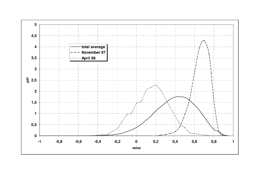
Figure 1: Distribution of matrix elements of the correlation matrix ${\bf C}$ (solid line) calculated from the daily price variation of all $N=30$ companies comprised by DAX. The solid line corresponds to an average over all time windows of length $T=30$ trading days during the period 1990-1999, the dashed line to an average over all such time windows which end during November 1-30, 1997 and the dotted line to an average over those which end during April 1-30, 1998.

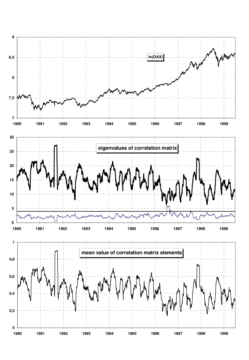
Figure 2: Upper panel: ln(DAX) during the period 1990-1999. Middle panel: Time-dependence of two largest eigenvalues corresponding to the DAX correlation matrix ${\bf C}$ calculated from the time-series of daily price changes in the interval of $T=30$ past days, during the years 1990-1999. $\lambda_{max}=4$ is indicated by the solid horizontal line. Lower panel: Time-dependence of the mean value of $\bf C$, which is a measure for the value of $\gamma$ in eq. (6), during the same period.

The rank of $\bf U$ is one and, consequently, the second term alone of the above equation develops exactly one nonzero eigenvalue of magnitude $\gamma$. Since the expansion coefficients of this particular state are all equal, this assigns a maximum of collectivity to such a state. If $\gamma$ is significantly larger than zero, the dominant structure of $\bf C$ is expected to be determined by this second term and $\bf G$ can be considered as just a ’noise’ correction. An anticipated result is that one collective eigenstate with a large eigenvalue is separated by a sizable gap from the remaining small eigenvalues.

3 Dynamics of DAX and Dow Jones

The study presented here is based on daily price variation of all the stocks of the Deutsche Aktienindex (DAX) and, independently, of the Dow Jones during the years 1990-1999. Both these markets involve the same number $(N=30)$ of the companies and, in this respect, are thus comparable. The time-dependence of correlations encoded in $\bf C$ can then be investigated by setting the time window $T=30$ ($T$ should not be smaller than $N$ as that would artificially reduce the rank of $\bf C$) and continuously moving it over the whole time period of interest. A clear indication that the character of correlations may nontrivially vary in time comes already from the distribution of entries of $\bf C$ recorded at different time intervals. Some examples of the corresponding probability functionals (pdf) for the DAX are shown in Fig. 1. In all the cases the distributions are Gaussian-like, but their variance and location is significantly different.

The middle panel of Fig. 2 shows the time-dependence of the two largest eigenvalues of the DAX correlation matrix. Their changes in time are strong indeed. However, already the second eigenvalue remains essentially all the time within the bounds prescribed by eq. (5) (in the present case $\lambda^{max}=4$). It is interesting to relate the largest eigenvalue $(\lambda_{1})$ to the global index (upper panel). As it is quite clearly seen, the global increases and decreases, respectively, are governed by dynamics of significantly distinct nature. The decreases are always dominated by one strongly collective eigenvalue. By conservation of the trace of $\bf C$ the remaining eigenvalues are then suppressed. The opposite applies to the increases; their propagation is always less collective. This can be concluded from the fact that the largest eigenvalue moves down and this move down is compensated by a simultaneous elevation of the lower eigenvalues. It is also very interesting to notice that the interpretation of these results in terms of eq. (6) is of an amazing accuracy. The lower panel of Fig. 2 shows the time-dependence of the mean value of $\bf C$, the quantity which provides a measure of $\gamma$. Any differences between the two lines (middle and lower panel) can hardly be detected.

Another quantity, oriented more towards characterising the localization properties of eigenvectors, originates from the information entropy $I_{\alpha}$ of an eigenvector ${\bf v}^{\alpha}$, defined by its components as

$$I_{\alpha}=-\sum_{i=1}^{N}(v^{\alpha}_{i})^{2}\ln(v^{\alpha}_{i})^{2}.$$ (7)

Using this quantity we then determine a degree of localization

$$L_{\alpha}=\exp(I_{\alpha}).$$ (8)

In the case of uniform distribution $(v^{\alpha}_{i}=1/\sqrt{N})$ it yields $L_{\alpha}=N$, i.e., the eigenstate is maximally delocalized. Another relevant limit is the one which corresponds to a Gaussian orthogonal ensemble (GOE) of random matrices. In this case $I_{\alpha}^{GOE}=\psi(N/2+1)-\psi(3/2)$ (Izrailev 1990), where $\psi$ is the digamma function. In our case of $N=30$ this gives $I^{GOE}\approx 2.67$ and thus $L^{GOE}\approx 14.44$.

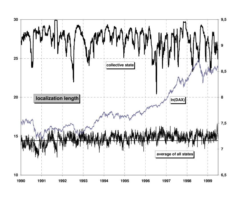
Figure 3: Time-dependence of the localization length for the most collective state and for the average over all the states. The solid horizontal line at $L\approx 14.44$ corresponds to the Gaussian orthogonal ensemble (GOE) limit and $L=30$ corresponds to a uniformly distributed eigenvector. In this plot the left vertical axis scale relates to the localization length, whereas the right axis scale belongs to the logarithm of the DAX index.

The two related localization lengths are shown in Fig. 3.The upper line corresponds to the collective state and the lower one to the average taken over all the $I_{\alpha}$’s. As one can see, it happens only during decreases that the dynamics of the most collective state approaches the most delocalized form. Otherwise this state becomes more localized. At the same time the localization length $\langle L\rangle$ corresponding to $\langle I_{\alpha}\rangle$ oscillates around its GOE limit. A more careful inspection shows, however, quite systematic deviations. Interestingly, on average, $\langle L\rangle$ moves in opposite direction relative to $I_{1}$, even though this most collective state is included in $\langle L\rangle$. This indicates that the stock market drawups lead to an increase of a global localization length and corrections of the stock market reduce it. This provides another argument in favour of interpreting the stock market changes from an increasing to decreasing phase as analogs of second order phase transitions (Drożdż et al. 1999).

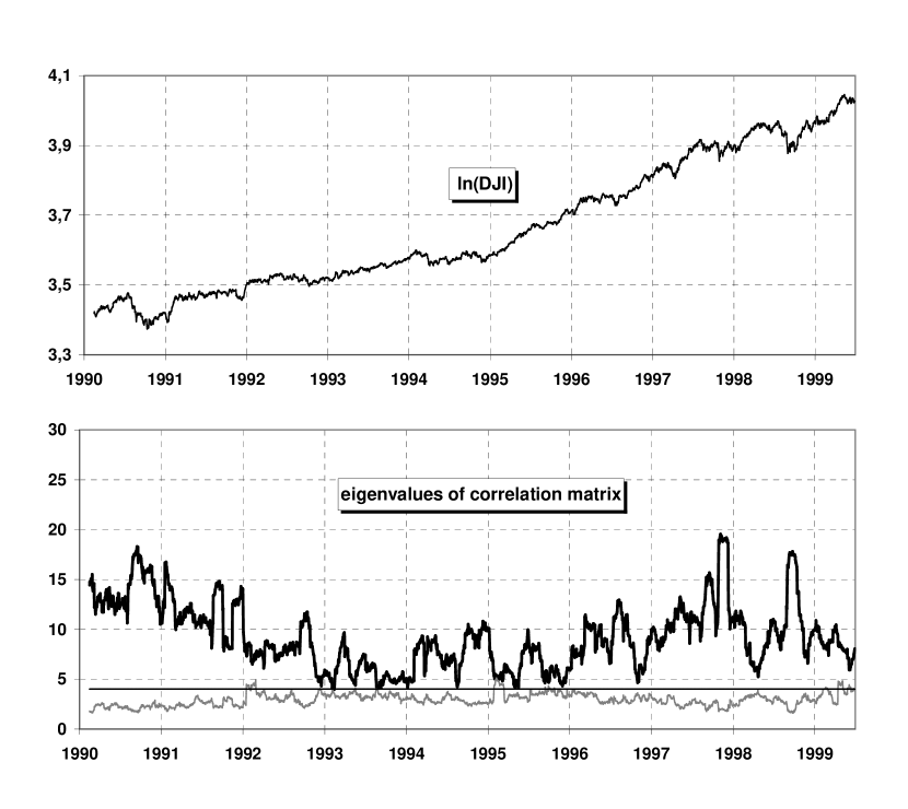
Figure 4: Same as the two upper panels of Fig. 2 but now for the Dow Jones.

Similar conclusions can be drawn form an analogous study of correlations amoung all the Dow Jones companies. One interesting difference is that on avarage the dynamics is here less collective. The magnitude of the separation between the largest eigenvalue and the remaining ones is systematically smaller for the Dow Jones than for the DAX, as can be easily seen by comparing Fig. 4 to Fig. 2.

4 DAX versus Dow Jones cross-correlations

All the above mentioned results are based on studies of single stock markets, in isolation to all others. In view of an increasing role of effects connected with the world globalization which, as every day experience indicates, seems to affect also the financial world, it is of great interest to quantify the related characteristics. Below we therefore study the cross-correlations between all the stocks comprised by DAX and by Dow Jones. Mixing them up results in 60 companies which determines the size of the correlation matrix to be studied. Consequently the time window $T=60$ is also used.

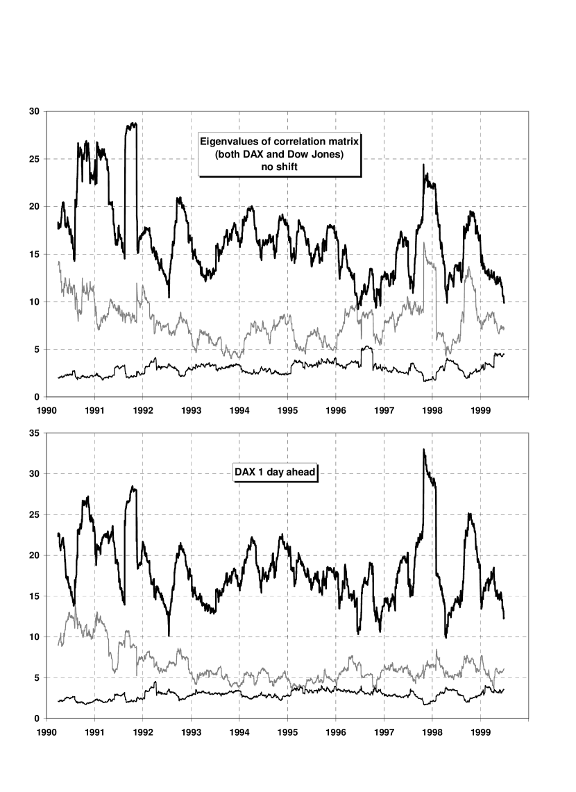
Figure 5: Upper panel: Time-dependence of three largest eigenvalues corresponding to the global (DAX + Dow Jones) correlation matrix ${\bf C}_{\cal G}$ calculated from the time-series of daily price changes in the interval of $T=60$ past trading days. Lower panel: Same as above but here the DAX returns are taken one day ahead relative to the Dow Jones returns when ${\bf C}^{\cal G}$ is constructed.

In our specific case of the two stock markets the corresponding global $({\cal G})$ correlation matrix ${\bf C}^{\cal G}$ can be considered to have the following block structure:

$${\bf C}^{\cal G}=\left(\matrix{{\bf C}^{DAX,DAX}&{\bf C}^{DAX,DJ}\cr{\bf C}^{DJ,DAX}&{\bf C}^{DJ,DJ}}\right)$$ (9)

The time-dependence of the resulting three largest eigenvalues of ${\bf C}^{\cal G}$ is illustrated in the upper panel of Fig. 5. In contrast to a single stock market case where the dynamics is typically dominated by one outlying eigenvalue here one can systematically identify two large eigenvalues. Both of them are always above the range of variation of the remaining eigenvalues which stay confined to the limits (eq. 5) prescribed by entirely random correlations $(\lambda^{max}=4)$.

In fact the two largest eigenvalues represent the two stock markets as if they were largely independent. The time-dependences of the largest eigenvalue $\lambda^{\cal G}_{1}$ of ${\bf C}^{\cal G}$ and of the largest eigenvalue $\lambda^{DAX}_{1}$ of ${\bf C}^{DAX,DAX}$ approximately coincide. The same applies to the second largest eigenvalue $\lambda^{\cal G}_{2}$ of ${\bf C}^{\cal G}$ when compared to the largest eigenvalue $\lambda^{DJ}_{1}$ of ${\bf C}^{DJ,DJ}$. No explicit documentation is necessary, since this already can be seen by comparing the present eigenvalues to those of Figs. 2 (middle panel) and 4 (lower panel).

The above thus indicates that the two sectors represented by ${\bf C}^{DAX,DAX}$ and by ${\bf C}^{DJ,DJ}$ respectively, remain practically disconnected. Such a conclusion, however, is somewhat embarrassing, because at the same time $\lambda^{\cal G}_{1}$ and $\lambda^{\cal G}_{2}$ (similarly as $\lambda^{DAX}_{1}$ and $\lambda^{DJ}_{1}$) go in parallel as far as their time-dependence is concerned, especialy over the last few years. Also the DAX and the Dow Jones increases and decreases, respectively, display significant correlations. Both these facts point to some sizeable correlations between the two markets. These become evident when the correlation matrix ${\bf C}^{\cal G}$ is calculated from $x_{j}^{DJ}(t)$ and $x_{i}^{DAX}(t+1)$, i.e., the DAX returns are taken one day advanced relative to the Dow Jones returns. The resulting time-dependence of the three largest eigenvalues is shown in the lower panel of Fig. 5. Now, except for the early 90’s, one large eigenvalue dominates the dynamics. This means that a sort of a single common market emerges. Moreover, this common market also obeys the characteristics observed before for the single markets. The collectivity of the dynamics is weaker (smaller $\lambda_{1}^{\cal G}$) during increases than during decreases.

5 Summary

In summary, the correlation matrix analysis of the stock market evolution allows to quantify the co-existence of collectivity and noise and shows that both are present. The majority of eigenvalues falls into limits prescribed by random matrix theory. The largest one, however, represents a collective state, whose time dependence provides arguments for a distinct nature of the mechanism governing financial increases and decreases, respectively. The increases are less collective by involving more competition as compared to decreases. Such characteristics can even be identified for a newly emerging global market in which the Dow Jones seems to be leading.

6 Acknowledgement

We are grateful to the organizers of the Symposium for their invitation. We thank the Symposium sponsors for financial support.

References

- [1] Drożdż S, Ruf F, Speth J, Wójcik M (1999) Imprints of log-periodic self-similarity in the stock market. Eur. Phys. J. B 10:589
- [2] Drożdż S, Grümmer F, Górski A, Ruf F, Speth J (2000) Dynamics of competition between collectivity and noise in the stock market. Physica A 287:440
- [3] Elton EJ, Gruber MJ (1995) Modern Portfolio Theory and Investment Analysis. Wiley J and Sons, New York
- [4] Izrailev FM (1990) Simple models of quantum chaos: spectrum and eigenfunctions. Phys. Rep. 196:299
- [5] Laloux L, Cizeau P, Bouchaud J-P, Potters M (1999) Noise dressing of financial correlation matrices. Phys. Rev. Lett. 83:1467
- [6] Markowitz H, (1959) Portfolio Selection: Efficient Diversification of Investments. Wiley J and Sons, New York
- [7] Mehta ML (1991) Random Matrices. Academic Press, Boston
- [8] Plerou V, Gopikrishnan P, Rosenow B, Amaral LAN, Stanley HE (1999) Universal and nonuniversal properties of cross-correlations in financial time-series. Phys. Rev. Lett. 83:1471
- [9] Sengupta AM, Mitra PP (1999) Distribution of singular values for some random matrices. Phys. Rev. E60:3389
Index
- abstract *