Continuous phase transition in polydisperse hard-sphere mixture

Abstract

In a previous paper (J. Zhang et al., J. Chem. Phys. 110, 5318 (1999)) we introduced a model for polydisperse hard sphere mixtures that is able to adjust its particle-size distribution. Here we give the explanation of the questions that arose in the previous description and present a consistent theory of the phase transition in this system, based on the Percus-Yevick equation of state. The transition is continuous, and like Bose-Einstein condensation a macroscopic aggregate is formed due to the microscopic interactions. A BMCSL-like treatment leads to the same conclusion with slightly more accurate predictions.

I Introduction

Monodisperse colloidal suspensions are rare in nature. Whether these colloidal particles are artificially prepared or not, in the best case the particle-size distribution is a narrow distribution around an average size. It is obvious that such a polydisperse nature will influence the physics and properties of these systems, and one could imagine that by the use of truly asymmetric mixtures it is possible to create systems with a behavior that cannot be described by the simple monodisperse-like approximation.

Conceptually we can distinguish between two types of polydispersity. One of them, which we could refer to as ‘intrinsic polydispersity’, arises from the fact that the particles present in the system are different by construction (in size, charge, or any other feature) and their characteristics are not changed by the interaction with other particles. This kind of systems are like multicomponent mixtures in which, at least in principle, the composition can be externally imposed. The new phenomenology that we can expect from this systems has its origin in fractionations into phases with different compositions [1, 2, 3, 4] (constrained by particle conservation) and their coupling with other transitions already present in the monodisperse system [5, 6].

The second kind of polydispersity can be found in self-assembling systems [7] (surfactants forming micelles, monomers forming chains, vesicles, etc). The aggregates present in these systems can be identified as the particles, each with different size, shape, conformation, etc; the difference with the intrinsically polydisperse systems being that the composition is determined by the chemical equilibrium between the constituents of the aggregates. As a consequence the equilibrium is not constrained by conservation of the number of particles and therefore no fractionation is to be expected. In principle the system can compensate losses of entropy by adjusting its composition. There are, however, other constraints in the system (the number of small constituents, for instance) and these may induce new kinds of transitions characterized by the appearance of one or a few macroscopic aggregates. As such can be cataloged phenomena as the appearance of lamellar and columnar phases in surfactant solutions [8, 9], emulsification failure in micro-emulsions [10, 11] or long chain formation in polymer solutions [12].

A study of polydisperse mixtures of either type is far from trivial. In the case of intrinsic polydispersity there is the experimental problem of how to fabricate colloidal particles according to a given particle-size distribution. Although in simulations this seems to be somewhat better under control, one easily could run into the problem of finite size effects due to an insufficient or inadequate sampling of particle sizes. This is not the case in self-assembling systems, although experimentally, their polydispersity cannot be easily characterized.

Theoretical descriptions of polydisperse systems are mainly based on a small set of moments of the particle-size distribution [3, 4, 13, 14, 15, 16] and it is assumed that mixtures with the same set of moments show a corresponding behavior. This seems to be a rather successful approach, although it is not obvious that could still be applied to very asymmetric mixtures.

In two previous articles we analyzed the behavior of idealized versions of polydisperse mixtures. The system was assumed to be composed of $N$ spherical aggregates which only interact via hard-core repulsion. The chemical equilibrium of the underlying constituents is accounted for by allowing particles to exchange size in such a way that the total volume [17] (compact aggregates) or surface [18] (surfactant micellar membranes) of the particles remains fixed at all times and the number of particles is constant.

Under the influence of the applied pressure the particle-size distribution of these systems changes. In the case of the constrained surface, the particle-size distribution changed from an exponentially decaying function in the low density limit to a single peaked distribution in the denser liquid phase. For sufficiently high pressures this system can form a number of different mechanically stable crystals, a monodisperse face-centered-cubic crystal, or a bidisperse $AB$ or $AB_{2}$ crystal.

For the system with the constraint on the total volume of the particles, it was found by theory and simulations that at a rather low volume fraction of approximately $0.26$ the system could no longer be described by Percus-Yevick type of equation of state, due to the formation of macroscopically large particles. In the present work we will show that this phenomenon is a true phase transition and provide a self-consistent theory for this sort of system. The nature of this transition has recently been studied in ideal systems [19] and found to be connected to Bose-Einstein condensation, and from this work we can conclude that interaction only changes the details, not the essential features. The connection of the present model with Bose-Einstein condensation was earlier suggested by D. Frenkel [20].

The remainder of this paper is organized as follows. In Sec. II we will show the results of computer simulations we have performed, and explain some of the details involved. These results are compared with a theory based on the Percus-Yevick equation of state in Sec. III. As we show in Sec. IV the treatment based on the heuristic BMCSL equation of state, leads to a slightly better theoretical description. In Sec. V we finish with a brief discussion on some of the issues raised in this paper.

II Simulations

The system under consideration here is one formed by $N$ spherical particles with different sizes. These particles are only interacting via a hard-core repulsion, and hence temperature is not a relevant parameter. We allow, however, pairs of particles to exchange volume under the constraint that the total volume occupied by all particles remains fixed. As a consequence the system has the freedom to explore different size-distribution functions and relax to the “optimal” one. In the previous work [17] we found by computer simulations that beyond a relative small pressure or density, some of the particles became macroscopically large. From theoretical arguments an upper bound to the pressure was obtained for fixed volume fraction, above which a single size distribution is unstable. However, simulations indicated a discrepancy with this result.

The formation of macroscopic particles (in simulations of the size of the simulation volume) beyond a critical value [19] is in fact comparable to Bose-Einstein condensation, or alternatively as a sort of sedimentation. In order to describe and simulate this phenomenon in our system in a correct manner, one has to eliminate the finite size effects that originate from the relative small number (typically of the order 1000) of particles that is being used in computer simulations. This could easily be solved by increasing the number of particles by one or several orders of magnitude, but this is seldom a preferred option. Moreover, in this particular case there exists a much more elegant solution to the problem.

The introduction of huge particles in a sea of smaller ones has two effects. The first is the reduction of the available volume that can be occupied by the smaller ones, and the second is the introduction of a hard wall formed by the big particles. It turns out that it is the second effect that caused the discrepancy between the simulation results and the upper bound of the equation of state [17]. The natural solution is therefore to eliminate this particular effect, which can be done by extracting the big particle(s) out of the simulation box.

We will assume that there is only a single big particle (aggregate) with a volume $V_{0}\geq 0$, but it can easily be extended to include several aggregates, albeit their number with respect to the simulation is not relevant. The total volume that can be occupied by the $N$ particles plus the aggregate, is denoted by $V_{f}=V_{0}+N\frac{\pi}{6}\langle\sigma^{3}\rangle=N\frac{\pi}{6}\sigma_{f}^{3}$, where $\langle\sigma^{3}\rangle$ is the average diameter cubed of the particles and $\sigma_{f}$ defines a natural length scale. The choice of $\sigma_{f}$ in this formulation is based on the infinite dilute system for which the size of the aggregate is zero. The volume that is accessible to the particles is denoted by $V$. But since we have extracted the aggregate out of the system the total thermodynamical volume of the system is given by $V_{T}=V+V_{0}$.

On this system we have performed Monte Carlo (MC) simulations using the isothermal-isobaric constant ($NPT$) ensemble. For a detailed description on Monte Carlo simulations we refer the reader to Ref. [21]; here we will only list the main features. As positional order will play no role, we will assume the simulation volume $V$ to be cubic and we will be using four different types of moves.

The first and simplest move is randomly selecting a particle and displacing it isotropically. The second type of move was introduced before [17]. It selects randomly a pair of particles and attempts to exchange a finite amount of volume, by adding this to one, and subtracting it from the other particle. Hereafter their new volumes are used in order to obtain the appropriate diameters. Obviously, if this process led to a negative volume, the move could not be accepted. Apart from that, both moves are accepted provided that no overlap is caused by these changes. Moreover, the amount of displacements and volume exchanges are drawn homogeneously from an interval, of which the size is continously adjusted in order to obtain an average acceptance per move between 35-50%.

In the third move we allow the simulation box to shrink or expand isotropically, in order for the system to equilibrate with respect to the applied pressure. This is in principle also a standard move in MC simulations using the $NPT$ ensemble. However, in this case it is required to modify the acceptance criterion of this move. This is caused by the fact that the thermodynamical volume $V_{T}$ and the volume of the simulation box $V$, although related, are not identical.

The weight of any non-overlapping configuration in the $NPT$-ensemble is proportional to $\exp(-\beta PV_{T})$, where $\beta=1/(k_{B}T)$ the inverse temperature. In addition to that, there is in MC-simulations a correction factor $V^{N}$ due to the use of scaled coordinates in order to facilitate the volume moves and periodic boundary conditions. As a result the volume move, if no overlaps are produced, is accepted with the probability

$$\mbox{Min}(1,\exp[\beta P(V_{T}^{(n)}-V_{T}^{(o)})-N\log(V^{(n)}/V^{(o)})]),$$ (1)

where the labels $n$ and $o$ refer to the new and old configuration respectively.

The fourth type of move is the exchange of volume between a particle and the aggregate. Although this seems to be equivalent to the volume exchange between particles, there is a subtle difference. Provided that no overlap is produced and both volumes remain positive this move is allowed. However, if the aggregate changes its volume, this results in a change of the available volume $V$ for the $N$ particles, while the thermodynamic volume $V_{T}$ remains fixed. As a result this move needs to be accepted with probability

$$\mbox{Min}(1,\exp[-N\log(V^{(n)}/V^{(o)})]).$$ (2)

We have performed a series of simulations on this system with $N=1000$ particles. In each simulation run we used $10^{5}$ sweeps, where in each sweep on average we try $N$ particle moves, $N/2$ volume exchanges, 1 volume move, and 5 exchanges of volume between the aggregate and one of the normal particles. Average quantities where obtained from a single run after equilibrium was reached. The time required to reach equilibrium strongly depends on the initial configuration. In simulations where an equilibrium configuration of a slightly higher or lower applied pressure is used, usually one run is sufficient. If started from a monodisperse simple cubic lattice, one or several runs are required, depending on the initial choice of the size of the aggregate and volume of the simulation box.

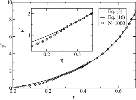
FIG. 1.: Equation of state. The solid and dotted line are the theoretical predictions above and below the transition respectively. The points are obtained from MC simulations on a 1000 particle system. The inset shows en enlargement of the transition point.

The results of the equation of state are shown in Fig. 1, where the the reduced pressure $P^{*}=\beta P\sigma_{f}^{3}$ is plotted as a function of the volume fraction $\eta=V_{f}/V_{T}$. The results obtained from expansion and compression runs, as well as started from monodisperse systems, all lead, within the estimated errors, to the same results. Near the volume fraction 0.26, where the critical value was found [17], a change in slope can be observed.

A natural order parameter for this system is the relative amount of fixed total volume of the particles found in the aggregate $V_{0}/V_{f}$ and is shown in Fig. 2. Comparison with simulations on systems with less particles and the absence of hysteresis in the equation of state suggests the possibility of a continuous phase transition.

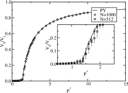
FIG. 2.: The solid line is the theoretical prediction of the order parameter $V_{0}/V_{f}$. The circles are results of MC-simulations on a 1000 particles system. The inset shows an enlargement of the area near the phase transition and in addition simulation results of a 512 particle system are indicated by squares.

The simulation results below the critical value are consistent with those obtained previously [17]. Above this value the results are different. The presence of the aggregate seems to prevent the formation of other macroscopic particles. Note that the difference is not so much the fact that there is a aggregate, but the way it is treated as an external buffer, thus eliminating the surface effects.

III Percus-Yevick Theory

In order to describe the system under consideration theoretically, one should realize that the presence of a thermodynamic volume $V_{T}$ as well as an available volume $V$ for the particles should carefully be taken into account. The system can be described by a polydisperse system of $N$ hard spheres in a volume $V$, which is in contact with an external bath, because in addition to the exchange of volume between the particles themselves, this can also be done with this bath or aggregate.

We will describe the polydisperse system within the Percus-Yevick approximation of a polydisperse hard-sphere mixture [22], from which the equation of state yields

$$\frac{\pi}{6}\beta P=\frac{\xi_{0}}{1-\xi_{3}}+\frac{3\xi_{1}\xi_{2}}{(1-\xi_{3})^{2}}+\frac{3\xi_{2}^{3}}{(1-\xi_{3})^{3}},$$ (3)

where $\xi_{k}$ is the $k$th moment of the particle-size distribution function

$$\xi_{k}=\frac{\pi}{6}\rho\int dvW(v)\sigma^{k}=\frac{\eta}{1-\frac{V_{0}}{V_{f}}\eta}\frac{\langle\sigma^{k}\rangle}{\sigma_{f}^{3}}.$$ (4)

Here $\rho=N/V$ is the number density defined with respect to the available volume, $\eta=V_{f}/V_{T}$ the volume fraction, and $W(v)$ is the continuous particle-size distribution function, which due to the type of interaction, is a function of the particle volume $v$. The Helmholtz free energy functional $F(N,V_{T},T)$ of this system, however, is a function of the thermodynamic volume $V_{T}$

$$\frac{\beta F}{N}=\log(\rho\Lambda^{3})-1+\int dvW(v)\log W(v)+\frac{\beta F^{ex}}{N},$$ (5)

where the excess free energy per particle is given by

$$\frac{\beta F^{ex}}{N}=-\log(1-\xi_{3})+\frac{3\xi_{1}\xi_{2}}{\xi_{0}(1-\xi_{3})}+\frac{3\xi_{2}^{3}}{2\xi_{0}(1-\xi_{3})^{2}}.$$ (6)

In order to obtain the equilibrium distribution, $W(v)$, we need to minimize this free energy functional, taking into account that there are two constraints which need to be satisfied. This is solved by adding the following two terms to the free energy functional

$$-{\cal L}_{0}\int dvW(v)-{\cal L}_{3}\left(\int dvW(v)v+\frac{V_{0}}{N}\right),$$ (7)

where ${\cal L}_{0}$ and ${\cal L}_{3}$ are Lagrange multipliers. The first term is due to the requirement that the particle-size distribution function should be normalized to unity, and the second is that the combined volume of all particles and the aggregate is fixed to be $V_{f}$.

The equilibrium particle-size distribution can now be obtained by minimizing the free energy functional with respect to $W(v)$ and the free parameter $V_{0}$. Stationarity with respect to changes in $W(v)$ leads to

$$\log(W(v))-\log(1-\xi_{3})+\frac{3\xi_{2}}{(1-\xi_{3})}\sigma+$$ (8)

$$\left(\frac{3\xi_{1}}{(1-\xi_{3})}+\frac{9\xi_{2}^{2}}{2(1-\xi_{3})^{2}}\right)\sigma^{2}+\frac{\pi}{6}\beta P\sigma^{3}-{\cal L}_{0}-{\cal L}_{3}\frac{\pi}{6}\sigma^{3}=0,$$ (9)

from which we can immediately derive the functional form of the function $W(v)$ that will minimize the free energy

$$W(v)=\exp\left(\sum_{i=0}^{3}\alpha_{i}\sigma^{i}\right),$$ (10)

where the coefficients $\alpha_{i}$ are determined by

$$\alpha_{1}=-\frac{3\xi_{2}}{(1-\xi_{3})},$$ (11)

$$\alpha_{2}=-\left(\frac{3\xi_{1}}{(1-\xi_{3})}+\frac{9\xi_{2}^{2}}{2(1-\xi_{3})^{2}}\right).$$ (12)

The values of $\alpha_{3}$ and $\alpha_{0}$ are fixed by the constraint on the total combined volume of the particles and the aggregate, and the normalization of the particle size-distribution, respectively. Formally, however, the coefficient $\alpha_{3}$ is given by

$$\alpha_{3}=-\frac{\pi}{6}(\beta P-{\cal L}_{3}).$$ (13)

In addition to these equations we have to minimize with respect to the volume of the aggregate. Note that the $\xi_{i}$ depend on the value of $V_{0}$ through the number density. Therefore we obtain

$$\frac{\partial\beta F}{\partial V_{0}}=-\frac{\partial\beta F}{\partial V_{T}}-{\cal L}_{3}=\beta P-{\cal L}_{3}=0.$$ (14)

This result does not automatically imply that $\alpha_{3}=0$. The reason is that we have to minimize the free energy with respect to the volume of the aggregate under the additional condition that the aggregate has a non-negative volume. As a consequence this can result in the possibility that the minimum is found for $V_{0}=0$ and the stationarity equation (14) not being satisfied. This leads to a natural splitting of the behavior of this system. For low pressures the volume of the aggregate will be zero, and the particle size-distribution is the exponential of a third order polynomial in the particle diameter. On increasing the pressure the coefficient $\alpha_{3}$, which can only be non-positive in order to allow a proper normalization, goes to zero. In this region the behavior is as explained before [17]. According to the theoretical description in the Percus-Yevick approximation, the coefficient $\alpha_{3}$ becomes zero at volume fraction $\eta=0.260198$ pressure $P^{*}=1.343442$. At this point the value $V_{0}=0$ not only minimizes the free energy, but also satisfies the stationarity equation (14). For pressures larger than this value the stationarity equation can always be satisfied with a positive volume for the aggregate and hence the coefficient $\alpha_{3}$ remains zero.

It turns out that this point is the location of a continuous transition. Beyond this point the system relaxes by transferring volume to the aggregate, and effectively scaling the polydisperse system to a smaller size. If we denote by a script $c$ the values of the critical system, this can be shown in the following way. If we replace the coefficients $\alpha_{k}$ in the particle size-distribution by $q^{k}\alpha_{ck}$, where $q$ is a positive number, and fix $\alpha_{0}$ by the normalization to unity, it follows directly from the special form (10) of $W(v)$ that the moments of the size-distribution are given by $\langle\sigma^{k}\rangle=\langle\sigma^{k}\rangle_{c}/q^{k}$. This results in

$$\alpha_{1}=-q^{3}\frac{3\eta_{c}}{(1-\eta_{c})}\frac{\langle\sigma^{2}\rangle}{\sigma_{f}^{3}},$$ (15)

and provided that $q$ is determined by

$$q^{3}=\frac{\eta}{1-\eta}\frac{1-\eta_{c}}{\eta_{c}}$$ (16)

this is a solution of Eq. (11). Applying this procedure to $\alpha_{2}$ leads to the same expression for $q$. Therefore the scaled size-distribution function leads to a minimum free energy, albeit for a different applied pressure.

The pressure equation of state beyond the critical point also becomes fairly simple now. If we rewrite the pressure (3) using the solutions (11) and (12), we obtain

$$\frac{\pi}{6}P^{*}=\frac{\xi_{0}-\frac{1}{3}\alpha_{1}\xi_{1}-\frac{2}{3}\alpha_{2}\xi_{2}}{1-\xi_{3}}\sigma_{f}^{3}=\frac{2\eta}{1-\eta},$$ (17)

where we used that if $\alpha_{3}=0$ the functional form of $W(v)$ leads to the identity $3\langle\sigma^{0}\rangle+\alpha_{1}\langle\sigma\rangle+2\alpha_{2}\langle\sigma^{2}\rangle=0$. We can also derive a simple expression for the order parameter $V_{0}/V_{f}$ of the system

$$\frac{V_{0}}{V_{f}}=1-\frac{\langle\sigma^{3}\rangle}{\sigma_{f}^{3}}=1-\frac{P^{*}_{c}}{P^{*}}.$$ (18)

The curves of the equation of state and the order parameter are shown in Figs. 1 and 2 respectively, and show a perfect agreement with the simulation results. In Fig. 1 the dotted line represents the equation of state below the transition, i.e. Eq. (3), while the solid line is the one above as given by Eq. (17). The later one is extended to the zero density limit in order to visualize the difference between both branches.

From these results two additional illustrative properties can be derived for the system beyond the point of the transition. Using that the particle size-distribution only changes according to a dimensional scaling or from the order parameter (18), we find that

$$P\langle\sigma^{3}\rangle=P_{c}\sigma_{f}^{3}.$$ (19)

This simply states that the system becomes scale invariant, with a constant pressure if it is defined in terms of the average particle volume. The other result is that $\xi_{3}$, which can be identified with the local volume fraction of the particles, remains fixed, i.e. $\xi_{3}=\eta_{c}$. These results can be used in order to determine the point of transition from simulations. This is illustrated in Fig. 3, where $P^{*}\langle\sigma^{3}\rangle/\sigma_{f}^{3}$ as a function of $\eta$, and the applied pressure $P^{*}$ as a function of $\xi_{3}$ are shown, as measured in our MC-simulations. According to these simulations the transition is found at a volume fraction $\eta=0.2623\pm 0.0003$ and pressure $P^{*}=1.360\pm 0.003$.

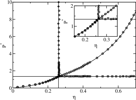
FIG. 3.: Comparison of the simulation results for a 1000 particles system with the theoretical predictions. The circles represent the applied pressure $P^{*}$ as function of the volume fraction $\eta$. The squares the local pressure $P^{*}\langle\sigma^{3}\rangle/\sigma_{f}^{3}$ as function of $\eta$, and the diamonds the applied pressure $P^{*}$ as function of the local volume fraction $N\langle v\rangle/V$.

The prediction of the particle size-distribution $W(v)$ is compared with the simulation results in Fig.4. By plotting $\mbox{ln}(W(v)/P^{*})$ as a function of $P^{*}v$, the distributions above the transition coincide and agree perfectly with the predicted curve from Percus-Yevick. The discrepancy at higher values for $P^{*}v$ is merely a consequence of an insufficient sampling of the largest particles in the system. For $P^{*}=1.50$, there is the additional effect that this is close to the transition, where the system tends to probe larger particles.

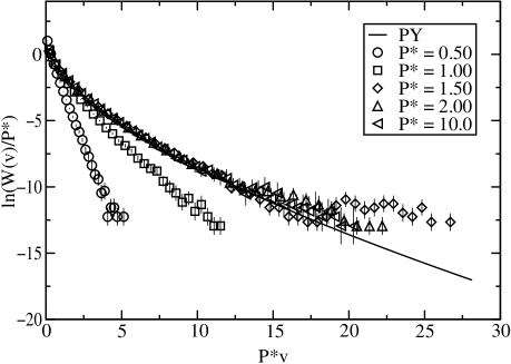
FIG. 4.: The particles size-distributions are shown by plotting $\mbox{ln}(W(v)/P^{*})$ as a function of $P^{*}v$. Due to this scaling all distributions above the transition should coincide, without using the actual values of the pressure and volume fraction at the transition. The solid curve is the predicted curve by the Percus-Yevick approach.

It turns out that within the Percus-Yevick approximation the system shows a continuous phase transition, which is characterized by the non-zero volume of a aggregate. In fact it shows some similarities to Bose-Einstein condensation, because what actually happens is that the interaction of microscopic particles leads to the formation of a macroscopic aggregate [19].

IV BMCSL-theory

It is a well known fact that the Percus-Yevick equation of state in a monodisperse hard sphere system can be improved by combining it with the virial equation of state. This results in the Carnahan-Starling equation of state [23]. A similar approach can be made for polydisperse sphere mixtures, and the resulting heuristic equation of state is due to Boublík, Mansoori, Carnahan, Starling, and Leland (BMCSL) [24, 25]

$$\frac{\pi}{6}\beta P=\frac{\xi_{0}}{1-\xi_{3}}+\frac{3\xi_{1}\xi_{2}^{2}}{(1-\xi_{3})^{2}}+\frac{3\xi_{2}^{3}}{(1-\xi_{3})^{3}}-\frac{\xi_{3}\xi_{2}^{3}}{(1-\xi_{3})^{3}}.$$ (20)

A straightforward integration of this equation of state shows that the excess free energy up to a constant is given by [22]

$$\frac{\beta F^{ex}}{N} = \left(\frac{\xi_{2}^{3}}{\xi_{0}\xi_{3}^{2}}-1\right)\ln(1-\xi_{3})$$ (22)

$$+\frac{3\xi_{1}\xi_{2}}{\xi_{0}(1-\xi_{3})}+\frac{\xi_{2}^{3}}{\xi_{0}\xi_{3}(1-\xi_{3})^{2}}.$$

The additional constant is independent of the volume, but could in principle depend on the moments of the size-distribution, without changing the equation of state. Such a constant would be relevant for this particular model, since the size-distribution of the system can be changed, and therefore an additional change in free energy can be produced. From general applicability of the free energy functional to different models, however, it can be shown that this contribution necessarily vanishes.

We now can apply the same procedure as was used in the case of the Percus-Yevick approximation. The functional derivative of the free energy with respect to $W(v)$ leads to the same functional form (10) as before, but the stationarity equations on the coefficients $\alpha_{i}$ need to be modified

$$\alpha_{1}=-\frac{3\xi_{2}}{(1-\xi_{3})},$$ (23)

$$\alpha_{2}=-\frac{3\xi_{1}}{(1-\xi_{3})}-\frac{3\xi_{2}^{2}}{\xi_{3}(1-\xi_{3})^{2}}-\frac{3\xi_{2}^{2}}{\xi_{3}^{2}}\log(1-\xi_{3}),$$ (24)

$$\alpha_{3} = -\frac{\pi}{6}(\beta P-{\cal L}_{3})$$ (26)

$$+\left(\frac{\xi_{2}}{\xi_{3}}\right)^{3}\left[2\log(1-\xi_{3})+\frac{\xi_{3}(2-\xi_{3})}{(1-\xi_{3})}\right].$$

The derivative of the free energy with respect to the volume of the aggregate leads again to

$$\frac{\partial\beta F}{\partial V_{0}}=-\frac{\partial\beta F}{\partial V_{T}}-{\cal L}_{3}=(\beta P-{\cal L}_{3})=0.$$ (27)

The second term on the right hand side of Eq. (26) is, except in the zero density limit, always positive. As a consequence Eq. (27) can never be satisfied, because such a solution would lead to a positive $\alpha_{3}$ and hence a non-normalizable size-distribution function. The minimum free energy for given volume fraction will therefore not be a solution of all the stationarity equations simultaneously.

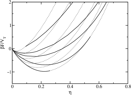
FIG. 5.: The Helmholtz free energy per volume as a function of the volume fraction for fixed order parameter $V_{0}/V_{f}$, i.e. constant size of the aggregate (solid curves) and for scaled distribution functions (dotted curves). Both sets are similar but use only a different parameter for characterization.

Since the stationarity equations (23) - (26) are directly related to the equations for chemical equilibrium between the different particle sizes, they need to be fulfilled. If we fixed the volume of the aggregate $V_{0}$, these equations would be sufficient to obtain the unique distribution function that minimizes the free energy. In Fig. 5 we have plotted the free energy per volume for several fixed values of $V_{0}$ (solid curves). On these curves the stationarity equations are satisfied, hence the value of $V_{0}$ that leads to the minimum free energy corresponds to the equilibrium situation. These curves are bounded by an lower and upper limit of the volume fraction. The lower limit corresponds to the case where $\alpha_{1}=\alpha_{2}=0$ and the upper limit corresponds to the case where $\alpha_{3}=0$. Outside this interval no self-consistent solution of the stationarity equations can be obtained.

Similar to what we found in the Percus-Yevick approach, we can scale the particle size-distribution function such that we obtain a solution to the stationarity equations for a different volume fraction by replacing $\alpha_{k}$ by $q^{k}\alpha_{k}$ and fixing the normalization constant. The free energy per volume for several of these scaled solutions is also shown in Fig. 5 as dotted curves. Both sets of curves are similar, but use a different parameter to describe them.

The equilibrium situation of our model is the one that corresponds to the lowest free energy for given volume fraction and will correspond to the envelope of the set of curves in Fig. 5. One can show that we have two regions, which is illustrated by this figure. Below the transition the equilibrium situation corresponds to the curve for which $V_{0}=0$, i.e. without a macroscopic aggregate. Above the transition we will follow the branch of a scaled solution, emerging from the end point of this curve determined by $\alpha_{3}=0$. The transition point is therefore obtained by self-consistently solving the case for $V_{0}=\alpha_{3}=0$ and leads to a volume fraction $\eta=0.262611$ and pressure $P^{*}=1.356275$.

Actually the same reasoning could have been used for the Percus-Yevick approach. But since for that case all stationarity equations could be solved simultaneously, there was no need to follow this line of argumentation.

The numerical predictions of the transition point for the BMCSL approach are slightly better in agreement with the simulation results than the results from Percus-Yevick. The difference between both predictions is however too small in order for it to be visible in any of the figures. In principle also the size-distribution function can be used to distinguish both theories, however, in order to do so the number of particles should be increased several orders of magnitudes in order to obtain sufficient statistics for the larger particles and to make the difference in the tail of the distribution visible.

V Discussion

We have demonstrated how to obtain a self-consistent theory for a polydisperse hard sphere system, where particles are able to change their size by exchanging volume. Within the Percus-Yevick approximation this system shows a continuous phase transition, in which the microscopic interactions lead to the formation of a macroscopic aggregate, a behavior similar to Bose-Einstein condensation. The theoretical results have been compared with a new series of computer simulations and show an excellent agreement, because in the new treatment we have eliminated the finite size effect that previously led to discrepancies between theory and simulation.

This peculiar system, which at best can be considered to be an extremely idealized version of spherical micelles, exposes an unusual behavior in the BMCSL-approach. The equilibrium state of the system is one which does not satisfies the stationarity equations but is determined by the boundary conditions on the problem, i.e. a normalizable particle size-distribution. Apart from that the difference between both approximations is minor and in order to determine which one is better, simulations would be required with several orders of magnitude more particles.

REFERENCES

- [1] R. P. Sear, Europhys. Lett. 44, 531 (1998).
- [2] P. Bartlett, J. Chem. Phys. 109, 10970 (1998).
- [3] J. A. Cuesta, Europhys. Lett. 46, 197 (1999).
- [4] P. B. Warren, Europhys. Lett. 46, 295 (1999).
- [5] P. Bartlett and P. B. Warren, Phys. Rev. Lett. 82, 1979 (1999).
- [6] M. A. Bates and D. Frenkel, J. Chem. Phys. 109, 6193 (1998).
- [7] W. M. Gelbart, A. Ben-Shaul, and D. Roux, eds., Micelles, Microemulsions and Monolayers (Springer-Verlag, New York, 1994).
- [8] N. Boden, R. J. Bushby, C. Hardy, and F. Sixl, Chem. Phys. Lett. 123, 359 (1986).
- [9] N. Boden, S. A. Corne, and K. W. Jolley, J. Phys. Chem. 91, 4092 (1987).
- [10] M. S. Leaver, U. Olsson, H. Wennerstrom, and R. Strey, J. Phys. II 4, 515 (1994).
- [11] D. Vollmer, R. Strey, and J. Vollmer, J. Chem. Phys. 107, 3619 (1997).
- [12] R. J. Petscheck, P. Pfeuty, and J. C. Wheeler, Phys. Rev. A 34, 2391 (1986).
- [13] P. Sollich and M. E. Cates, Phys. Rev. Lett. 80, 1365 (1998).
- [14] P. B. Warren, Phys. Rev. Lett. 80, 1369 (1998).
- [15] P. Sollich, P. B. Warren, and M. E. Cates, Adv. Chem. Phys. 116, 265 (2001).
- [16] N. Clarke, J. A. Cuesta, R. Sear, P. Sollich, and A. Speranza, J. Chem. Phys. 113, 5817 (2000).
- [17] J. Zhang, R. Blaak, E. Trizac, J. A. Cuesta, and D. Frenkel, J. Chem. Phys. 110, 5318 (1999).
- [18] R. Blaak, J. Chem. Phys. 112, 9041 (2000).
- [19] R. P. Sear and J. A. Cuesta, cond-mat/0012256 (2000).
- [20] D. Frenkel, Private Communication.
- [21] D. Frenkel and B. Smit, Understanding Molecular Simulation. From Algorithms to Applications (Academic Press, Boston, 1996).
- [22] J. J. Salacuse and G. Stell, J. Chem. Phys. 77, 3714 (1982).
- [23] N. F. Carnahan and K. E. Starling, J. Chem. Phys. 51, 635 (1969).
- [24] T. Boublík, J. Chem. Phys. 53, 471 (1970).
- [25] G. A. Mansoori, N. F. Carnahan, K. E. Starling, and T. W. Leland, Jr., J. Chem. Phys. 54, 1523 (1971).