Micellization in the presence of polyelectrolyte

Abstract

We present a simple model to study micellization of amphiphiles condensed on a rodlike polyion. Although the mean field theory leads to a first order micellization transition for sufficiently strong hydrophobic interactions, the simulations show that no such thermodynamic phase transition exists. Instead, the correlations between the condensed amphiphiles can result in a structure formation very similar to micelles.

I Introduction

Interaction between polyelectrolytes and ionic amphiphiles has attracted significant attention in both the molecular biology and the condensed matter physics communities [1, 2, 3, 4, 5, 6, 7, 8, 9, 10, 11, 12, 13]. The driving motivation for this surge in interest is the possible application of polyelectrolyte-amphiphile complexation in gene therapy [2]. One of the major stumbling blocks in designing a successful gene therapy is the lack of a transfection mechanism by which a DNA strand can be inserted into a cell [2]. The problem arises as a result of strong electrostatic repulsion between the DNA and the molecular membrane, both of which are negatively charged. This repulsion prevents a DNA segment from coming in contact with a cell membrane, thus precluding any possibility of transfection. To overcome the electrostatic repulsion a number of protocols have been developed. The most explored ones rely on genetically modified viral vectors. A number of complications which can arise from the viral gene therapy have stimulated a development of non-viral methods [2]. One such method explores the association between a negatively charged DNA and cationic lipids or surfactants. A particular method which has attracted much attention relies on formation of lipoplexes [3, 4, 5]. These are complexes composed of a DNA strand and cationic lipid vesicles. Unfortunately the non-viral methods are also prone to problems since, as is well known, the cationic surfactants and lipids are toxic to an organism [2]. An interesting question which then arises is what is the minimum concentration of cationic amphiphile needed to form a lipoplex or a surfoplex? This question is well posed, since it has been known for some time that the polyelectrolyte-ionic amphiphile complexation occurs in a cooperative manner [10, 11, 14, 15, 16]. It is, therefore, possible to identify the location of the cooperative condensation with the critical concentration needed to form complexes. What is the internal structure of such complexes? Are the condensed amphiphiles uniformly distributed along the DNA or do they form micellar aggregates on the surface of a polyion? As a first attempt to study this difficult problem we shall appeal to a very simple model [17, 18].

II The Model

We consider a rigid polyion modeled as a cylinder of length $Zb$ and radius $Rb$ inside a uniform medium of dielectric constant $\epsilon$. The total charge of a polyion, $-Zq$, is uniformly distributed along the length of the cylinder so that each one of the $Z$ monomers has charge $-q$. To further simplify the calculations, the longitudinal and angular degrees of freedom are discretized. The surface of the cylinder is subdivided into $Z$ parallel rings of $n$ sites each. The $m$ condensed amphiphiles are restricted to move between the $Zn$ ring sites, on the surface of the cylinder.

Each amphiphile has a charged head group and a hydrocarbon tail. For generality we shall take the head group to have charge $\alpha q$. The hardcore repulsion between the amphiphiles requires that each site is occupied by at most one amphiphile. For the specific case of DNA and dodecyltrimethyl amonium bromide (DoTAB) at the cooperative binding transition $m\approx 0.8Z$ [11, 14].

We define the occupation variables $\sigma_{ij}$, with $i=1,\ldots,Z$ and $j=1,\ldots,n$, in such a way that $\sigma_{ij}=1$ if a surfactant is attached at $j$’th ring position of the $i$’th monomer and $\sigma_{ij}=0$ otherwise. Since the number of amphiphiles is fixed, the values of occupation variables obey the constraint

$$\sum_{i=1}^{Z}\sum_{j=1}^{n}\sigma_{ij}=m\;.$$

The Hamiltonian for this model has the following contributions:

• Electrostatic surfactant-monomers interaction:

  $$\beta{\cal H}_{1}=-\alpha\xi\sum_{i,j=1}^{Z}\sum_{k=1}^{n}\frac{\sigma_{ik}}{\sqrt{R^{2}+(i-j)^{2}}},$$ (1)

where we have introduced a dimensionless charge density, the Manning parameter [19, 20, 21],

$$\xi\equiv\frac{\beta q^{2}}{b\epsilon}\;\;.$$ (2)

FIG. 1.: Interaction between a surfactant in the $i$’th ring with the $j$’th monomer. The distance between the surfactant and the monomer is $r=b\sqrt{R^{2}+(i-j)^{2}}$.

• Electrostatic surfactant-surfactant interaction:

  $$\beta{\cal H}_{2}=\frac{\alpha^{2}\xi}{2}\sum_{i,j=1}^{Z}\sum_{k,l=1}^{n}\frac{\sigma_{ik}\sigma_{jl}(1-\delta_{ij}\delta_{kl})}{\sqrt{(i-j)^{2}+4R^{2}\sin^{2}\left(\frac{\pi}{n}|k-l|\right)}}\;.$$ (3)

  

  FIG. 2.: Distance between a surfactant located on the $i$’th ring in the $k$’th position and the surfactant located on the $j$’th ring and the $l$’th position, $r=b\sqrt{(i-j)^{2}+4R^{2}\sin^{2}\left(\pi|k-l|/n\right)}$.

• Hydrophobic interactions between the hydrocarbon tails:

  $$\beta{\cal H}_{3}=-\chi\sum_{i=1}^{Z}\sum_{j=1}^{n}\sigma_{ij}\sigma_{i,j+1}-\chi\sum_{i=1}^{Z-1}\sum_{j}^{n}\sigma_{ij}\sigma_{i+1,j}\;\;,$$ (4)

where $\sigma_{i,n+1}=\sigma_{i1}$. The first term of Eq. (4) is due to the interactions between nearest neighbor amphiphiles on the same ring, while the second term is due the interactions between equivalent sites on consecutive rings. The hydrophobicity parameter $\chi$ can be related to the size of the amphiphiles alkyl chain [14].

The hydrophobic interactions between surfactant and water produce an effective attraction between the amphiphiles, forcing them to stick together. By doing so they expel the water molecules from their vicinity, lowering the overall free energy. The pairwise additive form of the hydrophobic interaction adopted in Eq. (4) is clearly an over simplification. Nevertheless, we expect that this simple expression will help shed some light on the structure of the polyion-amphiphile complexes.

III Mean Field Theory

To begin our study of the distribution of surfactants along the polyion we shall appeal to the mean field theory [22, 23]. A note of caution, however, must be raised. While the mean field theory is expected to work very well for Coulombic long ranged interactions, it might not be so successful with the short ranged hydrophobic forces. This is in particular so since the problem is intrinsically one dimensional, and the fluctuations associated with the short ranged hydrophobic interactions are expected to be significant [16]. With this note of caution in mind we shall proceed with the mean field study.

The Gibbs-Bogoliubov inequality puts an upper bound on the total free energy, ${\cal F}\leq{\cal F}_{0}+\langle{\cal H}-{\cal H}_{0}\rangle_{0}\equiv{\cal\overline{F}}$, where ${\cal F}_{0}$ is the free energy associated with the trial Hamiltonian ${\cal H}_{0}$. To perform the calculations we shall take ${\cal H}_{0}$ to be of a particularly simple one body form,

$${\cal H}_{0}=q\sum_{i}^{Z}\sum_{p}^{n}\phi_{ip}\sigma_{ip}\;.$$ (5)

The partition function associated with ${\cal H}_{0}$ can be calculated straight forwardly

$$Z_{0}=\sum_{\{\sigma\}}\exp\left\{-\beta q\sum_{i,p}\phi_{ip}\sigma_{ip}\right\}=\prod_{i,p}\left\{1+\exp\left(-\beta q\phi_{ip}\right)\right\}\;\;,$$ (6)

and the free energy is

$${\cal F}_{0}=-\frac{1}{\beta}\sum_{i,p}\ln\left\{1+\exp\left(-\beta q\phi_{ip}\right)\right\}\;\;.$$ (7)

The average occupation of site $p$ on the ring $i$, $\rho_{ip}\equiv<\sigma_{ip}>_{0}$, is then

$$\rho_{ip}=\frac{1}{1+e^{\beta q\phi_{ip}}}$$ (8)

or

$$\phi_{ip}=\frac{1}{\beta q}\ln\left(\frac{1-\rho_{ip}}{\rho_{ip}}\right)\;\;.$$ (9)

The free energy associated with ${\cal H}_{0}$ can be rewritten as

$${\cal F}_{0}=\frac{1}{\beta}\sum_{i,p}\ln(1-\rho_{ip})\;\;.$$ (10)

After evaluating the average of $\langle{\cal H}-{\cal H}_{0}\rangle_{0}$ with respect to ${\cal H}_{0}$, the upper bound to the total free energy becomes

$$\beta{\cal\overline{F}} = \sum_{i,j}\ln(1-\rho_{ij})-\alpha\xi\sum_{i,j}^{Z}\sum_{k}^{n}\frac{\rho_{ik}}{\sqrt{R^{2}+(i-j)^{2}}}+\frac{\alpha^{2}\xi}{2}\sum_{i,j}^{Z}\sum_{k,l}^{n}\frac{\rho_{ik}\rho_{jl}(1-\delta_{ij}\delta_{kl})}{\sqrt{(i-j)^{2}+4R^{2}\sin^{2}\left(\frac{\pi}{n}|k-l|\right)}}$$ (12)

$$-\chi\sum_{i}^{Z}\sum_{j}^{n}\rho_{ij}\rho_{i,j+1}-\chi\sum_{i=1}^{Z-1}\sum_{j}^{n}\rho_{ij}\rho_{i+1,j}-\sum_{i}^{Z}\sum_{j}^{n}\rho_{ij}\ln\left(\frac{1-\rho_{ij}}{\rho_{ij}}\right)\;\;.$$

To find the optimum upper bound, Eq. (12) must be minimized with respect to the average site occupation, leading to

$$\rho_{ij}=\frac{1}{1+e^{\beta(\varphi_{ij}+\mu)}}\;,$$ (13)

where $\mu$ is a Lagrange multiplier introduced to enforce the constraint $\sum_{i,j}\rho_{ij}=m$ and

$$\beta\varphi_{ij} = -\alpha\xi\sum_{k}^{Z}\frac{1}{\sqrt{R^{2}+(i-k)^{2}}}+\alpha^{2}\xi\sum_{k}^{Z}\sum_{l}^{n}\frac{\rho_{kl}(1-\delta_{ik}\delta_{jl})}{\sqrt{(i-k)^{2}+4R^{2}\sin^{2}\left(\frac{\pi}{n}|j-l|\right)}}$$ (15)

$$-\chi(\rho_{i,j-1}+\rho_{i,j+1})-\chi\left[(1-\delta_{iZ})\rho_{i+1,j}+(1-\delta_{i1})\rho_{i-1,j}\right]\;.$$

Using the constraint above, $\mu$ can be evaluated leading to a self consistent equation for the average site occupation,

$$\rho_{ij}=\frac{m}{m+\sum_{k,l}(1-\rho_{kl})e^{\beta(\varphi_{ij}-\varphi_{kl})}}\;\;.$$ (16)

Eq. (16) can be solved numerically to find the equilibrium amphiphile distribution along the polyion.

In Fig. 3 we show the average number amphiphiles per ring along the polyion for $\xi=4.17$ and $\chi=1$. We note that the amphiphiles are uniformly distributed along the polyion except at the ends of the macromolecule, where their density is strongly depleted.

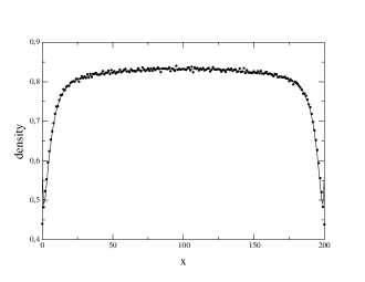
FIG. 3.: Comparison between the profiles predicted by the mean field theory and simulations results, for $\xi=4.17$, $\chi=1$, $Z=201$, $m=160$, and $n=5$.

For $\chi\approx 1.35$ a curious phenomenon occurs, as shown in Fig. 4. At this value of hydrophobicity the sites of the central ring become preferentially occupied by the amphiphiles. This corresponds to a micellization transition, in which the strong hydrophobic attraction between the surfactants overcomes entropy to produce a mesoscopic aggregate of amphiphiles. As $\chi$ increases, a number of other peaks appear. Within the mean field theory we find that the micellization transition is of first order. The fact that a short ranged interaction produces a first order transition in a pseudo one dimensional system should leave us concerned. To check the existence of this transition we have carried out a set of Monte-Carlo simulations (MC).

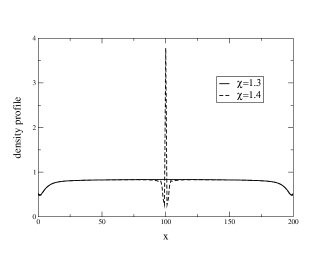
FIG. 4.: The mean field theory prediction for $\chi=$1.3 and 1.4, $\xi=4.17$, $Z=201$, $m=160$, $n=5$. The peak is an artifact of the mean field approximation.

IV Simulations

To simulate this model we use a standard Monte Carlo with particle-hole exchange, not restricted to nearest-neighbors pairs. The density profiles and the energy were measured after thermalization, results being both time and sample averaged. The simulations considered where done for DNA with $\xi=4.17$, $Z=201$, $n=160$, $m=5$ and various values of $\chi$. The averages were obtained using 100 samples.

For $\chi<1.35$ we find that the mean field theory is in excellent agreement with the MC. For $\chi>1.35$, on the other hand, the simulations do not find any evidence of the micellization transition present in mean field (see Fig. 5). The energy is a smooth function of $\chi$, with no indication of the first order micellization transition, Fig. 6. As expected, the short ranged hydrophobic interaction can not result in a phase transition in a one dimensional system.

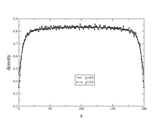
FIG. 5.: The Monte Carlo density profiles for $\chi=0$ and $\chi=5$ for a system with $\xi=4.17$, $Z=201$, $n=160$ and $m=5$. For $\chi=5$, the mean field theory predicts the existence of many peaks, that are absent in simulation.

In spite of the absence of a true phase transition, the correlations between the condensed amphiphiles can lead to formation of structures along the polyion. To study these, we have constructed a histogram of amphiphile cluster sizes within the Monte Carlo simulation. Here the size of a cluster is defined by the number of amphiphiles per ring. Fig. 7 shows that for amphiphiles with short alkyl tails (small hydrophobicity) the clusters are composed of only one amphiphile, with larger aggregates being highly improbable. With the increase in $\chi$ we find, however, that this is no longer the case and a significant fraction of amphiphiles belongs to the maximum sized cluster of $n$ amphiphiles. Although this is not a thermodynamic transition, the change in behavior evident in Fig. 7 can be associated with the micellization.

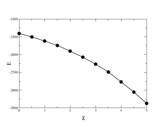
FIG. 6.: The energy dependence on $\chi$ calculated using Monte Carlo, $\xi=4.17$, $Z=201$, $n=160$ and $m=5$.

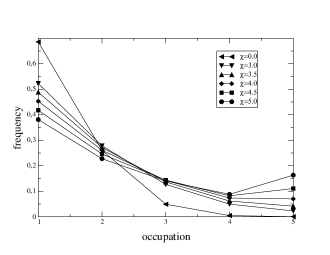
FIG. 7.: Histogram of cluster sizes for $Z$=201 and $n=160$, $\xi=4.17$.

V Conclusions

We have studied a simple model of micellization in the presence of polyelectrolyte. It is found that the mean field theory predicts a first order micellization transition for the ionic amphiphiles condensed on a polyion. This thermodynamic transition is an artifact of the mean field approximation and is the result of neglect of fluctuations associated with the short ranged hydrophobic interactions. Monte Carlo simulations show that the mean field works very well for small hydrophobicities, but fails completely for strong short ranged interactions. Indeed the simulations do not find any evidence of a phase transition. Nevertheless, if the hydrophobic interaction are sufficiently strong they will lead to significant correlations between the condensed amphiphiles, which can be interpreted as a micellar formation along the polyion chain.

ACKNOWLEDGMENTS

This work was supported in part by CNPq and Fapergs, Brazilian science agencies.

REFERENCES

- [1] T. Friedmann, Sci. Am. 276, 80 (1997).
- [2] M.J. Hope, B. Mui, S. Ansell, and Q. F. Ahkong, Mol. Membrane Biol. 15, 1 (1998).
- [3] P. L. Felgner, Sci. Am. 276, 86 (1997).
- [4] P. L. Felgner and G. M. Ringold, Nature 337, 387-388 (1989).
- [5] P. L. Felgner and G. Rhodes, Nature 349, 351 (1991).
- [6] I. M. Verma and N. Somia, Nature 389 239 (1997).
- [7] J. O. Rädler et al., Science 275, 810 (1997).
- [8] D. Harries et al., Biophys. J. 75, 159 (1998).
- [9] W. F. Anderson, Nature, 392, 25, (1998). Suppl.
- [10] K. Shirahama et al., Bull. Chem. Soc. Jpn. 60, 43 (1987).
- [11] A. V. Gorelov et al., Physica A249, 216 (1998).
- [12] H. Diamant and D. Andelman, Macromolecules 33, 8050 (2000).
- [13] H. Diamant and D. Andelman, Phys. Rev. E 61, 5296 (2000).
- [14] P. S. Kuhn, Y. Levin, and M. C. Barbosa, Chem. Phys. Lett. 298, 51 (1998).
- [15] P. S. Kuhn, Y. Levin, and M. C. Barbosa, Physica A266, 413, (1999).
- [16] P. S Kuhn, M. C. Barbosa, and Y. Levin, Physica A269, 278 (1999).
- [17] P. S Kuhn, M. C. Barbosa, and Y. Levin, Physica A274, 8 (1999).
- [18] P. S Kuhn, M. C. Barbosa, and Y. Levin, Physica A283, 113 (2000).
- [19] G. S. Manning, J. Chem. Phys. 51, 924 (1969).
- [20] Y. Levin, Europhys. Lett. 34, 405 (1996).
- [21] J. L. Barrat and J.F. Joanny, Adv. Chem. Phys. 94, 1 (1996).
- [22] P. Kuhn, Y. Levin, M.C. Barbosa, Macromolecules, 31, 8347 (1998)
- [23] J.J. Arenzon, Y. Levin, J.F. Stilck, Physica, A283, 1 (2000)