Dynamic structure factor of a superfluid Fermi gas

Abstract

We describe the excitation spectrum of a two-component neutral Fermi gas in the superfluid phase at finite temperature by deriving a suitable Random-Phase approximation with the technique of functional derivatives. The obtained spectrum for the homogeneous gas at small wavevectors contains the Bogoliubov-Anderson phonon and is essentially different from the spectrum predicted by the static Bogoliubov theory, which instead shows an unphysically large response. We adapt the results for the homogeneous system to obtain the dynamic structure factor of a harmonically confined superfluid and we identify in the spectrum a unique feature of the superfluid phase.

I Introduction

The techniques of atom trapping and cooling which have led to the realization of Bose-Einstein condensation in alkali gases are currently being employed to cool also the fermionic isotopes ⁴⁰K [1] and ⁶Li [2]. Dilute gases of fermionic atoms with attractive inter-particle interactions are predicted to undergo a superfluid transition at low temperatures ($T_{sup}\ll T_{F}$, where $T_{F}$ is the Fermi temperature). The simplest mechanism envisaged is a $s$-wave pairing [3, 4] which can be obtained, compatibly with the Pauli principle, between atoms belonging to two different internal states. The realization of a two-component Fermi gas in the superfluid state may provide a new physical system to study. Its properties are expected to be different from those of superfluid ³He, which has a $p$-wave pairing and is not in the dilute regime, and from conventional charged superconductors which have an excitation spectrum dominated by the Coulomb interaction [5] and only weakly modified by the superfluid transition.

An important issue for future experiments is to identify a clear signature of the superfluid transition in an atomic Fermi gas. Contrary to the case of atomic Bose-Einstein condensates, for fermions the superfluid transition affects only slightly the density profile and the internal energy of the gas [6]. A first idea is to measure the pair distribution function of the atoms, e.g. by using a laser probe beam [7]. A second idea is to look at the dynamical properties, which are expected to be dramatically modified by the transition. Several proposals have been put forward in this direction, such as Cooper-pair breaking via a Raman transition [8], measurement of the moment of inertia of the cloud [9], and excitation of collective modes in a harmonic trap by modulation of the trap frequencies [10] or rotation of the axis of the trap [11].

In this work we suggest to identify the superfluid phase through the measurement of the bulk excitations of the gas, i.e. excitations with a wavelength smaller than the spatial extension of the atomic cloud. This is complementary to the proposals in [10, 11] as it deals with high energy excitations in a quasi-homogeneous system at arbitrary temperature, and is not irrealistic from the experimental point of view, since efficient Bragg scattering techniques have already been successfully used to measure the excitation spectra of Bose condensates [12].

We obtain the excitation spectrum of the fluid in the dilute regime by employing the Random-Phase (or Time-Dependent Hartree-Fock-Gorkov) Approximation (RPA), which we derive explicitly for the two-component system of present interest by the technique of functional derivatives [13, 14]. We do not use here the usual static Bogolubov approximation [15] for two main reasons: (i) physically its excitation spectrum has a gap and therefore ignores the branch of phonon-like excitations (Bogolubov-Anderson phonon, [16, 17, 18]) expected on very general grounds to show up in homogeneous neutral superconductors with short range interactions [5], and (ii) the density-density response function obtained within this approximation shows an unphysically large response at small wavevectors and fails to satisfy the $f$-sum rule, which is a requirement deriving from the local particle conservation law.

We find that the RPA spectrum of a homogeneous two-component Fermi gas in the superfluid phase possesses the continuum of particle-hole excitations and a peak corresponding to the Bogoliubov-Anderson phonon; it satisfies the $f$-sum rule and includes naturally the Landau damping of the phonon due to the interplay with thermal excitations. We adapt the results obtained for the homogeneous system to describe harmonically confined gases by means of a local-density approximation, which predicts a broadening of the spectrum by taking into account the inhomogeneity of the density profile. We predict that the Bogoliubov-Anderson phonon, which is the main feature of the spectrum in the superfluid phase, would remain visible even in the trapped cloud.

The structure of this paper is as follows. In Sec. II we derive the density response function of the fluid in the RPA. In Sec. III we obtain the spectrum of density fluctuations first in the homogeneous case and then for an harmonically trapped gas. Finally, Sec. IV gives a summary of our results and offers some concluding remarks.

II Random-Phase Approximation

We describe a two-component atomic Fermi gas by the following Hamiltonian:

$$\hat{\cal H}-\mu\hat{\cal N} = \sum_{\alpha=\uparrow,\downarrow}\int d^{3}r\,\hat{\psi}^{{\dagger}}_{\alpha}({\mathbf{r}})\left(-\frac{\hbar^{2}}{2m}\nabla^{2}+V_{\mbox{ext},\alpha}({\mathbf{r}})+U({\mathbf{r}},t)-\mu_{\alpha}\right)\hat{\psi}_{\alpha}({\mathbf{r}})$$ (1)

$$+ \frac{1}{2}\sum_{\{\alpha,\beta\}=\uparrow,\downarrow}\int d^{3}r\int d^{3}{r^{\prime}}\,\hat{\psi}^{{\dagger}}_{\alpha}({\mathbf{r}})\hat{\psi}^{{\dagger}}_{\beta}({\mathbf{r}}^{\prime})v_{\alpha\beta}({\mathbf{r}}-{\mathbf{r}^{\prime}})\hat{\psi}_{\beta}({\mathbf{r}}^{\prime})\hat{\psi}_{\alpha}({\mathbf{r}})\;.$$ (2)

The fermionic field operators $\hat{\psi}_{\alpha}({\mathbf{r}})$ satisfy the usual anticommutation relations; the interactions are considered only in $s$-wave between fermions in different internal states and are modeled by the inter-particle potential $v_{\alpha\beta}({\mathbf{r}}_{1}-{\mathbf{r}}_{2})=\left(\begin{array}[]{cc}0&v_{\uparrow\downarrow}({\mathbf{r}}_{1}-{\mathbf{r}}_{2})\\ v_{\uparrow\downarrow}({\mathbf{r}}_{1}-{\mathbf{r}}_{2})&0\\ \end{array}\right)$, with $v_{\uparrow\downarrow}({\mathbf{r}}_{1}-{\mathbf{r}}_{2})=v_{\uparrow\downarrow}\delta({\mathbf{r}}_{1}-{\mathbf{r}}_{2})\partial_{r_{12}}(r_{12}\cdot)$. This model interaction potential, known as the Fermi pseudopotential, leads to a divergence-free BCS theory [19]. For the sake of generality we have included the presence of the external confinement via the trapping potentials $V_{\mbox{ext},\alpha}({\mathbf{r}})$ and the possibility of having different numbers of atoms in the two components; however in the following we shall restrict to the derivation of the equations in the homogeneous system and in the symmetric case $N_{\uparrow}=N_{\downarrow}=N/2$, which is the most favourable for the formation of Cooper pairs [4]. The effect of trapping potential present in a realistic experiment will be included later on with a local density approximation. The external perturbing field which is necessary to generate the total density response has been introduced as $U({\mathbf{r}},t)$. Physically $U$ represents the action of the probe applied in a real experiment; it may be a time-dependent perturbation applied to the magnetic trap [20], a probe laser beam [12] or a test particle [21]. Here we have assumed that the same potential $U$ acts in the same way on both components, and we shall determine the perturbation $\delta\rho({\mathbf{r}},t)$ on the total density induced by the probe potential $U({\mathbf{r}},t)$, assuming that the gas is initially at thermal equilibrium with a temperature $T$. We restrict to the linear response regime, where the density perturbation is a linear functional of the probe potential $U$ expressed through the density-density response function $\chi({\mathbf{r}}_{1},t_{1},{\mathbf{r}}_{2},t_{2})$, a function of two position vectors ${\mathbf{r}}_{1,2}$ and of two time variables $t_{1,2}$:

$$\delta\rho({\mathbf{r}}_{1},t_{1})=\int d^{3}r_{2}\,dt_{2}\ \chi({\mathbf{r}}_{1},t_{1},{\mathbf{r}}_{2},t_{2})U({\mathbf{r}}_{2},t_{2}).$$ (3)

In this section we explain how to calculate this response function in the Hartree-Fock-Gorkov approximation. We obtain general equations valid for an arbitrary trapping potential $V_{\mbox{ext}}({\mathbf{r}})$. We then solve these equations explicitly for a spatially homogeneous gas at thermal equilibrium, where $\chi$ is a function of ${\mathbf{r}}_{1}-{\mathbf{r}}_{2}$ and $t_{1}-t_{2}$ only.

To proceed with the derivation of the response function $\chi$, we follow the imaginary time Green’s function technique of the book of Kadanoff and Baym [13]. One first defines the two by two matrix of (normal and anomalous) Green’s functions in imaginary times

$$G(1,2)=\left(\begin{array}[]{cc}G_{\uparrow\uparrow}(1,2)&G_{\uparrow\downarrow}(1,2)\\ G_{\downarrow\uparrow}(1,2)&G_{\downarrow\downarrow}(1,2)\end{array}\right)\equiv-\langle{\rm T}\hat{\Psi}(1)\hat{\Psi}^{{\dagger}}(2)\rangle$$ (4)

where T is the time-ordering operator, $\hat{\Psi}(1)=\left(\begin{array}[]{c}\hat{\psi}_{\uparrow}(1)\\ \hat{\psi}_{\downarrow}^{{\dagger}}(1)\\ \end{array}\right)$, $\hat{\Psi}^{\dagger}(2)=\left(\hat{\psi}_{\uparrow}^{{\dagger}}(2),\hat{\psi}_{\downarrow}(2)\right)$, $\langle...\rangle$ indicates the average over the state of the system in the presence of the perturbing field $U$ and $(1,2)$ stands for $({\mathbf{r}}_{1},i\tau_{1},{\mathbf{r}}_{2},i\tau_{2})$, where $\tau_{1}$ and $\tau_{2}$ are real quantities. For more details on the imaginary time technique, we refer to reference [13]. We simply note that the various functions considered here can be obtained for real times by analytic continuation of their imaginary time values. From the equation of motion for the field operator in imaginary times one derives [13] the generalized Dyson equation for $G$:

$$G(1,2)=G_{0}(1,2)+\int d\bar{3}\int d\bar{4}\,G_{0}(1,\bar{3})\Sigma(\bar{3},\bar{4})G(\bar{4},2)+\int d\bar{3}\,G_{0}(1,\bar{3})W(\bar{3})G(\bar{3},2)\;,$$ (5)

where the $2\times 2$ matrix $G_{0}(1,2)$ is the solution of the equations of motion in absence of the interactions, $W(1)=\left(\begin{array}[]{cc}U(1)&0\\ 0&-U(1)\\ \end{array}\right)$ is the $2\times 2$ matrix of external field and $\Sigma(1,2)$ is the $2\times 2$ matrix of self-energies. Since we want to describe a dilute system, we work in the mean-field Hartree-Fock-Gorkov symmetry breaking approximation, where the self-energy reads

$$\Sigma_{HG}(1,2)=\delta(1,2)v_{\uparrow\downarrow}\left(\begin{array}[]{cc}\langle\hat{\psi}_{\downarrow}^{\dagger}(1)\hat{\psi}_{\downarrow}(1)\rangle&0\\ 0&-\langle\hat{\psi}_{\uparrow}^{\dagger}(1)\hat{\psi}_{\uparrow}(1)\rangle\end{array}\right)+v_{\uparrow\downarrow}(1,2)\left(\begin{array}[]{cc}0&G_{\uparrow\downarrow}(1,2)\\ G_{\downarrow\uparrow}(1,2)&0\end{array}\right).$$ (6)

Here we have used the notations $\delta(1,2)=\delta(\vec{r}_{1}-\vec{r}_{2})\delta(\tau_{1}-\tau_{2})/i$ and $v_{\uparrow\downarrow}(1,2)=v_{\uparrow\downarrow}({\mathbf{r}}_{1},{\mathbf{r}}_{2})\delta(\tau_{1}-\tau_{2})/i$. We remark that the Fock contribution is zero since the interaction takes place only between particles with opposite spins and $\langle\psi^{\dagger}_{\uparrow}\psi_{\downarrow}\rangle=0$ in the considered state of the system, hence the vanishing diagonal in the last term of Eq. (6).

Following a standard approach [13, 14], we then obtain the density response matrix in RPA by taking the functional derivative of the Green’s function with respect to the external field $U$: we define the generalized response matrix as the two by two matrix $L(1,2,3)=\sigma_{3}\delta G(1,2)/\delta U(3)$, where $\sigma_{3}$ is the third Pauli matrix $\left(\begin{array}[]{cc}1&0\\ 0&-1\\ \end{array}\right)$. The matrix giving the physical response is obtained from the limit $L(1,2)\equiv L(1,1^{+},2)$. The density-density response function $\chi$ is simply the trace over the two spin components of the response matrix:

$$\chi(1,2)=\mbox{Tr}\,L(1,2)=L_{\uparrow\uparrow}(1,2)+L_{\downarrow\downarrow}(1,2).$$ (7)

The equation for the density response in the Random-Phase Approximation is obtained by the functional derivative of the Dyson equation, Eq. (5), where the approximation (6) for the self energy has been employed. This yields:

$$L(1,2)=L^{0}(1,2)+\frac{v_{\uparrow\downarrow}}{2}\int d\bar{3}\,L^{0}(1,\bar{3})\chi(\bar{3},2)-\int d\bar{3}\int d\bar{4}\,\tilde{G}(1,\bar{3})M(\bar{3},\bar{4},2)\tilde{G}(\bar{4},1)v_{\uparrow\downarrow}(\bar{3},\bar{4})\;.$$ (8)

Here we have introduced the $2\times 2$ matrices $\tilde{G}(1,2)=\sigma_{3}G(1,2)$, $L^{0}(1,2)=\tilde{G}(1,2)\tilde{G}(2,1)$, and $M(1,2,3)=\left(\begin{array}[]{cc}0&L_{\uparrow\downarrow}(1,2,3)\\ L_{\downarrow\uparrow}(1,2,3)&0\end{array}\right)$. Physically $L^{0}(1,2)$ is the response matrix of the gas in the static Bogoliubov approximation, so that the reference system of the RPA is not the ideal gas but the Bogoliubov gas of quasiparticles.

It is possible to display the diagrammatic structure of Eq. (8) by separating out the “proper” part $\bar{L}(1,2)$ of the density response. We have therefore an equation which sums the bubble diagrams,

$$L(1,2)=\bar{L}(1,2)+\frac{1}{2}v_{\uparrow\downarrow}\int d\bar{3}\,\bar{L}(1,\bar{3})\chi(\bar{3},2)\;,$$ (9)

and an equation which defines the bubble as a sum of all the ladder diagrams,

$$\bar{L}(1,2)=L^{0}(1,2)-\int d\bar{3}\int d\bar{4}\,\tilde{G}(1,\bar{3})v_{\uparrow\downarrow}(\bar{3},\bar{4})\bar{M}(\bar{3},\bar{4},2)\tilde{G}(\bar{4},1)\;.$$ (10)

Here $\bar{M}=\left(\begin{array}[]{cc}0&\bar{L}_{\uparrow\downarrow}\\ \bar{L}_{\downarrow\uparrow}&0\end{array}\right)$.

We now specialize the previous equations to the case of a spatially homogeneous gas and to the dilute limit $\Delta\ll\epsilon_{F}$, where $\Delta$ is the gap and $\epsilon_{F}$ is the Fermi energy. All the response matrices depend then only on the relative spatial coordinates ${\mathbf{r}}={\mathbf{r}}_{1}-{\mathbf{r}}_{2}$ and the relative time coordinate $t=t_{1}-t_{2}$ and we introduce their double Fourier transforms with respect to $\mathbf{r}$ and $t$, e.g.

$$\bar{L}({\mathbf{q}},\omega)=\int d^{3}r\,dt\,\bar{L}({\mathbf{r}}_{1}={\mathbf{r}},t_{1}=t,{\mathbf{r}}_{2}={\mathbf{0}},t_{2}=0)\,e^{i({\mathbf{q}}\cdot{\mathbf{r}}-\omega t)}.$$ (11)

The following equation is obtained for $\bar{L}({\mathbf{q}},\omega)$ from the solution of Eq. (10) together with the regularization of the contact potential:

$$\bar{L}({\mathbf{q}},\omega)=A({\mathbf{q}},\omega)+v_{\uparrow\downarrow}\frac{4[C({\mathbf{q}},\omega)]^{2}}{1+v_{\uparrow\downarrow}B_{\mbox{reg}}({\mathbf{q}},\omega)}\;,$$ (12)

where $A({\mathbf{q}},\omega)$, $B_{\mbox{reg}}({\mathbf{q}},\omega)$ and $C({\mathbf{q}},\omega)$ are complex functions of the frequency to be evaluated numerically. We remark that the assumption $\Delta\ll\epsilon_{F}$ has considerably simplified the treatment by allowing to introduce only three basic functions ($A$, $B$ and $C$) in place of six required by the exact treatment [14]. The general expression $R({\mathbf{q}},\omega)$, where $R$ stands for $A$, $B$ or $C$ and $r$ stands for $a$, $b$, $c$, is given by [14]

$$R({\mathbf{q}},\omega)=\int\frac{d^{3}k}{(2\pi)^{3}}{r}_{L}({\mathbf{k}},{\mathbf{q}})(f(E_{+})-f(E_{-}))\left[\frac{1}{\hbar\omega+E_{+}-E_{-}+i\eta}-\alpha\frac{1}{\hbar\omega-(E_{+}-E_{-})+i\eta}\right]$$ (13)

$$+{r}_{B}({\mathbf{k}},{\mathbf{q}})(1-f(E_{+})-f(E_{-}))\left[\frac{1}{\hbar\omega-(E_{+}+E_{-})+i\eta}-\alpha\frac{1}{\hbar\omega+E_{+}+E_{-}+i\eta}\right]$$ (14)

where the “Landau” contributions ${r}_{L}({\mathbf{k}},{\mathbf{q}})$ are given by

$$a_{L}({\mathbf{k}},{\mathbf{q}}) = (1+(\xi_{+}\xi_{-}-\Delta^{2})/E_{+}E_{-})/4$$ (15)

$$b_{L}({\mathbf{k}},{\mathbf{q}}) = (1-(\xi_{+}\xi_{-}+\Delta^{2})/E_{+}E_{-})/4$$ (16)

$$c_{L}({\mathbf{k}},{\mathbf{q}}) = \Delta(1/E_{+}-1/E_{-})/8$$ (17)

and where the “Beliaev” contributions ${r}_{B}({\mathbf{k}},{\mathbf{q}})$ are given by

$$a_{B}({\mathbf{k}},{\mathbf{q}}) = (1-(\xi_{+}\xi_{-}-\Delta^{2})/E_{+}E_{-})/4$$ (18)

$$b_{B}({\mathbf{k}},{\mathbf{q}}) = (1+(\xi_{+}\xi_{-}+\Delta^{2})/E_{+}E_{-})/4$$ (19)

$$c_{B}({\mathbf{k}},{\mathbf{q}}) = -\Delta(1/E_{+}+1/E_{-})/8$$ (20)

for $A({\mathbf{q}},\omega)$, $B({\mathbf{q}},\omega)$ and $C({\mathbf{q}},\omega)$ respectively. The function $B({\mathbf{q}},\omega)$ as defined in Eq. (14) presents an ultraviolet divergence originating from the choice of a contact interaction potential. This divergence is removed in a systematic way by the use of the pseudopotential, which amounts here simply to subtracting the most diverging contribution in the form $1/(2\xi_{\mathbf{k}})$:

$$B_{\mbox{reg}}({\mathbf{q}},\omega)=B({\mathbf{q}},\omega)-\int\frac{d^{3}k}{(2\pi)^{3}}{\cal P}\left(\frac{1}{2\xi_{k}}\right)$$ (21)

where ${\cal P}$ represents the principal value [22]. We have used the notations $\xi_{\pm}=\hbar^{2}({\mathbf{k}}\pm{\mathbf{q}}/2)^{2}/2m+v_{\uparrow\downarrow}n/2-\mu$ where $n$ is the total equilibrium density of particles, $E_{\pm}=(\xi_{\pm}^{2}+\Delta^{2})^{1/2}$ and $f(E)=1/(\exp(\beta E)+1)$ is the Fermi distribution function at temperature $T$ with $\beta=1/(k_{B}T)$. The parameter $\alpha$ equals 1 for $A({\mathbf{q}},\omega)$ and $B({\mathbf{q}},\omega)$, while $\alpha$ equals $-$1 for $C({\mathbf{q}},\omega)$, and $\eta$ is a positive infinitesimal.

The final expression for the double Fourier transform of the density-density response function in RPA is obtained from Eq. (9) as:

$$\chi({\mathbf{q}},\omega)=\frac{2\bar{L}({\mathbf{q}},\omega)}{1-v_{\uparrow\downarrow}\bar{L}({\mathbf{q}},\omega)}\;.$$ (22)

This can be contrasted with the density-density response function in the static Bogoliubov approximation, which leads to $\chi({\mathbf{q}},\omega)=2A({\mathbf{q}},\omega)$ [23].

III The spectrum of density fluctuations

A Homogeneous system

Before displaying the fully numerical solution of Eqs. (12) and (22), we analyze some limiting cases. At temperatures higher than the BCS transition temperature we have $B({\mathbf{q}},\omega)=0$, $C({\mathbf{q}},\omega)=0$ and $A({\mathbf{q}},\omega)=\chi_{0}({\mathbf{q}},\omega)$, where $\chi_{0}({\mathbf{q}},\omega)$ is the well-known Lindhard function for the response of a ideal Fermi gas (see for example [24]). The RPA equation (12) reduces to the usual expression $\chi=2\chi_{0}/(1-v_{\uparrow\downarrow}\chi_{0})$, the factor two being due to the two spin components of the gas. In the case of repulsive interactions (i.e. $v_{\uparrow\downarrow}>0$) the equation shows a pole corresponding to the zero sound, while no well-defined collective excitation is stable in the case of attractive interactions.

At zero temperature, in the limit of small ${\mathbf{q}}$ and $\omega$ it is possible to estimate analytically the expression for the density response function; to lowest order in ${\mathbf{q}}$ we obtain

$$\chi({\mathbf{q}},\omega)=\frac{c_{B}^{2}q^{2}{\cal N}(\epsilon_{F})}{(\omega+i\eta)^{2}-c_{B}^{2}q^{2}(1+2k_{F}a_{\uparrow\downarrow}/\pi)},$$ (23)

where $c_{B}=v_{F}/\sqrt{3}$ is the sound velocity predicted by Bogoliubov, ${\cal N}(\epsilon_{F})=mk_{F}/\pi^{2}\hbar^{2}$ is the density of states at the Fermi level and $a_{\uparrow\downarrow}$ is the scattering length such that $v_{\uparrow\downarrow}=4\pi\hbar^{2}a_{\uparrow\downarrow}/m$. The pole yields a phonon-like excitation, corresponding to the Bogoliubov-Anderson sound for this system. Eq. (23) holds approximately until the phonon is stable, that is before it meets the continuum of quasiparticle-quasihole excitations, which has a threshold energy of $2\Delta$. Evidently the RPA expression is valid in the dilute limit $k_{F}|a_{\uparrow\downarrow}|\ll 1$.

It is easily checked that in the long-wavelenght limit the Bogoliubov-Anderson sound exhausts the $f$-sum rule $-\int d\omega\,\omega{\rm Im}\chi({\mathbf{q}},\omega)=\pi nq^{2}/m$, where $n$ is the total density of the gas. A more general proof can be obtained by noticing that the RPA, being equivalent to the time-dependent Hartree-Fock-Bogoliubov theory, automatically satisfies the continuity equation and hence the $f$-sum rule. On the contrary, the static Bogoliubov approximation results to be bad in the limit $q\rightarrow 0$: from Eq. (14) we estimate that $A(q\rightarrow 0,\omega)\propto\omega^{-3/2}$ in the high frequency limit, yielding an infinite contribution to the first moment integral.

We now turn to the presentation of numerical results. Rather than plotting the complex quantity $\chi({\mathbf{q}},\omega)$ we have chosen to represent the spectrum of total density fluctuations of wavevector ${\mathbf{q}}$, given by the dynamic structure factor $S({\mathbf{q}},\omega)$. On an experimental point of view the dynamic structure factor can be accessed via the rate of the scattering events of a probe particle by the gas leading to a momentum exchange $\hbar{\mathbf{q}}$ and to an energy exchange $\hbar\omega$ between the probe particle and the gas; on a theoretical point of view the dynamic structure factor of the gas is related to Im$\chi({\mathbf{q}},\omega)$ by the fluctuation-dissipation theorem [24]:

$$S({\mathbf{q}},\omega)=-(2\hbar/n)(1-\exp(-\beta\hbar\omega))^{-1}{\rm Im}\chi({\mathbf{q}},\omega).$$ (24)

Figure 1 shows the spectrum of a homogeneous superfluid at zero temperature as resulting from the full RPA calculation, compared to the predictions of the static Bogoliubov approximation: it is evident that for small $q$ ($\hbar q<2\Delta/c_{B}$) the Bogoliubov approximation yields an unphysically large response (Fig. 1 (a)). For larger $q$ the Bogoliubov-Anderson phonon falls in the continuum of quasi-particle quasi-hole excitations, and the two approximations yield almost the same result (Fig. 1 (b)), which is also close to the ideal-gas solution.

B Harmonically trapped system

We turn now to the situation where the particles are subject to an external harmonic confinement. We assume that the confining potential has the same action on both spin components, this is indeed the case in a laser induced trap. For simplicity we further assume that the resulting trapping potential is isotropic so that

$$V_{\mbox{ext},\uparrow}(r)=V_{\mbox{ext},\downarrow}(r)=\frac{1}{2}m\Omega^{2}r^{2}.$$ (25)

We consider bulk excitations of the harmonically confined cloud induced by a probe potential $U({\mathbf{r}},t)$ of wavevector ${\mathbf{q}}$ and frequency $\omega$. We characterize the density response of the gas by the dynamic structure factor calculated in the local-density approximation:

$$S_{LDA}({\mathbf{q}},\omega)=\frac{-2\hbar}{1-e^{-\beta\hbar\omega}}\int d^{3}r\,{\rm Im}\chi({\mathbf{q}},\omega;\mu(r),\Delta(r))\;,$$ (26)

where $\chi$ is the density response function derived in the previous section for the homogeneous system. This local-density approximation is valid for $q\geq 1/R$, where $R$ is the radius of the cloud, since it does not take into account surface modes [10] and in-gap single-particle excitations [26]. The same approach has already described successfully an experiment on trapped Bose-Einstein condensates, where the experiment has directly measured the function ${\rm Im}\chi({\mathbf{q}},\omega)\propto[S({\mathbf{q}},\omega)-S(-{\mathbf{q}},-\omega)]$ [12].

The position-dependent chemical potential and gap in Eq. (26) are defined as $\mu(r)=\mu-V_{\mbox{ext}}(r)$ and $\Delta(r)=\Delta[n(r)]$. The chemical potential $\mu$ of each spin component is determined by the normalization condition $N=\int d^{3}r\,n(r)$ where $N$ is the total number of particles in the gas. The equilibrium total density profile $n(r)$ and the gap $\Delta(r)$ are obtained first by numerical solution of the BCS equations in the homogeneous system

$$n=2\int\frac{d^{3}{k}}{(2\pi)^{3}}\left\{|u_{\bf k}|^{2}f(E_{\bf k})+|v_{\bf k}|^{2}[1-f(E_{\bf k})]\right\}\;,$$ (27)

$$\int\frac{d^{3}{k}}{(2\pi)^{3}}\left\{\frac{1-2f(E_{\bf k})}{2E_{\bf k}}-{\cal P}\left(\frac{1}{2\xi_{\bf k}}\right)\right\}=-\frac{1}{v_{\uparrow\downarrow}}\;,$$ (28)

and then by employing the Thomas-Fermi approximation (TFA) [27] to take into account the inhomogeneity due to the external confinement.

The main effect of the external confinement is a broadening of the spectrum, which is due to the inhomogeneous distribution of the density in the trap. This is illustrated already by a simple analytic expression for the dynamic structure factor at zero temperature in the low $q$ limit: integrating the imaginary part of Eq.(23) over space yields to lowest order in $k_{F}|a_{\uparrow\downarrow}|$

$$S_{LDA}^{\mbox{phonon}}({\mathbf{q}},\omega)=2\int d^{3}r\,A_{q}[n(r)]\delta(\omega-\omega_{q}[n(r)])=12\sqrt{3}\,\Omega^{-1}\left(\frac{\bar{\omega}}{\bar{q}}\right)^{3}\sqrt{2\bar{\mu}-3\left(\frac{\bar{\omega}}{\bar{q}}\right)^{2}}\;.$$ (29)

Here, $A_{q}[n]=mk_{F}c_{B}q/2\pi\hbar$, $\omega_{q}=c_{B}q$ and we have adopted the rescaled units $\bar{\omega}=\omega/\Omega$, $\bar{q}=\hbar q/\sqrt{m\hbar\Omega}$ and $\bar{\mu}=\mu/\hbar\Omega$. For the density profile we have taken the TFA expression $n(r)=(2m(\mu-V_{\mbox{ext}}(r))/\hbar^{2})^{3/2}/3\pi^{2}$, which neglects the Hartree mean field effect but turns out to be a good approximation in the dilute limit [4].

The numerical results at finite temperature and wavevector, presented in Fig. 2, show in the low temperature spectrum a peak corresponding to the Bogoliubov-Anderson phonon and include a high-frequency tail due to the contribution of multi-particle excitations. With increasing temperature, the asymmetric feature due to the Bogoliubov-Anderson phonon becomes less marked and disappears at $T\simeq\Delta/k_{B}$, when quasi-particle quasi-hole pairs are easily excited by thermal fluctuations.

IV Conclusion

In this paper, we have derived for a two-component spin-polarized Fermi gas a generalized Random-Phase Approximation to describe the excitation spectrum in the superfluid phase. We have shown that, contrary to the case of bosonic systems, the predictions of this theory – valid in the limit $k_{F}|a_{\uparrow\downarrow}|\ll 1$ – are essentially different from those of the “static” Bogoliubov theory, which instead yields an unphysically large signal at small wavevectors, due to the lack of local particle conservation.

The possible experiments that have motivated this theoretical work are light scattering [12] or scattering of test particles [28, 21] by a two-component Fermi gas stored in a dipole trap. The outcome of this type of experiments is described by the dynamic structure factor. We have therefore employed the results of the homogeneous system to predict in a local density approximation the dynamic structure factor of a harmonically trapped superfluid at finite temperature, and we have shown that the Bogoliubov-Anderson phonon – main feature of the superfluid phase in the spectrum of the homogeneous gas – would appear also in the response of the trapped system, as an asymmetric peak. We have investigated the effects of the temperature on the shape of the response, showing that the Bogoliubov-Anderson phonon should remain visible up to a temperature $T\simeq\Delta/k_{B}$. The observation of the Bogoliubov-Anderson phonon in the response of the gas to a probe beam may therefore provide a way to detect the presence of the superfluid phase in the experiments on alkali Fermi gases.

Our general RPA equations are also suitable for a full description of the inhomogeneous system without local density approximation, thus allowing in principle to take into account the discrete nature of the eigenmodes of the trapped gas. This would complete the static Bogoliubov treatment already performed in [19].

FIG. 1.: Dynamic structure factor of a homogeneous superfluid Fermi gas at $T=0$ for $q=0.054$ $k_{F}$ (a), and for $q=0.54$ $k_{F}$ (b), as predicted by the RPA (solid line) and by the static Bogoliubov approximation (dashed line). The results for a non-interacting Fermi gas (long-dashed line) are also shown. $k_{F}$ is the Fermi wavevector and $\epsilon_{F}=\hbar^{2}k_{F}^{2}/2m$ is the Fermi energy of the non-interacting Fermi gas at the same density. The parameters chosen are $\Delta=0.065\epsilon_{F}$ and $k_{F}a_{\uparrow\downarrow}=-0.04$.

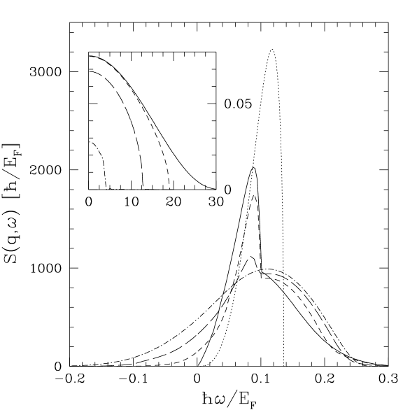
FIG. 2.: Dynamic structure factor of a confined superfluid Fermi gas for $\hbar q=4.15$ $p_{ho}$ at different temperatures: $T=0$ (solid line), $k_{B}T=0.014$ $E_{F}$ (short-dashed line), $k_{B}T=0.028$ $E_{F}$ (long-dashed line) and $k_{B}T=0.042$ $E_{F}$ (dot-dashed line). The critical temperature for the BCS transition is $k_{B}T=0.047$ $E_{F}$. The analytic expression for the broadening of the Bogoliubov-Anderson phonon in the low $q$ and zero temperature limit, Eq. (29), is given in dotted line. The inset shows the gap function in units of $E_{F}$ as a function of the radial coordinate $r/a_{ho}$, as obtained from the local-density approximation. The different line-styles correspond to the different temperatures of the main figure. $p_{ho}=\sqrt{\hbar m\Omega}$, $a_{ho}=\sqrt{\hbar/m\Omega}$ and $E_{F}$ is the Fermi energy of a harmonically trapped non-interacting Fermi gas with the same number of particles. The parameters used are $N=8\times 10^{7}$, $\Omega=2\pi\times 27.2$ s^-1 and $a_{\uparrow\downarrow}=-2160$ $a_{0}$ where $a_{0}$ is the Bohr radius.

- [1] B. DeMarco and D. S. Jin, Science 285, 1703 (1999).
- [2] M. O. Mewes, G. Ferrari, F. Schreck, A. Sinatra, and C. Salomon, Phys. Rev. A 61, 011403(R) (2000). See also cond-mat/0011291.
- [3] H. T. C. Stoof, M. Houbiers, C. A. Sackett, and R. G. Hulet, Phys. Rev. Lett. 76, 10 (1996).
- [4] M. Houbiers, R. Ferweda, H. T. C. Stoof, W. I. McAlexander, C. A. Sackett, and R. G. Hulet, Phys. Rev. A 56, 4864 (1997).
- [5] P. C. Martin, in Superconductivity, edited by R. D. Parks (Dekker, New York, 1969), Vol. 1.
- [6] In the dilute limit the superfluid transition almost does not affect the compressibility, because it modifies only slightly the Fermi sphere [15].
- [7] W. Zhang, C. A. Sackett and R. G. Hulet, Phys. Rev. A 60, 504 (1999); J. Ruostekoski, ibid. 61, 033605 (2000); F. Weig and W. Zwerger, Europhys. Lett. 49, 282 (2000).
- [8] P. Törma and P. Zoller, Phys. Rev. Lett. 85, 487 (2000).
- [9] M. Farine, P. Schuck and X. Viñas, Phys. Rev. A 62, 013608 (2000).
- [10] M. A. Baranov and D. S. Petrov, Phys. Rev. A 62, 041601(R) (2000).
- [11] A. Minguzzi and M. P. Tosi, Phys. Rev. A 63, 023609 (2001).
- [12] D. M. Stamper-Kurn, A. P. Chikkatur, A. Görlitz, S. Inouye, S. Gupta, D. E. Pritchard and W. Ketterle, Phys. Rev. Lett. 83, 2876, (1999).
- [13] L. P. Kadanoff and G. Baym, Quantum Statistical Mechanics (W. A. Benjiamin, New York, 1962).
- [14] R. Côté and A. Griffin, Phys. Rev. B 48, 10404 (1993).
- [15] P. de Gennes, Superconductivity of Metals and Alloys (Addison-Wesley, New York, 1966).
- [16] N. N. Bogoliubov, V. V. Tolmachev, and D. V. Shirkov, New Method in the Theory of Superconductivity (Academy of the Sciences of the U.S.S.R., Moscow, 1958).
- [17] P. W. Anderson, Phys. Rev. 112, 1900 (1958).
- [18] A. J. Leggett, Phys. Rev. 140, 1869 (1965).
- [19] G. Bruun, Y. Castin, R. Dum and K. Burnett, Eur. Phys. J. D 7, 433 (1999)
- [20] D. S. Jin, J. R. Ensher, M. R. Matthews, C. E. Wieman and E. A. Cornell, Phys. Rev. Lett. 77, 420 (1996); M.-O. Mewes, M. R. Andrews, N. J. van Druten, D. M. Kurn, D. S. Durfee, C. G. Townsend and W. Ketterle, Phys. Rev. Lett. 77, 988 (1996).
- [21] A. P. Chikkatur, A. Görlitz, D. M. Stamper-Kurn, S. Inouye, S. Gupta, and W. Ketterle, Phys. Rev. Lett. 85, 483 (2000).
- [22] In the limit , this leads to . By using the gap equation (28) one obtains .
- [23] see for example A. L. Fetter and J. D. Walecka, Quantum Theory of Many-Particle Systems (McGrawHill, New York, 1971).
- [24] D. Pines and P. Nozières, The Theory of Quantum Liquids (Benjamin, New York, 1966), Vol. 1.
- [25] P. Nozières and D. Pines, The Theory of Quantum Liquids. Volume II, Superfluid Bose Liquids (Addison-Wesley, Redwood City (CA), 1990).
- [26] M. A. Baranov, JETP Lett. 70, 396 (1999).
- [27] The TFA amounts to determining the density profile from the knowledge of the density dependence of the chemical potential in the homogeneous system , i.e. by inverting numerically the function .
- [28] G. Ferrari, Phys. Rev. A 59, R4125 (1999).