Anomalous Roughness, Localization, and Globally Constrained Random Walks

Abstract

The scaling properties of a random walker subject to the global constraint that it needs to visit each site an even number of times are determined. Such walks are realized in the equilibrium state of one dimensional surfaces that are subject to dissociative dimer-type surface dynamics. Moreover, they can be mapped onto unconstrained random walks on a random surface, and the latter corresponds to a non-Hermitian random free fermion model which describes electron localization near a band edge. We show analytically that the dynamic exponent of this random walk is $z=d+2$ in spatial dimension $d$. This explains the anomalous roughness, with exponent $\alpha=1/3$, in one dimensional equilibrium surfaces with dissociative dimer-type dynamics.

I introduction

Random walks provide the key to the scaling properties of many physical phenomena. Some examples are: surface diffusion, wave packet spreading in quantum mechanics, equilibrium commensurate-incommensurate phase transitions in physisorbed monolayers on substrates, and one dimensional (1D) interfaces in equilibrium and in stationary growing states [2, 3, 4]. In its elementary formulation, a particle moves through $d$ dimensional space by jumping during each discrete time step over a displacement vector $\vec{x}$, according to a given (localized) probability distribution $W(\vec{x})$. The fluctuations in the position, ${\vec{n}}_{t}=\sum_{t^{\prime}=1}^{t}{\vec{x}}_{t^{\prime}}$, after $t$ time steps, obey the scaling form

$$\Delta{\vec{n}}_{t}\equiv\langle|{\vec{n}}_{t}-\langle{\vec{n}}_{t}\rangle|^{2}\rangle^{1/2}\sim t^{1/z}$$ (1)

and the spatial probability distribution $P(\vec{n},t)$ develops at large time scales into the Gaussian form

$$P({\vec{n}},t)=\frac{1}{(4\pi Dt)^{d/z}}\exp\left[-{|{\vec{n}}|^{2}}/{4Dt^{2/z}}\right]~{},$$ (2)

which is invariant under the scale transformation $P\to b^{d}P$, $t\to b^{z}t$ and $\vec{n}\to b\vec{n}$. $z$ is the so-called dynamic exponent, and has the simple value $z=z_{rw}=2$ in all dimensions, as is obvious from the linear character of the underlying diffusion equation. Scale invariance is generic to many other dynamic processes as well, but with typically non-trivial values for $z$. Kardar-Parisi-Zhang (KPZ) type surface growth [5], and statistical population dynamics like directed percolation and directed Ising type processes are examples of this [6]. In such processes random walk (diffusion) arguments still play a central role, e.g., $z_{rw}$ typically appears within molecular field type approximations.

The scaling properties of stochastic processes can be classified in so-called universality classes, according to the symmetries and conservation laws of the underlying dynamic rules. In analogy with equilibrium critical phenomena, dynamic critical exponents are universal quantities, that are insensitive to varying details of the dynamic rule. For example, all random walks have $z=z_{rw}=2$, irrespective of the shape of the displacement distribution $W(\vec{x})$. To break out of the $z_{rw}$ straight jacket, something more drastic has to change. Examples of anomalous diffusion are: Levi flights, where the typical length of the displacement is divergent; correlated random walks, where the steps have long range temporal correlations [3]; walks in a quenched randomness environment, like polymers in disordered media [7, 8]; and also diffusion on a one dimensional lattice, where the particles can move only in dimer form  [9]. The latter leads to an infinite number of conserved quantities, and density auto-correlation functions that decay as power-laws with anomalous exponents.

In this paper, we investigate the scaling properties of so-called even-visiting random walks (EVRW) on a $d$ dimensional hypercubic lattice. During each time step $(0\leq t^{\prime}<t)$ the random walker hops to one of its nearest neighbor sites with equal probability. However, unlike normal random walks, it is required to visit every site an even number of times before the walk terminates at time $t$. This gives rise to anomalous scaling. The even-visiting condition imposes a (mod 2 type) global constraint on the motion of the random walker, which it can satisfy only through correlated movements. The origin and nature of this type of anomalous scaling is completely different from those in the examples mentioned above.

This study of EVRW’s is complementary to our recent work on dissociative dimer-type surface growth in one dimension (1D) [10]. The surface grows and erodes by the deposition and evaporation of dimers only. Those dimers dissociate while on the surface (but do not diffuse) such that each monomer can arrive and depart with a different partner. This growth rule implies that the number of particles at each height level is globally (but not locally) conserved mod $2$. Compared to conventional (monomer deposition type) surface roughness, it imposes a global constraint on the fluctuations of the surface and leads to anomalous equilibrium roughness. The mod 2 conservation of the particle number in dimer growth is equivalent to the even-visiting constraint in random walks, and the anomalous surface roughness is linked to the anomalous scaling of the EVRW.

There exists a second completely different type of application of EVRW’s. The time evolution operator of the random walk can be cast in the form of quantum mechanical non-interacting electrons moving in a random medium. The global EVRW constraint translates into spatial and directional randomness of the hopping amplitudes and a non-Hermitian random Hamiltonian (Sec. IV D). The spectral properties of such Hamiltonians are a topic of growing research, in particular their localization-delocalization transition aspects [11, 12]. Our EVRW scaling involves only one electron and therefore relates to the scaling of the electron eigenstates near the bottom of the (almost empty) energy band. Those edge states have so-called Lifshitz tails, with essential singularities in the disorder-averaged density of states [13]. Our study of EVRW’s elucidates the nature of the edge states.

The EVRW problem naturally generalizes to Q-visiting random walks (QVRW) with a constraint that the number of visits to each site must be multiple of Q. Diffusive motion of the QVRW describes the stationary state roughness of dissociative Q-mer growth, where a surface grows (erodes) by the deposition (evaporation) of a Q-mer. This conserves the number of particles at each height level modulo Q, which corresponds to the Q-visiting constraint. In our discussion we will focus mostly on EVRW and dissociative dimer type growth, but most results are easily extended to QVRW and the scaling properties turn out to be independent of Q.

This paper is organized as follows. In Sec. II, we review one dimensional dissociative dimer type dynamics [10], and present additional numerical results showing the anomalous roughness of the equilibrium surface.

In Sec. III, we map this dimer growth model onto the 1D EVRW and present numerical results for the anomalous diffusion in 1D EVRW’s. The finite size scaling type exact enumeration and Monte Carlo simulation results suggest that the dynamic exponent of the 1D EVRW is equal to $z\simeq 3.0$. We also devise an analytic scaling argument, a healing time argument, that predicts that the dynamic exponent is equal to $z=d+2$ in $d$ dimensions. The healing time argument presumes the existence of a crossover time scale $\tau_{\text{free}}\sim t^{2/(d+2)}$, within which the random walker is not influenced by the global even-visiting constraint imposed at time $t$. We numerically confirm that such a time scale is present in $d=1$ and $d=2$.

In Sec. IV, we embed the EVRW into an Ising spin environment. A $S_{\vec{n}}=\pm 1$ spin is assigned to every site. Each of them points up at time $t=0$. Next, the particle moves as in a conventional unconstrained random walk, but the Ising spin at site $\vec{n}$ flips with probability $e$ (or not with probability $f=1-e$) each time the particle visits that site. The global EVRW constraint can now be represented by the requirement that all spins must be pointing up again at time $t$, i.e., by projecting out from all conventional RW configurations those that leave spins pointing down. The even-visiting walks condition obviously requires that $e=1$, but it is advantageous to proceed with generalized values $0\leq e\leq 1$. We call this generalized version the stochastic even-visiting random walk (SEVRW). Next, we construct the time evolution operator of the Ising spins and the random walker. The spin part is easily diagonalized and the result has the form of a non-Hermitian single particle quantum Hamiltonian with quenched randomness. The latter can also be interpreted as the transfer matrix (thermal equilibrium) of a polymer fluctuating in an environment with randomly placed defect-lines.

In Sec. V we focus on one special point in the SEVRW model, $e=f=1/2$. There the 1D model is easily soluble. The dynamic exponent is exactly equal to $z=3$. This point plays the role of stable fixed point in the sense of renormalization transformations in the EVRW phase diagram. The EVRW, although at the border, belongs to its basin of attraction.

In Sec. VI we discuss the same issues as in Sec. V, but now in the framework of the non-Hermitian quantum Hamiltonian. The anomalous dynamic exponent $z=d+2$ relates to so-called Lifshitz tails in the density of states near the edge of the energy band. We conclude with a brief summary and discussion, in Sec. VII.

II Dissociative Dimer Surface Dynamics

A surface roughness

Equilibrium and non-equilibrium properties of 1D interfaces like crystal surfaces have attracted considerable interest [14]. Interfaces display intriguing scaling properties and their growth dynamics is well understood in terms of a few universality classes. KPZ growth is one of the examples [5]. An interesting quantity associated with interface roughness is the averaged width, $W$, i.e., the standard deviation of the interface height $h_{l}(t)$ ($l=1,\ldots,L$):

$$W(L,t)^{2}=\left\langle\frac{1}{L}\sum_{l=1}^{L}h_{l}(t)^{2}-\left(\frac{1}{L}\sum_{l=1}^{L}h_{l}(t)\right)^{2}\right\rangle\ ,$$ (3)

where $L$ is the substrate size. The width satisfies the dynamic scaling relation

$$W(L,t)=L^{\alpha}f(t/L^{z_{W}})\ ,$$ (4)

where the scaling function $f(x)$ behaves as

$$f(x)\sim\left\{\begin{array}[]{c}x^{\beta}\quad\mbox{for}\quad x\ll 1\\ \mbox{const.}\quad\mbox{for}\quad x\gg 1\ .\end{array}\right.$$ (5)

The stationary state roughness exponent $\alpha$ and dynamic exponent $z_{W}=\alpha/\beta$ are universal quantities.

In most growth models the structural properties of the depositing (evaporating) particles are explicitly or implicitly presumed to be geometrically featureless monomers. Nevertheless, the geometric features of the particle shapes can strongly affect the growth dynamics and the stationary state scaling properties [10].

B dimer dynamics

Consider a crystal built from atoms of type $X$. Assume that deposition and evaporation takes place in contact with a gas where the atoms only appear in molecular dimer form $X_{2}$, and assume that such dimers can only land and depart from the interface when aligned with the surface. Upon deposition a dimer attaches to two nearest neighbor surface sites and loses its dimer character. Upon evaporation, two nearest neighbor surface atoms form a dimer and depart from the crystal. This dissociative character of the dimers is the essential feature leading to the anomalous surface roughness in the equilibrium state.

We describe the 1D surface configurations in terms of integer height variables subject to the so-called restricted solid-on-solid (RSOS) constraint, $h_{l}-h_{l+1}=0,\pm 1$. The dynamic rule is as follows. First, select at random a bond $(l,l+1)$. If the two sites are not at the same height, no evaporation nor deposition takes place. If the two sites are at the same height, deposition of a dimer covering both sites is attempted with probability $p$, or evaporation of a dimer with probability $q=1-p$ (see Fig. 1). Processes are rejected if they would result in a violation of the RSOS constraint.

Surfaces growing according to such dissociative dimer dynamic rules behave fundamentally different from those following monomer-type growth rules. The latter, irrespective of being in equilibrium or in a stationary growing state, display, with only a few very notable exceptions, the universal roughness exponent $\alpha=1/2$; as exemplified in the Edwards-Wilkinson (EW) [15] and the KPZ [5] universality classes. The universal value of $\alpha$ is understood from a random walk argument. To be precise, a 1D surface can be mapped on the time trajectory of a particle in 1D by identifying the height $h_{l}$ at each site $l$ with the particle position $n_{t}$ at time $t=l$. The steps in 1D surfaces are uncorrelated beyond a definite correlation length. Therefore the particle performs a random walk with displacement fluctuations $|n_{t}-n_{t^{\prime}}|\sim(t-t^{\prime})^{1/z_{rw}}$ at large time scales. This yields the value of the stationary state roughness exponent $\alpha=1/z_{rw}=1/2$.

Dissociating dimer growth circumvents the random walk argument by means of a novel type of non-local topological constraint. The dimer aspect requires that the number of particles at every surface height level must be conserved modulo 2. The dissociative character of the dimers transforms this into a non-local global feature. This leads to various interesting phenomena. In equilibrium, the surface is rough but with anomalous scaling exponents [10, 16]. Out of equilibrium, while growing or evaporating, it always facets [10]. Moreover, when the model is extended by introducing a so-called reduced digging probability at flat segments, towards a directed Ising type roughening transition in the extreme no-digging limit, the roughness becomes even more complex [10, 17]. The non-equilibrium faceting aspects are already well documented in Ref. [10]. Here we focus on the anomalous equilibrium roughness.

C anomalous equilibrium roughness

At $p=q$ the above dynamic rule satisfies the detailed balance condition and the stationary state distribution is a genuine Gibbs type equilibrium state. We study the dynamic scaling of the surface width via Monte Carlo (MC) simulations. The crystal size $L$ is even, with periodic boundary conditions, $h_{L+l}=h_{l}$, and we use as initial condition a flat surface, $h_{l}=0$ for all $l$. The surface width is measured and averaged over $N_{s}$ independent MC runs, ranging from $N_{s}=5000$ for $L=2^{5}$ to $N_{s}=500$ for $L=2^{10}$.

The results are shown in Figs. 2 (a) and (b). The surface width does not obey monomer growth type EW scaling with $\alpha=1/2$ and $\beta=1/4$. The dimer surface width saturates slower $(\beta<1/4)$ and is definitely less rough in equilibrium ($\alpha<1/2$). Notice the large corrections to finite size scaling of the width in both the temporal and spatial domains. These prevent us from obtaining accurate values for the exponents $\alpha$ and $\beta$ from simple log-log type plots of the width versus $t$ and $L$. Instead, we define effective exponents

$$\alpha(L)\equiv\ln[W(mL,\infty)/W(L,\infty)]/\ln m$$ (6)

and

$$\beta(t)\equiv\ln[W(L,mt)/W(L,t)]/\ln m\ ,$$ (7)

where $m$ is arbitrary (we choose $m=2$) and $W(L,\infty)$ denotes the saturated width. For $\alpha(L)$, we use data for $L=2^{5},\ldots,2^{10}$, and for $\beta(t)$, the data at $L=2^{13}$ at times shorter than $t<10^{5}$ where finite size effects are still invisible. The results are shown in Figs. 2 (c) and (d). We estimate

$$\alpha=0.29(4),\quad\beta=0.111(2)\ .$$ (8)

and $z_{W}\simeq 2.6(5)$, since $z_{W}=\alpha/\beta$. The exponents are definitely different from those of ordinary equilibrium rough interfaces but the precise values remain uncertain.

The mod 2 non-local conservation of particle number is clearly the most promising candidate for being the origin of the anomalous scaling behavior; as confirmed in the following sections. However there exist additional more local conserved quantities in the dimer dynamics. When a dimer desorbs or adsorbs, the surface heights at two nearest neighbor sites change by one unit simultaneously. This implies conservation of the anti-Bragg, $k=\pi$, Fourier component of the surface height

$$\tilde{h}_{k}\equiv\frac{1}{\sqrt{L}}\sum_{l=1}^{L}e^{-ikl}h_{l}\ .$$ (9)

In other words, the dynamics is not ergodic; surface configurations with different values of $\tilde{h}_{k=\pi}$ are dynamically disconnected. Therefore the scaling properties may depend on the initial condition. Such types of effects are studied in Ref. [16] in the context of dissociative $k$-mer growth in body-centered solid-on-solid type models, $h_{l}-h_{l+1}=\pm 1$.

D surface diffusion

In our model the particles do not diffuse along the surface. In actual experimental settings, surface diffusion cannot be ignored. The $k=\pi$ broken ergodicity is restored by diffusion, but the mod 2 conservation is preserved as long as diffusion across steps is forbidden. Such jumps to higher and lower levels are suppressed by so-called Schwoebel barriers [18]. This means that the anomalous surface roughness discussed here can be observed at time scales smaller than the characteristic time associated with jumps across steps, provided the other time scales are short (high surface deposition rates).

To test the robustness of anomalous dimer roughness and to verify the essential role of the global mod 2 particle conservation at each height level, we add to the dimer growth model diffusion of surface atoms within terraces. The surface is again described by integer height variables $h_{l}$, subject to the RSOS constraint and periodic boundary conditions. The dynamic rule is as follows. Select at random a bond $(l,l+1)$, and attempt with equal probability: a dimer deposition or evaporation just like above; or a monomer jump from site $l$ to one of its nearest neighbor sites. The move is rejected if it would result in a violation of the RSOS constraint. Since the RSOS condition is imposed at every stage, jumps across steps are automatically forbidden.

Starting from a flat surface at $t=0$, the surface widths are measured for $L=2^{5},\ldots,2^{9}$. The results are shown in Fig. 3(a). They are qualitatively the same as in the absence of diffusion. The exponents $\alpha$ and $\beta$ are determined in the same way as in Eqs. (6) and (7), see Fig. 3 (b) :

$$\alpha=0.31(3),\quad\beta=0.115(5)\ .$$ (10)

The finite size corrections to scaling are again very large. The exponents are slightly larger than in Eq. (8), but, within the current numerical accuracy we cannot distinguish one from the other.

We conclude that dissociative dimer equilibrium dynamics represents a new universality class for interface roughness. Surface diffusion within terraces is irrelevant and this new universality class is characterized by the topological constraint caused by the mod 2 conservation of the number of particles at every height level.

III Even-visiting random walks

A the model

The above numerical study of dissociative dimer type dynamics clearly indicates that the equilibrium scaling properties of the interface belong to a different universality class than conventional monomer type dynamics. We also identified the most likely origin of this: the constraint that the number of particles at each height level must be preserved modulo 2 in a global non-local manner. The exact value of the exponent $\alpha$ is difficult to pin point from the MC results, due to strong corrections to scaling. To resolve this, we investigate in this section the properties of a random walk with the constraint that it needs to visit every site an even number of times before it terminates. This is the so-called even-visiting random walk (EVRW).

Consider a random walker on a 1D lattice, which is required to jump during each time step one site to the left or the right with equal probability, $n_{t^{\prime}+1}=n_{t^{\prime}}\pm 1$. $n_{t^{\prime}}$ denotes the position of the walker at time $t^{\prime}$. The walker is demanded to visit every site $n$ an even number of times after $t$ time steps.

We focus our presentation on the EVRW in one dimension. The generalization to $d>1$ is straightforward and mentioned when appropriate. Moreover, it is natural to expand the EVRW into a Q-visiting random walk (QVRW) with the constraint that each site must be visited a multiple of Q-times. We obtained numerical results for $Q\geq 3$, but since we did not detect any differences from the scaling behaviors at $Q=2$ [19], we limit this presentation to EVRW.

The connection with dimer surface dynamics is self-evident. The probability distribution of EVRW represents the equilibrium Gibbs distribution, i.e., the equilibrium state of a surface where all configurations that satisfy the mod 2 constraint are equally likely. There is one minor difference between our RSOS dimer model and the above EVRW. In the latter the particle is required to make a hop during every time step, $\Delta n=\pm 1$, while in the RSOS dimer dynamics it is allowed to stay at the same site, $\Delta n=0,\pm 1$. Figure 4 shows examples of both. This so-called body-centered solid-on-solid version of the EVRW is more compact and converges numerically faster.

B exact enumerations

The number of possible space-time configurations of a normal 1D random walker is equal to $Z_{RW}(t)=2^{t}$. The even-visiting constraint excludes most of those walks. It is of interest to know whether the total number of EVRW’s still scales exponentially as $Z(t)\sim\mu^{t}$, and if so, whether $\mu$ remains equal to $2$. For that purpose, we enumerate all EVRW’s that start and return to the origin ($n=0$) after $t$ time steps, using the exact (but not closed form) expressions, Eqs.(11) and (12) below, which were developed in Ref. [20] in the following manner.

Denote the number of steps to the right (left) from site $n$ to $n+1$ ($n-1$) by $r_{n}$ ($l_{n}$). The number of visits of site $n$ is equal to $v_{n}=r_{n}+l_{n}$ and the sum of all visits is equal to total number of time steps $t=\sum_{n}v_{n}$. The return-to-origin condition implies that $r_{n}=l_{n+1}$, i.e., that $v_{n}=r_{n}+r_{n-1}=l_{n+1}+l_{n}$, and that $l_{n}$ and $r_{n}$ must be even for all $n$, such that $t=\sum_{n}v_{n}=2\sum_{n}r_{n}$ is a multiple of $4$ instead of $2$.

Every walk can be specified by the left boundary of the walk $n_{\min}$, and $m$ positive integer variables $[s_{1},\ldots,s_{m}]$. The excursion $m$ is defined by the distance between the right and left boundaries of the walk. The number of steps from site $n$ to $n+1$ is equal to $r_{n}=2s_{n-n_{\min}+1}$ with the understanding that $s_{n^{\prime}}=0$ for $n^{\prime}\leq 0$ and $n^{\prime}>m$. The number of walks with the same set of positive integers $[s_{1},\ldots,s_{m}]$ can be readily evaluated and is equal to  [20]

$$S_{[s_{1},\ldots,s_{m}]}=\frac{t}{2s_{1}}\prod_{i=1}^{m-1}\frac{(2s_{i}+2s_{i+1}-1)!}{(2s_{i+1})!(2s_{i}-1)!}$$ (11)

for $m\geq 2$ and is equal to $S_{[s_{1}]}=2$ for $m=1$. The total number of the EVRW’s is given by the sum

$$Z^{0}(t)=\sum_{m=1}^{t/4}\sum_{\{s_{i}\}}^{\prime}S_{[s_{1},\ldots,s_{m}]}\ ,$$ (12)

where the prime in the second summation denotes the constraint that $t=4\sum_{i}s_{i}$, and the superscript in $Z^{0}$ represents the return-to-origin condition.

Although analytically exact, this formula still involves infinite sums. Therefore we must resort to numerical enumerations to determine the scaling properties. This has to be a finite size scaling type analysis because of the numerical upper limit for $t$.

In Fig. 5(a), we plot $Z^{0}(t)$ as function of time for $t\leq 140$. The linear dependence in this semi-log plot indicates an exponential form $Z^{0}(t)\sim\mu^{t}$. Next, we define an effective finite size exponent as

$$\mu(t)=[Z^{0}(t)/Z^{0}(t-4)]^{1/4}.$$ (13)

The corrections to scaling in Fig. 5(b) are strong, but a Neville type extrapolation analysis [21] yields

$$\mu=2.000(2)\ .$$ (14)

Despite the severe global constraint, the total number of EVRW’s scales asymptotically in the same way as that of normal random walks with $\mu=2$.

Figs. 5(a) and (b) indicate the presence of strong corrections to scaling. They are of an exponential form

$$Z^{0}(t)\sim 2^{t}e^{-at^{\theta}}\ .$$ (15)

as shown in Fig. 5(c). The slope yields

$$\theta=0.34(2).$$ (16)

In Sec. V, we will argue that the exponent $\theta$ is a universal quantity, and equal to the inverse of the dynamic exponent $z$ of the EVRW; $\theta=1/z$.

We also performed an exact enumeration of the finite size scaling of the width of the EVRW. All configurations counted in Eq. (11) have the same number of visits $v_{n}$ up to a constant shift in $n$. Hence, they all have the same width, $W[\{s_{i}\}]=(\bar{n^{2}}-\bar{n}^{2})^{1/2}$, with

$$\bar{n} = \frac{2}{L}\sum_{i=1}^{m}(2i+1)s_{i}$$

$$\bar{n^{2}} = \frac{2}{L}\sum_{i=1}^{m}(i^{2}+(i+1)^{2})s_{i}\ .$$

The ensemble averaged surface width

$$W^{2}=\frac{1}{Z^{0}(t=L)}\sum_{m=1}^{t/4}\sum_{\{s_{i}\}}^{\prime}W[\{s_{i}\}]^{2}S_{[s_{1},\ldots,s_{m}]}$$ (17)

is evaluated numerically and plotted in Fig. 6(a). The roughness exponent $\alpha$, $W\sim L^{\alpha}$, is estimated from an effective exponent

$$\alpha(L)=\frac{L}{4}\left(\frac{W(L)}{W(L-4)}-1\right)\ ,$$ (18)

see Fig. 6(b). Again, the convergence is slow, but the Neville type extrapolation yields

$$\alpha=0.327(9)\ .$$ (19)

Within the numerical accuracy, this result is consistent with those in the two dimer growth models (with/without monomer diffusion) of the previous section, see Eqs. (8) and (10).

The surface roughness exponent $\alpha$ is simply related to the dynamic exponent $z$ of the EVRW as $z=1/\alpha$. So the above numerical result implies that

$$z=3.06(8)\ .$$ (20)

All the results of this section are checked numerically for $Q=3,4,5$ in the QVRW model. We find no Q-dependence of the values of scaling exponents [19].

C Gaussian distributions

We performed Monte Carlo simulations to determine the probability distribution $P(n,t)$ for the EVRW, i.e., the probability to start at site $n=0$ and end after time $t$ at site $n$. This was done by brute force. We simply generated an ensemble of normal random walks and trashed the ones that did not satisfy the EVRW condition. The ratio decreases rapidly. For example, out of a total of $2\times 10^{9}$ normal random walks only about $600$ walks satisfy the constraint at $t=500$.

The distribution function is shown in Fig. 7(a) and can be assumed to obey the scaling form

$$P(n,t)=\frac{1}{t^{1/z}}{\cal F}(n/t^{1/z})$$ (21)

with $z$ the dynamic exponent. The best data collapse is obtained for $1/z=0.32$, as shown in Fig. 8. This value of $z$ is consistent with the exact enumeration results of the previous subsection. It is also consistent with a direct evaluation of the second moment of the distribution function data, which yields that

$$\Delta n=\left[\sum_{n}n^{2}P(n,t)-\left(\sum_{n}nP(n,t)\right)^{2}\right]^{1/2}\$$ (22)

scales as $\Delta n\sim t^{1/z}$, with $z\simeq 3.3$ as shown in Fig. 7(b).

The functional form of the scaling function ${\cal F}$ is a surprise. It is of the form of ${\cal F}(u)=Ae^{-B|u|^{\Delta}}$ , as shown in Fig. 8, with $\Delta\simeq 1.98$. This means that the probability distribution is Gaussian in nature,

$$P(n,t)=At^{-1/z}\exp\left[-B\left(n/t^{1/z}\right)^{2}\right]\ .$$ (23)

This is surprising, because in other models with anomalous surface roughness, such as Levi flights, the probability distribution is certainly not Gaussian [3].

Gaussian distributions with $z=2$ are characteristic for uncorrelated random processes. The appearance of a Gaussian shaped scaling function in the EVRW problem suggests us to search for an effective representation of the EVRW in which the correlation effects somehow transform away, with the possibility for an exact derivation of the EVRW dynamic exponent, possibly $z=3$. This is the topic of the next section.

IV Random Walks Coupled to Ising Spins

A defect spreading

The even-visiting constraint is non-local in time. To keep track of this constraint in a local way, we can add an Ising field to a normal conventional random walk, i.e., a marker $S_{n}=\pm 1$ to each site, that keeps track of the visits in the past. Initially at time $t^{\prime}=0$, all spins are prepared in the spin-up state. $S_{n}$ flips each time the random walker visits site $n$. The requirement that all spins are pointing up at $t^{\prime}=t$, represents the EVRW constraint. The generalized distribution ${\cal P}(\{S\};n)_{t}$ contains all the information we need. $n$ is the location of the random walker at time $t$ and $\{S\}$ the spin configuration. ${\cal P}(\{+\};n)_{t}$ is the EVRW distribution.

Each down spin at intermediate time $0<t^{\prime}<t$ represents a defect, which needs to be healed at a later time. The defect area spreads in exactly the same way as the width of the conventional random walk, $W_{d}\sim t^{\frac{1}{2}}$. We confirmed numerically that the defect distribution inside this cone is uniform in 1D and 2D. This allows us to build the following healing time argument for the value of the EVRW dynamic exponent.

B defect healing time argument

Divide the time interval $t$ into two segments, $\tau_{\text{free}}$ and $\tau_{\text{heal}}$. For $t^{\prime}<\tau_{\text{free}}$ the random walker does not feel the constraint, diffuses freely, and leaves defects behind that are uniformly spread over a region of size $\xi\sim\tau_{\text{free}}^{1/2}$. In order to satisfy the defect-free constraint at time $t$, the walker stops spreading and starts to heal defects during the second part of the walk, $t^{\prime}>\tau_{\text{free}}$. The typical distance it needs to travel to heal a specific defect is of order $\xi$, and the time it takes the random walker to do that is of order $\tau_{1}\sim\xi^{2}$. The total number of defects $N_{d}$ is of order $\xi^{d}$ ($d$ is the spatial dimension). Therefore, the healing time scales as $\tau_{\text{heal}}\sim N_{d}\tau_{1}\sim\xi^{d+2}$. Putting this all together yields a relation between the final time and the width $\xi$ of the EVRW.

$$t=\tau_{\text{free}}+\tau_{\text{heal}}\sim\xi^{2}+\xi^{d+2}\ .$$ (24)

$\tau_{\text{heal}}$ diverges faster than $\tau_{\text{free}}$, so we conclude that

$$\xi\sim t^{1/(d+2)}\quad\text{and}\quad z=d+2~{}.$$ (25)

The argument is more subtle in $d>2$ due to the fact that the number of defects after time $\tau_{\text{free}}$ can not be larger than the total number of time steps, while the volume of the spreading cone, $\xi^{d}\sim\tau_{\text{free}}^{d/2}$, diverges faster than that. This implies that in $d>2$ the density of defects inside the spreading cone does not reach a constant. The number of defects inside $\xi^{d}$ is only proportional to $N_{d}\sim\xi^{2}$ instead of $\xi^{d}$. The time to heal one defect, $\tau_{1}$, however, changes as well. $\tau_{1}$ is proportional to the time it takes to travel across the spreading cone $\xi$, times the probability to hit a defect while doing so, which is proportional to $\xi^{d}/N_{d}$. The end result is that the healing time still scales the same as in $d<2$,

$$\tau_{\text{heal}}\sim N_{d}\tau_{1}\sim N_{d}~{}(\xi^{2}\frac{\xi^{d}}{N_{d}})\sim\xi^{d+2}\ .$$ (26)

We conclude that $z=d+2$ in all dimensions. The value $z=3$ in 1D, is consistent with the numerical studies of the previous sections. This derivation is far from rigorous, but has the merit of being simpler than the ones in the following sections.

The separation of $t$ into two distinct time scales $\tau_{\text{free}}$ and $\tau_{\text{heal}}$ is artificial. Consider the average over all possible starting positions of the random walker and all possible spin configurations with periodic boundary conditions in the time direction (full trace). Then, the system becomes translationally invariant in the time direction and the two distinct time domains should disappear. However, $\tau_{\text{free}}$ is still the natural crossover time scale in the problem. Consider the EVRW over time interval $t$. Measure the width of the walk in a smaller time window $t^{\prime}$ inside $t$. For very small windows, $t^{\prime}\ll t$, the even-visiting constraint is invisible, and the width scales in the same manner as for a normal conventional random walk. This implies the following crossover scaling form for the width, $\xi$, of the EVRW

$$\xi(t^{\prime},t)=b\xi(b^{-z_{rw}}t^{\prime},b^{-z}t)=t^{1/z}G(t^{\prime}/\tau_{\text{free}})\ ,$$ (27)

with $b$ an arbitrary scale factor and $z_{rw}=2$. $G$ is the crossover scaling function and $\tau_{\text{free}}=t^{z_{rw}/z}$ the crossover time scale.

This crossover is important from a surface science perspective. The time scale $t$ corresponds to the characteristic length scale between impurities or other surface defects that act as effective lattice cutoffs. Depending on the experimental set up, like an X-ray beam width or STM scanning window that might be larger or smaller than this, one may measure the true asymptotic surface width scaling with $\alpha=1/(d+2)$, or the unconstrained value $\alpha=1/2$.

To illustrate the existence of this crossover time scale, we measure the spreading of the EVRW’s

$$\Delta_{t}n_{t^{\prime}}\equiv\left[\langle\!\langle n_{t^{\prime}}^{2}\rangle\!\rangle_{t}-\langle\!\langle n_{t^{\prime}}\rangle\!\rangle_{t}^{2}\right]^{1/2}\ .$$ (28)

$\langle\!\langle\cdots\rangle\!\rangle_{t}$ denotes the ensemble average over the walks that satisfy the even-visiting constraint at time $t$. Note that $\Delta n$ in Eq. (22) is equal to $\Delta_{t}n_{t}$. The spreading must obey the same type of crossover scaling form as in Eq. (27),

$$\Delta_{t}n_{t^{\prime}}=t^{1/(d+2)}{\cal G}(t^{\prime}/t^{2/(d+2)})\ ,$$ (29)

Monte Carlo simulations confirm this. We generate EVRW’s over a given time interval $t$ subject to the return-to-origin constraint, and record the time trajectories for $0\leq t^{\prime}\leq t/2$. Fig. 9 shows the spreading in (a) $d=1$ and (b) $d=2$. The crossover behavior is clearly visible in Figs. 9 (c) and (d). The data for different $t$ collapse very well. As expected from Eq. (29), the scaling function ${\cal G}(u)$ increases as $u^{1/2}$ in the short time region and saturates to a constant in the opposite limit.

C stochastic spin flip dynamics

Consider a generalization of the EVRW in which the random walker flips the spin only probabilistically during each visit. The spin flips with probability $e$ or is left unchanged with probability $f=1-e$.

As in the deterministic EVRW problem, we require that at time $t$ all spins return to the spin-up position. A more elegant and equivalent formulation of this is to require time-like periodic boundary conditions, because it suffices to demand that all spins at time $t$ return to the same state as at time zero, irrespective of what that state might be, and the trace over all such initial conditions leads to periodic time-like boundary conditions.

We call this model the stochastic even-visiting random walk (SEVRW). The deterministic EVRW corresponds to $(e,f)=(1,0)$ and the conventional RW to $(e,f)=(0,1)$.

The purpose of this generalization is two-fold. On the one hand, it allow us to address the robustness of anomalous EVRW diffusion. On the other hand, and more importantly, there is an exactly solvable “decoupling point”, $e=f=1/2$, where we can evaluate the anomalous diffusion scaling rigorously, see Sec. V.

D non-Hermitian quenched randomness

The master equation for the probability distribution reads

$${\cal P}(\{S\};n)_{t+1} = \frac{e}{2}\left[{\cal P}(\{S^{\prime}\};n+1)_{t}+{\cal P}(\{S^{\prime}\};n-1)_{t}\right]$$ (30)

$$+ \frac{f}{2}\left[{\cal P}(\{S\};n+1)_{t}+{\cal P}(\{S\};n-1)_{t}\right]\ ,$$ (31)

where configurations $\{S^{\prime}\}$ and $\{S\}$ are related as $S^{\prime}_{n}=-S_{n}$ and $S^{\prime}_{m}=S_{m}$ for $m\neq n$. This can be cast in state vector notation, $|{\cal P}\rangle_{t}=\sum_{\{S\},n}{\cal P}(\{S\};n)_{t}|\{S\};n\rangle$, as $|{\cal P}\rangle_{{t}+1}=\hat{T}~{}|{\cal P}\rangle_{t}$ with the time evolution operator

$$\hat{T}=\frac{1}{2}\sum_{n}(e\hat{\sigma}_{n}^{x}+f)\left[\hat{a}_{n}^{\dagger}\hat{a}_{n+1}+\hat{a}_{n}^{\dagger}\hat{a}_{n-1}\right]\ .$$ (32)

The $x$-components of the Pauli spin operators, $\hat{\sigma}^{x}$ represent the spin flips, and the fermion annihilation/creation operators $\hat{a}$ and $\hat{a}^{\dagger}$ represent the random walker. We have only one fermion in the energy band.

The spin part of $\hat{T}$ is easily diagonalized since the $\hat{\sigma}^{x}$ do not couple to each other directly. Perform a rotation in spinor space to the eigenvectors, $\frac{1}{\sqrt{2}}(|+\rangle\pm|-\rangle)$, of $\hat{\sigma}_{n}^{x}$, and denote the eigenvalues as $c_{n}=\pm 1$. In the rotated spinor basis, the operators $\hat{\sigma}_{n}^{x}$ become $c$-numbers, $c_{n}$, and the time evolution operator reads

$$\hat{T}(\{c\})=\frac{1}{2}\sum_{n}(ec_{n}+f)\left[\hat{a}_{n}^{\dagger}\hat{a}_{n+1}+\hat{a}_{n}^{\dagger}\hat{a}_{n-1}\right]\ .$$ (33)

The initial all-spin up configuration becomes in the rotated spinor basis the linear superposition over all possible $\{c_{n}\}$. Each $c_{n}$ is either $+1$ or $-1$ at random and does not evolve in time. The fermion (random walker) hops on a 1D lattice with randomly placed defects, the $c_{n}=-1$ sites. The spin degrees of freedom transform into quenched random noise in the hopping probabilities. The time-periodic boundary conditions for the original spin variables translate into a quenched average over all defect configurations distributed uniformly. The wave function (probability distribution) is multiplied by a factor $(-e+f)$ each time the fermion visits a defect. Notice that the probability distribution can be negative when $e>f$ for certain defect configurations.

The generalization to Q-visiting random walks is straightforward. The eigenvalues become complex, $c_{n}=\exp{(i2\pi j/Q)}$ with $j=1,\dots,Q$, and $(Q-1)$ different kinds of defects appear with different random hopping probabilities. This type of generalization does not lead to any new scaling behavior of the probability distribution of the random walker in the asymptotic limit [19].

The time evolution operator in Eq. (33) resembles the Hamiltonian for an electron in a random medium. One fundamental difference is that $\hat{T}$ is non-Hermitian. The hopping probability from $n$ to $n+1$ is not Hermitian conjugate to that from $n+1$ to $n$. Non-Hermitian random Hamiltonians arise in various areas of physics. Stochastic processes, like random walks in disordered environments, have non-Hermitian time evolution operators. Equilibrium systems with quenched disorder, like vortex line pinning in dirty superconductors [11] are described in the transfer matrix formulation by a non-Hermitian random Hamiltonian. Delocalization transitions for such non-Hermitian types of disorder are different in nature from those in Hermitian systems, see e.g., Ref. [12].

This relation between non-Hermitian random Hamiltonians and the EVRW is not new. It is presented typically starting from the non-Hermitian perspective. Our derivation presented above using the reverse route has (in our opinion) the advantage of being more transparent. To be precise, Cicuta et al [20] recently considered a “roots of unity” model with Hamiltonian

$$H=\sum_{n}(\hat{b}^{\dagger}_{n}\hat{b}_{n+1}+\chi_{n}\hat{b}^{\dagger}_{n}\hat{b}_{n-1})$$ (34)

where $\hat{b}$, $\hat{b}^{\dagger}$ is a fermion operator and $\chi_{n}=\pm 1$ is the random variable with a uniform distribution. They relate this non-Hermitian random Hamiltonian to the deterministic EVRW. The disordered average of the trace of $H^{t}$ generates the EVRW configurations [20]. Alternatively, the similarity transformation $\hat{a}_{n}=\zeta_{n}\hat{b}_{n}$ with $|\zeta_{n}|^{2}=1$ maps the time evolution operator in Eq. (33) onto Eq. (34) with $c_{n}=\zeta_{n}/\zeta_{n+1}$ and $\chi_{n}=c_{n}c_{n-1}$.

E polymers in random media

In the spin diagonalized form of Eq. (33), the single fermion is equivalent to a walker (fermion) in a quenched random environment. With probability 1/2 each site $(n)$ is occupied by a defect, $c_{n}=-1$, or not, $c_{n}=+1$. The probability distribution satisfies the recursion relation

$${\cal P}(\{c\},n)_{t+1} = \frac{1}{2}(ec_{n}+f)$$ (36)

$$\left[{\cal P}(\{c\},n+1)_{t}+{\cal P}(\{c\},n-1)_{t}\right]\$$

During each time step, ${\cal P}$ is multiplied with a factor $\frac{1}{2}$ and with an additional factor $f-e$ each time the walker lands on a defect site (recall that $f+e=1$). This equation of motion does not preserve probability, and therefore we can not interpret it as a Master equation. The random walk nature of the problem is only restored after taking the quenched average over the $c_{n}$ randomness.

Instead, we can interpret this equation of motion as the transfer matrix of a polymer wandering (but not back bending) on a 2D $(n,t)$-lattice with defect lines (at specific $n$ along the $t$ direction). The partition function is equal to

$$P(n,t)=2^{-N_{s}}\sum_{\{c\}}\sum_{\text{walks}}2^{-t}e^{-\mu\sum_{n^{\prime}}v_{n^{\prime}}}$$ (37)

with $N_{s}$ the number of lattice sites, $v_{n}$ the number of times the polymer visits site $n$ in the specific walk under consideration, and $\mu=-\log(f-e)$ the energy associated with hitting a defect line. The prime in $n^{\prime}$ represents that we only sum inside the exponential over defect sites.

The SEVRW interpolates between the normal random walk and the EVRW. At the random walk point, ($e=0,f=1$), the defects decouple from the polymer. At the EVRW point, $(e=1,f=0)$, the summand in the partition function changes sign each time the polymer hits a defect line.

Next, we can integrate out the defects altogether, because the order of the two summations, the one over all polymer walks and the one over all possible defect line configurations, $\{c\}$, can be interchanged. (From the polymer perspective, the disorder is annealed, not quenched.) The trace over all defect configurations leaves us with

$$P(n,t)=\sum_{\text{walks}}2^{-t}\prod_{m}\left[\frac{1}{2}\left(1+e^{-\mu v_{m}}\right)\right]$$ (38)

with the product now running over all lattice sites $m\in N_{s}$. This leads us back into familiar territory. The SEVRW problem is now reformulated as a trace over normal unconstrained RW’s, but with Gibbs type weights giving each walk a different probability depending on the number of visits $v_{n}$ of every site. We could have started this way, because at $e^{-\mu}=-1$ Eq. (38) counts naturally only the EVRW, and at $e^{-\mu}=1$ it counts all RW. For other values of $\mu$ the walks are weighted in a more complicated way, except at $e=f$, as we will discuss next.

V The Exactly Solvable Point

A reflective walls

At point $e=f$ the SEVRW is exactly solvable. Here the properties of the walk simplify in a different manner than at the EVRW point, $e=1$, and the normal RW point, $f=1$. The generating function representation of Eq.(38) reduces to

$$P(n,t)=\sum_{\text{walks}}2^{-t-N_{v}}$$ (39)

with $N_{v}$ the number of distinct sites visited by that particular random walk. The total number of walks is equal to

$$Z(t)=2^{t}\sum_{n}P(n,t)=\sum_{\text{walks}}e^{-hN_{v}}$$ (40)

with $h=\log 2$, and the summation running now over all walks irrespective of their end point. $N_{v}$ is also equal to the distance between the two extremal points reached by the RW. It is as if an energy is being assigned to each RW proportional to its space-time width.

In the formulation of Eq. (37) the polymer is not allowed to cross defect lines ($\mu$ diverges), i.e., the problem factorizes in random sets of polymers on strips with finite widths. Similarly, the fermion time evolution operator reduces to

$$\hat{T}=\frac{1}{4}\sum_{n}(c_{n}+1)\left[\hat{a}_{n}^{\dagger}\hat{a}_{n+1}+\hat{a}_{n}^{\dagger}\hat{a}_{n-1}\right]\ .$$ (41)

The hopping probability to cross defect sites, $c_{n}=-1$, is zero. The defects act as hard core walls. The fermion is trapped and localized between two neighboring defects. These reflective walls are randomly distributed with a probability $1/2$ to find one at every site without any spatial correlations.

The probability to find in the quenched average the fermion within a blocked line segment of length $\xi$ is proportional to $\xi 2^{-\xi}$; because the probability to randomly place the fermion on a line segment of length $\xi$ is proportional to $\xi$, and the probability that such a line segment exists in the quenched average is proportional to $2^{-\xi}$. This allows us to calculate several quantities analytically in 1D.

B total number of walks

The total number of SEVRW walks can be reformulated as

$$Z(t)\sim\sum_{\xi}\xi 2^{-\xi}~{}{\cal Z}(\xi,t),$$ (42)

where ${\cal Z}(\xi,t)$ is the number of possible normal random walks within a line segment of size $\xi$ with reflective boundary conditions. A heuristic evaluation of ${\cal Z}(\xi,t)$ runs as follows.

For $t<\xi^{2}$, ${\cal Z}$ grows as ${\cal Z}\sim 2^{t}$ just like normal random walks, but after this typical time scale the random walker begins to hit the boundary. It can only bounce back instead of having two possible futures (hopping directions). So compared to a walk in infinite space without reflective walls, the total number of walks is reduced by a definite factor each time the walker hits the wall. During time $t$, the random walker hits the boundary $\sim t/\xi^{2}$ times on average. So one expects

$${\cal Z}(\xi,t)\sim 2^{t}\exp[-at/\xi^{2}]\ ,$$ (43)

with $a$ is a constant of $O(1)$. The total number of configurations then scales as

$$Z(t)\sim\int d\xi\ 2^{t}\xi\exp(-at/\xi^{2}-\xi\log 2)\ .$$ (44)

The integral can be evaluated from the method of steepest descent in the limit of large $t$ :

$$Z(t)\sim 2^{t}t^{1/2}\exp(-bt^{\theta})$$ (45)

with $\theta=1/3$ and $b$ a constant. The maximum contribution comes from $\xi_{m}\sim t^{1/3}$ and the power-law correction term follows in second order.

The total number of walks returning to the origin, $Z^{0}(t)$, can be calculated in a similar way. The return-to-origin constraint reduces ${\cal Z}(\xi,t)$ by a factor of $\xi$. We obtain

$$Z^{0}(t)\sim 2^{t}t^{1/6}\exp(-bt^{\theta})\ .$$ (46)

C spreading exponent

The spreading, $\Delta n(t)$, of the walker can be evaluated as well. First consider width $w(\xi,t)$ of a random walker trapped on a line segment of length $\xi$. Initially, for $t<\xi^{2}$, the random walker diffuses normally with $w(\xi,t)\sim t^{1/2}$, until it realizes it is trapped. So $w(\xi,t)$ saturates to $\xi$, and the spreading scales as $w(\xi,t)=\xi g(t^{1/2}/\xi)$ with $g(x)\sim x$ for small $x$ and $g(x)$ constant for large $x$. The total spreading is the average of this :

$$\Delta n(t)=\langle w(\xi,t)\rangle=\frac{\int d\xi{\cal Z}(\xi,t)\xi 2^{-\xi}w(\xi,t)}{\int d\xi{\cal Z}(\xi,t)\xi 2^{-\xi}}$$ (47)

We use the method of steepest descent for large $t$, and again the maximum contribution comes from $\xi_{m}\sim t^{1/3}$. This leads to

$$\Delta n(t)\sim t^{1/3}\ ,$$ (48)

i.e., $z=3$ (since $\Delta n(t)\sim t^{1/z}$), or after taking the crossover scaling into account,

$$\Delta n(t)=t^{1/3}g(t^{1/6})\ .$$ (49)

The crossover scaling dies out very slowly at large $t$, such that the corrections to scaling are large.

D exponent identity

We just established that the width scales as $\Delta n\sim t^{1/z}$ with $z=3$, see Eq. (48), and that the total number of walks has a correction factor $\exp{[-bt^{\theta}]}$ with $\theta=1/3$, see Eqs. (45) and (46)). We will demonstrate now that $\theta=1/z$.

The total number of constrained walks, $Z(t)$, at the decoupling point is given by Eq. (40). The average width of the random walk is equal to

$$\langle N_{v}[h]\rangle=-\frac{\partial}{\partial h}\ln Z[h]\ .$$ (50)

Integrating this equation leads to the formal relation

$$Z[h]=Z[0]~{}\exp\left[-\int_{0}^{h}\langle N_{v}[h^{\prime}]\rangle dh^{\prime}\right]$$ (51)

with $Z[0]=2^{t}$. It is reasonable to presume that $\langle N_{v}[h^{\prime}]\rangle$ is continuous as function of $h^{\prime}$. Then, according to the mean value theorem, the integral in the exponent is proportional to $h\langle N_{v}[{h^{\prime}}_{0}]\rangle$ for $0<{h^{\prime}}_{0}\leq h$. By setting ${h^{\prime}}_{0}=\log 2$, we obtain

$$Z(t)\sim 2^{t}\exp[-a\langle N_{v}\rangle]\ .$$ (52)

$N_{v}$ is equal to the excursion width of the walks, and proportional to $\Delta n$. Therefore

$$Z(t)\sim 2^{t}\exp[-a\Delta n(t)]\ .$$ (53)

Hence we conclude that the exponential factor in the partition function originates from the spreading of the walks and that $\theta=1/z$.

E universality

Our numerical results for the EVRW model of the previous sections agree with all the above exact results at the reflective wall point; see Eqs. (15), (16), (19), and (20). This is actually somewhat surprising.

It is relatively easy to argue that the scaling properties in the direct vicinity of the decoupling point $e=f$ should be robust and universal, with the decoupling point acting as stable “fixed point” in the sense of renormalization transformations. At the decoupling point the fermion is deflected by the defects, while at $e\neq f$ it can tunnel through them. This tunnelling is an exponentially small effect, see Eq. (38). Passing through two defects is equivalent to passing through only one at a much smaller value of $f-e$, which means that under a rescaling of the spatial resolution the renormalized $e^{-\mu}$ decreases towards zero.

The normal random walk, at $f=1$, and the deterministic EVRW, at $e=1$ mark the natural horizons of the basin of attraction of this $e=f$ fixed point. At these points, $e^{-\mu}$ becomes equal to $\pm 1$, respectively. So it remains surprising that the scaling properties of the deterministic EVRW are the same as in the reflective wall model.

The following intuitive derivation of Eq. (53) sheds some light on this. We expect that the total number of walks in every type of SEVRW is proportional to the total number of normal random walks $2^{t}$, times the probability that the Ising spin configuration satisfies the global constraint. At the $e=f$ point, the Ising spins flip randomly when their sites are visited. Therefore all spins inside the spreading cone are randomized completely and lack any spatial correlations. This means that the probability to find all Ising spins pointing up is proportional to $\exp[-a\Delta n]$, which confirms Eq. (53).

The extension of this argument to general SEVRW and the EVRW point in particular, requires that the distribution of down spins is still uniform and that the spin-spin correlations are short-ranged in the large $t$ limit.

At the EVRW point, the random walker flips the spin at every visit. For large $t$, it is very likely that the number of visits to every site inside the spreading region is even or odd with equal probability; we checked this numerically. Spin-spin correlations are the strongest at the EVRW point, but since this is a 1D chain of Ising spins it is very unlikely that they can develop long range order of any type. We numerically measure the spin-spin correlation function, $\langle S_{n}S_{n+r}\rangle$, and find exponential decay in the spatial direction; the correlation length saturates to a finite value for large $t$ [19]. This explains why Eq.(53) still holds at the EVRW point.

VI Lifshitz Tails in Random Hamiltonians

A density of states

Let’s return to the fermion time evolution operator Eq. (33), and examine the same scaling issues from that perspective. The number of walks $Z^{0}(t)$ returning to the origin after $t$ steps ($n=0$) and satisfying the EVRW constraint can be written as

$$Z^{0}(t) = 2^{t}2^{-N_{s}}\sum_{\{c\}}\langle 0|(\hat{T}(\{c\}))^{t}|0\rangle$$ (54)

$$= 2^{t}\int dE\rho(E)E^{t}\ ,$$ (55)

where $E$ is an eigenvalue of ${\hat{T}}$ and the disorder-averaged density of states is denoted by $\rho(E)$. Since the operator is non-Hermitian, $E$ is a complex number and the integration runs over the complex $E$ plane. Eigenstates near the band center are rather well documented for this type of non-Hermitian random Hamiltonians  [11, 12]. However, we need to focus on the eigenstates near the band edge (at small wave numbers) since there is only one fermion in the system and our interests lie with its long time behavior.

The nature of the eigenstates near the band edge, is rather well-known for Hermitian random systems. The density of states $\rho(E)$ of these edge states exhibits an essential singularity, known as a Lifshitz tail [13]. We review here an intuitive argument for the existence of Lifshitz tails and extend it to the non-Hermitian random SEVRW model.

B Lifshitz tails

Consider a 1D free fermion Hamiltonian with bond disorder:

$$H=-\frac{1}{2}\sum_{n,m}t_{n,m}\hat{a}_{n}^{\dagger}\hat{a}_{m}\ ,$$ (56)

where $t_{n,m}=t^{*}_{m,n}$ are random hopping amplitudes between sites $n$ and $m$. This Hamiltonian is Hermitian. For simplicity, assume that the $t_{n,m}$ are nonzero only for pairs of nearest neighbor sites and take only the values $1$ and $b$ $(0<b<1)$ with equal probability.

Without disorder, with all $t_{n,m}=1$, the energy band is trivial, $E=-\cos k$, with uniformly distributed wavenumbers, $\delta k=2\pi/L$, in the range $(-\pi<k\leq\pi)$. The states near the lower band edge, $k\simeq 0$ describe the large length scale behavior, and the density of states diverges as a power-law with the familiar van Hove singularity

$$\rho(E)\sim|\Delta E|^{-1/2}\ ,$$ (57)

in terms of $\Delta E=E-E_{edge}$.

The eigenstates become localized in the presence of disorder. The probability to find a pure domain, i.e., a connected string of $t_{n,m}=+1$, of size $\xi$ decreases exponentially as $2^{-\xi}$. The crucial feature behind Lifshitz tails is that the states extending across the boundaries of pure domains do not contribute to the density of states near the edge, even in the presence of small tunneling probabilities ($b>0$). In that case, the energy levels $E_{\ell}$ in each segment are similar to those of a free particle in a box of size $\xi$, i.e., $\Delta E=E(k)-E_{edge}\simeq k^{2}/2$, with wave number spacing $\delta k=2\pi/\xi$; or, phrased in terms of the domain size $\xi$, $|\Delta E_{\ell}|\sim(\ell/\xi)^{2}$ for low-lying eigenstates with $\ell=1,2,\cdots$.

The distribution of first excited states $\rho_{1}(E)$ between energy $E$ and $E+dE$ is proportional to the probability to find a pure domain segment with a size between $\xi$ and $\xi+d\xi$, which is $\rho_{1}(E)dE\sim 2^{-\xi}d\xi$. Therefore, $\rho_{1}(E)\sim|\Delta E|^{-3/2}\exp[-a|\Delta E|^{-1/2}]$. Similarly, for the $\ell$-th level, $\rho_{\ell}(E)\sim\ell|\Delta E|^{-3/2}\exp[-a\ell|\Delta E|^{-1/2}]$. The total density of states is the sum over all levels, but near the band edges, the contributions from higher levels yield only corrections to scaling. Hence the density of edge states is of the form

$$\rho(E)\sim|\Delta E|^{-3/2}\exp[-a|\Delta E|^{-1/2}]\ .$$ (58)

This exponential factor in the density of states near the band edge is known as a Lifshitz tail. Rigorous calculations confirm its existence  [13]. Moreover, the tails exist also in higher dimensions in the form of

$$\rho(E)\sim\exp[-a|\Delta E|^{-d/2}]\ ,$$ (59)

because, roughly speaking, $\rho_{1}$ then scales as $2^{-\xi^{d}}$.

C Hermitian SEVRW model

Let’s now generalize this to negative hopping amplitudes. This may not be useful to real fermions in disordered media, but is helpful to understand SEVRW’s. Consider a Hermitian analogue of the SEVRW model

$$T=\frac{1}{2}\sum_{n,m}(ec_{n,m}+f)\hat{a}_{n}^{\dagger}\hat{a}_{m}\ ,$$ (60)

where the sum is over nearest neighbor pairs and $e=1-f$ with $0\leq e,f\leq 1$. The random variable $c_{n,m}=c_{m,n}$ can be either $+1$ or $-1$ with equal probability. So the hopping amplitude $t_{n,m}=ec_{n,m}+f$ is either $+1$ or $(-e+f)$, and can be negative for $e>f$. The conventional Lifshitz tail argument applies to $e<f$.

Similar to our earlier discussions, the $c_{n,m}$ can be regarded as eigenvalues of Ising-type spin flip operators $\hat{\sigma}_{n,m}^{x}$. Unlike before, these Ising spins live on the bonds instead of the sites. $e$ is the spin-flip probability when the walker (fermion) passes through the bond. Point $(e,f)=(0,1)$ corresponds to the normal RW model just like in the SEVRW model. However, there is an important difference between the Hermitian and the non-Hermitian versions. The Hermitian formulation satisfies a self-duality relation between $(e,f)$ and $(f,e)$. The following transformation on the creation/annihilation operators

$$\hat{b}_{n}=\hat{a}_{n}\prod_{p=1}^{n-1}c_{p,p+1}$$ (61)

maps $(e,f)$ onto $(f,e)$. Therefore, the two limiting points $(e,f)=(0,1)$ and $(1,0)$ must correspond both to the normal unconstrained RW. There is an even-visiting condition at point $(e,f)=(1,0)$, but it is imposed on the bonds. Unlike the site version, the bond constraint is automatically satisfied by all normal random walks returning to the origin. Consider a simple walk as example: walk ten steps to the left and then all the way back. When the RW turns around, it leaves a defect behind at the extremal point, in the site version but not in the bond version. On its way back it repairs all defects left behind during the first part of the journey, in both the site and bond versions. So in the bond version, all defects are automatically repaired. In the non-Hermitian version (the original SEVRW model) the self-duality does not exist and $(e,f)=(1,0)$ is the anomalous EVRW problem.

At the decoupling point $e=f=1/2$, the 1D chain of Eq. (60) breaks up completely into randomly distributed finite segments, just like before in the non-Hermitian SEVRW. The hopping amplitudes $t_{n,m}$ are either $+1$ or $0$. These disconnected sections correspond to the pure domains in the Lifshitz argument and all states are completely localized within those sections. The Lifshitz tail argument is exact at the decoupling point.

The partition function, Eq. (54), is easily evaluated with the method of steepest descent as

$$Z^{0}(t) \sim 2^{t}\int dE\ |\Delta E|^{-3/2}\exp[-a|\Delta E|^{-1/2}-t|\Delta E|]$$ (62)

$$\sim 2^{t}t^{1/6}\exp(-bt^{1/3})\ .$$ (63)

As expected, we have exactly the same formula as in Eq. (46) for the non-Hermitian decoupling point. Again, the dynamic exponent is equal to $z=3$ in 1D.

In higher dimensions, the Lifshitz tails are of the form

$$\rho(E)\sim\exp[-a|\Delta E|^{-d/2}]\ .$$ (64)

and therefore the partition function is proportional to

$$Z^{0}(t)\sim(2d)^{t}\exp[-at^{d/(d+2)}]\ .$$ (65)

Recall from Eq. (52) that

$$Z(t)\sim Z^{0}(t)\sim(2d)^{t}\exp[-a\langle N_{v}\rangle]\ ,$$ (66)

where $\langle N_{v}\rangle$ is the average number of distinct sites visited by the constrained random walker after $t$ time steps. Comparing these two equations yields

$$\langle N_{v}\rangle\sim t^{d/(d+2)}\ ,$$ (67)

and that every site is visited $t^{2/(d+2)}$ times on average. This implies that $\langle N_{v}\rangle$ simply scales with the spreading volume $(\Delta n)^{d}\sim t^{d/z}$. Therefore,

$$Z(t)\sim Z^{0}(t)\sim(2d)^{t}\exp[{-at^{d/z}}]\ ,$$ (68)

with

$$z=d+2\ .$$ (69)

This is the same result as obtained from the healing time argument for the EVRW, Eq. (25).

D Lifshitz tails in the EVRW

The Lifshitz tail argument also applies to the SEVRW time evolution operator, Eq. (33). Since $\hat{T}(\{c\})$ is non-Hermitian, the density of states is defined in the entire complex $E$ plane. We focus here on the EVRW point $(e,f)=(1,0)$ where the distribution of states has a special symmetry property [20]. Apply the similarity transformation $\hat{a}_{n}=e^{-i\pi/2}\hat{b}_{n}$ to the even sites and leave the odd sites invariant, $\hat{a}_{n}=\hat{b}_{n}$. $\hat{T}(\{c\})$ transforms to $e^{-i\pi/2}\hat{T}(\{c^{\prime}\})$ with $c^{\prime}_{n}=c_{n}~{}(-c_{n})$ for even (odd) $n$. Note that the disorder $\{c^{\prime}\}$ and $\{c\}$ have the same distribution. Therefore, one obtains

$$\rho(E)=\rho(e^{i\pi/2}E)\ .$$ (70)

This symmetry implies that there exist four Lifshitz tails, along the rays of $\arg(E)=j\pi/2$ with $j=0,1,2,3$ at $|E|=1$. Each tail contributes equally to the partition function $Z^{0}(t)$ apart from a phase factor $\exp(ij\pi t/2)$ originating from the energy eigenvalue at each edge. So $Z^{0}(t)$ is equal to Eq. (62) multiplied by the constant $\sum_{j=0}^{3}\exp(ij\pi t/2)$. The latter is nonzero only when $t$ is a multiple of 4, which is trivially true for EVRW’s that return to the origin. We conclude that the dynamic exponent for the non-Hermitian case is again $z=3$ in 1D and $z=d+2$ in general dimensions.

Finally, we can generalize to Q-visiting random walks. The analogue of Eq. (33) for $d$ dimensional QVRW’s is the time evolution operator

$$\hat{T}(\{c\})=\frac{1}{2d}\sum_{n}\sum^{\prime}_{m}c_{n}\hat{a}^{\dagger}_{n}\hat{a}_{m}$$ (71)

where $n$ is a site of a $d$ dimensional hypercubic lattice and the primed sum runs over nearest neighbor sites of given $n$. The random variable $c_{n}$ takes equally likely the values $\exp(i2\pi j/Q)$ with $j=1,\dots,Q$.

The density of states has the symmetry property $\rho(E)=\rho(e^{i\pi/Q}E)$, following the generalized similarity transformation $\hat{a}_{n}=e^{-i\pi/Q}\hat{b}_{n}$ applied to one sublattice and leaving the others unchanged, $\hat{a}_{n}=\hat{b}_{n}$. Through this transformation, $\hat{T}(\{c\})$ picks up a phase factor $e^{-i\pi/Q}$. There are $2Q$ Lifshitz tails, along the rays with $\arg(E)=j\pi/Q$ for $j=0,\dots,2Q-1$ at $|E|=1$. Each tail contributes equally to the partition function $Z^{0}(t)$ except for the same type of trivial phase factors as in the EVRW ($t$ is now a multiple of $2Q$). The rest of the story is the same as for the EVRW, and the results are identical.

VII Summary and Discussion

In this paper we have investigated the scaling properties of even-visiting random walks. The number of visits to each site by the random walker is required to be a multiple of 2. This is a global constraint that leads to anomalous diffusive motion, of a novel type compared to more conventional ones such as Levi flights and correlated random walks. Using exact enumerations and Monte Carlo simulations, we find that the dynamic exponent is equal to $z=3$ in 1D. Surprisingly, the probability distribution is not a stretched Gaussian (as for the other types of anomalous diffusion) but a simple Gaussian (with an anomalous value of $z$). We devise an healing time argument which suggests that $z=d+2$ in $d$ dimensions. These results are verified numerically in 1D and 2D.

We embed the even-visiting random walk into an Ising type environment, with an Ising spin at every site, where the random walker flips the spin at the site where it lands during each visit. Diagonalizing the spin sector of the master equation, translates the EVRW into a free fermion problem with quenched randomness. The time evolution operator takes the form of a non-Hermitian random-bond free fermion Hamiltonian. This leads naturally to the formulation of a generalization, stochastic even-visited random walks (SEVRW). The master equation for SEVRW can be reinterpreted as the partition function of a polymer fluctuating in an environment of randomly placed defect lines, and, after integrating out the randomness, as the equilibrium partition function of a polymer with an energy proportional to the width of the polymer configurations.

The SEVRW model has a trivially exactly soluble point, the decoupling point where the polymer can not cross defect lines. At that point we can show rigorously that $z=3$ in 1D. Moreover, this point acts as a stable fixed point in a renormalization transformation type sense in the SEVRW as a whole, such that $z=3$ is valid in general. In the fermion interpretation, the same asymptotic anomalous diffusive properties of the EVRW determine the spectral properties of the non-Hermitian Hamiltonian near the band edge, in terms of so-called Lifshitz tails. This confirms that $z=d+2$.

The anomalous roughness we observed numerically in 1D surfaces described by dissociative dimer-type dynamics was the starting point and motivation of this study. Such interfaces provide possible experimental realizations of EVRW’s, like the roughness of steps on vicinal surfaces where the dynamics only allow attachment/detachment in the form of diatomic molecules.

The scaling we found here is very robust. For example, they also apply to Q-mer type growth models. We established that the relation $z=d+2$ remains valid for all values of Q in the Q-visiting random walk generalization of EVRW’s, and that the probability distribution still takes a Gaussian form.

Random walks are a generic type of stochastic process. It will be very interesting to search for more novel types of scaling originating from RW’s subject to global constraints.

During the final stages of preparing this manuscript, Bauer, Bernard, and Luck posted a preprint on the cond-mat archive [22] exploring the same type of connections between the EVRW and Lifshitz tails. Their results overlap only partially with the research presented here.

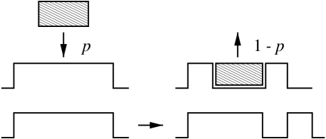
FIG. 1.: The upper panels show the deposition and evaporation of a dimer. The lower panels show diffusion of a monomer.

FIG. 2.: Monte Carlo results for the dimer model. (a) Time dependence of the surface width for $L=32,\ldots,1024$ from bottom to top. The straight line has slope $2\beta_{EW}=1/2$. (b) Saturated surface width. The straight line has slope $2\alpha_{EW}=1$. (c) and (d) Effective values for $\beta$ and $\alpha$.

FIG. 3.: (a) Time dependence of the surface width of the dimer model with diffusion, for $L=32,\ldots,512$ from bottom to top. The straight line has slope $2\beta_{EW}=1/2$. (b) Effective values of $\alpha$ for with ($\Box$) and without ($\circ$) diffusion.

FIG. 4.: EVRW (solid line) and corresponding surface (dotted line) configurations.

FIG. 5.: Exact enumeration of the total number of EVRW’s. (a) $\ln Z^{0}$ vs. $t$, (b) $\mu(t)$ vs. $1/t$, and (c) log-log plot of $-\ln[2^{-t}Z^{0}]$ vs. $t$.

FIG. 6.: Exact enumeration of the EVRW. (a) Surface width $W$. (b) Effective values of the roughness exponent $\alpha$.

FIG. 7.: Monte Carlo results for the 1D EVRW. (a) Probability distribution $P(n,t)$ at $t=32(\Box)$, $64(\circ)$, $128(\bigtriangleup)$, and $256(\bigtriangledown)$. (b) Scaling of the spreading $\Delta n$.

FIG. 8.: Scaling of $P(n,t)$ for the 1D EVRW at $t=32(\Box)$, $64(\circ)$, $128(\bigtriangleup)$, and $256(\bigtriangledown)$ according to Eq. (21). The best collapse is obtained with $1/z=0.32$. The scaling function is assumed to be of the form ${\cal F}(u)=Ae^{-B|u|^{\Delta}}$. A least square fitting yields $A=0.88$, $B=0.62$, and $\Delta=1.98$.

FIG. 9.: Crossover scaling in the EVRW. (a) and (b) Spreading of the EVRW in $d=1$ and $d=2$. (c) and (d) Scaling of the data according to Eq. (29). The broken lines have slope 1/2.

- [1] Present Address: Theoretische Physik, Universität des Saarlandes, 66041 Saarbrüken, Germany.
- [2] M. E. Fisher, J. Stat. Phys. 45, 667 (1984).
- [3] J.-P. Bouchaud and A. Georges, Phys. Rep. 195, 127 (1990).
- [4] M. den Nijs, in Phase Transitions and Critical Phenomena, vol. 12, edited by C. Domb and J. L. Lebowitz (Academic Press, 1988).
- [5] M. Kardar, G. Parisi, and Y. C. Zhang, Phys. Rev. Lett. 56, 889 (1986); T. Halpin-Healy and Y. C. Zhang, Phys. Rep. 254, 215 (1995).
- [6] H. Hinrichsen, Adv. Phys. 49, 815 (2000); W. Hwang, S. Kwon, H. Park, and H. Park, Phys. Rev. E 57, 6438 (1998).
- [7] M. Kardar and Y. C. Zhang, Phys. Rev. Lett. 58, 2087 (1987).
- [8] J. M. Kim, M. A. Moore, and A. J. Bray, Phys. Rev. A 44 2345 (1991).
- [9] G. I. Menon, M. Barma, and D. Dhar, J. Stat. Phys. 86, 1237 (1997).
- [10] J. D. Noh, H. Park, and M. den Nijs, Phys. Rev. Lett. 84, 3891 (2000).
- [11] N. Hatano and D. R. Nelson, Phys. Rev. Lett. 77, 570 (1997).
- [12] J. Feinberg and A. Zee, Phys. Rev. E 59, 6433 (1999).
- [13] R. Friedberg and J. M. Luttinger, Phys. Rev. B 12, 4460 (1975); J. M. Luttinger and R. Tao, Ann. Phys. 145, 185 (1983).
- [14] A. L. Barabási and H. E. Stanley, Fractal Concepts in Surface Growth (Cambridge University Press, Cambridge, 1995).
- [15] S. F. Edwards and D. R. Wilkinson, Proc. R. Soc. London, Ser. A 381, 17 (1982).
- [16] M. D. Grynberg, cond-mat/0004089
- [17] H. Hinrichsen and G. Ódor, Phys. Rev. Lett. 82, 1205 (1999).
- [18] P. Politi, G. Grenet, A. Marty, A. Ponchet, and J. Villain, Phys. Rep. 324, 271 (2000).
- [19] J. D. Noh, H. Park, and M. den Nijs (unpublished).
- [20] G. M. Cicuta, M. Contedini, and L. Molinari, J. Stat. Phys. 98, 685 (2000).
- [21] A. J. Guttmann, in Phase Transitions and Critical Phenomena, vol. 13, edited by C. Domb and J. L. Lebowitz (Academic Press, 1989).
- [22] M. Bauer, D. Bernard, and J.M. Luck, cond-mat/0102512.