[

Gauge Invariance and Hall Terms in the Quasiclassical Equations of Superconductivity

Takafumi Kita

Physikalisches Institute, Universität Bayreuth, 95440 Bayreuth, Germany
and
Division of Physics, Hokkaido University, Sapporo 060-0810, Japan

()

This paper presents a careful derivation of the quasiclassical equations of superconductivity so that a manifest gauge invariance is retained with respect to the space-time arguments of the quasiclassical Green’s function $\hat{g}$. The terms responsible for the Hall effect naturally appear from the derivation. The equations are applicable to clean as well as dirty superconductors for an arbitrary external frequency much smaller than the Fermi energy. Thus, they will form a basis toward a complete microscopic understanding of the Hall effect in type-II superconductors.

]

I Introduction

The Hall effect in the vortex state of type-II superconductors remains a matter of controversy after decades of intensive investigations. The early phenomenological theories of Bardeen and Stephen[1] and Nozières and Vinen[2] fail to account for the sign change of the Hall conductivity found in the vortex state of a wide variety of materials.[3, 4] Also, a debate still continues about the forces acting on a single moving vortex.[5] This state of affairs may be attributed partly to a lack of the established tractable microscopic equations with which one could test the validity of various phenomenological models numerically. Especially, the standard quasiclassical equations of superconductivity, i.e. one of the most powerful methods for nonequilibrium superfluids and superconductors,[6] have been known to be unable to describe the phenomenon.

Efforts have been made recently to include terms responsible for the Hall effect in the quasiclassical equations. Larkin and Ovchinnikov[7] incorporated higher-order effects arising from the particle-hole asymmetry near the Fermi level, but the main terms corresponding the normal-state Hall effect are still missing in their equations. Kopnin[8] obtained kinetic equations with the desired Hall terms and used them to discuss the flux-flow Hall effect.[9] However, their applicability is limited to clean superconductors with slow time variations, due to his transformation to Green’s functions [see Eq. (20) below] which may not be suitable for deriving the equations for high-frequency disturbances. More recently, Houghton and Vekhter[10] also reported an extension, but there seem to be a couple of unsatisfactory points. First, the obtained equations do not carry a manifest gauge invariance with respect to the space-time arguments of the quasiclassical Green’s function $\hat{g}$. The second point lies in their derivation process: They first define the local one-particle energy $\xi\!\equiv\!\xi({\bf p}\!-\!\frac{e}{c}{\bf A})$ which depends on the position ${\bf R}$ as well as the momentum ${\bf p}$ through the spatial dependence of the vector potential ${\bf A}\!=\!{\bf A}({\bf R})$. Whereas they expand this $\xi$ with respect to ${\bf A}$ to get the linear field dependence of the equation, the solution $\hat{g}$ to the equation is formally defined by the integral of the full Green’s function $\hat{G}$ over the unexpanded $\xi\!=\!\xi({\bf p}\!-\!\frac{e}{c}{\bf A})$. The validity of this procedure is not entirely clear.

With these observations, we here present a careful and more straightforward derivation of the quasiclassical equations which can fully describe the Hall effect of the vortex states and form a firm basis for any detailed numerical studies. A key ingredient lies in the introduction of a new transformed Green’s function [see Eq. (17) below] whose gauge change can solely be expressed with respect to the slowly varying space-time coordinate; they are different from those used by Kopnin[8] and enable us to obtain completely gauge-invariant quasiclassical equations. The idea goes back to the original work of Gor’kov[11] and was extensively used by Eilenberger[12] prior to his derivation of the quasiclassical equations.[13] On the other hand, Larkin and Ovchinnikov[14] presented a more compact derivation of the quasiclassical equations with the left-right subtraction trick without recourse to the transformed Green’s function. Those two approaches certainly provide the same equations at the lowest order of the approximation. It turns out, however, that the advantages of the two approaches have to be combined to proceed further with the gauge-invariance at every order of the approximation for a systematic derivation of the Hall terms. Indeed, the quasiclassical equations will be obtained here by applying the left-right subtraction trick to the Dyson-Gor’kov equation for the new transformed Green’s function.

This paper is organized as follows. Section II writes down the Dyson-Gor’kov equation for the conventional retarded Nambu Green’s function, followed by an introduction of a new Green’s function whose gauge change can be expressed only with respect to the center-of-mass coordinate. Section III transforms the space-time derivatives of the Dyson-Gor’kov equation into an expression of using the new Green’s function. Section IV performs a similar transformation to the self-energy part of the Dyson-Gor’kov equation. Section V collects the results of Secs. III and IV to write down the Dyson-Gor’kov equation for the transformed Green’s function, and subsequently derives the retarded quasiclassical equations by the left-right subtraction trick. Section VI presents the extension to the advanced and the Keldysh parts. Section VII concludes the paper with several remarks.

We put $\hbar\!=\!1$ throughout, and denote the light velocity, the electron charge, and the electron bare mass by $c$, $e(<0)$, and $m$, respectively.

II Green’s functions

We will consider the elements of the Nambu-Keldysh matrix[6] separately as it turns out to be more convenient than handling the matrix itself. We first focus on the retarded part to describe the derivation, and then carry out the extension to the advanced and the Keldysh parts. We hence drop the conventional superscript ^R signifying “retarded” while the distinctions are unnecessary.

Let us define a couple of retarded Green’s functions by

$$G_{\alpha\beta}(1,2)\equiv-i\theta(t_{1}\!-\!t_{2})\langle\{\psi_{\alpha}(1),\psi_{\beta}^{\dagger}(2)\}\rangle\,,\\$$ (1)

$$F_{\alpha\beta}(1,2)\equiv-i\theta(t_{1}\!-\!t_{2})\langle\{\psi_{\alpha}(1),\psi_{\beta}(2)\}\rangle\,,$$ (2)

where $1\!\equiv\!{\bf r}_{1}t_{1}$ specifies the space-time coordinate, $\alpha\beta$ are the spin indices, and $\{A,B\}\!\equiv\!AB\!+\!BA$. To suppress the spin indices we introduce $2\!\times\!2$ matrices $\underline{G}$ and $\underline{F}$ by $(\underline{G})_{\alpha\beta}\!=\!G_{\alpha\beta}$ and $(\underline{F})_{\alpha\beta}\!=\!F_{\alpha\beta}$. Using $\underline{G}$ and $\underline{F}$, we next define a $4\times 4$ Nambu matrix by[15]

$$\hat{G}(1,2)\equiv\left[\!\begin{array}[]{cc}\vspace{1mm}\underline{G}(1,2)&\underline{F}(1,2)\\ -\underline{F}^{*}(1,2)&-\underline{G}^{*}(1,2)\end{array}\!\right],$$ (5)

and the corresponding self-energy matrix by

$$\hat{\Sigma}(1,2)\equiv\left[\!\begin{array}[]{cc}\vspace{1mm}\underline{\Sigma}(1,2)&\underline{\Delta}(1,2)\\ -\underline{\Delta}^{\!*\!}(1,2)&-\underline{\Sigma}^{*\!}(1,2)\end{array}\!\right].$$ (8)

They are changed for $\psi_{\alpha}(1)\rightarrow\psi_{\alpha}(1)\exp[i\frac{e}{c}\chi(1)]$ as $\hat{G}(1,2)\rightarrow$ $\exp[i\frac{e}{c}\chi(1)\hat{\tau}_{3}]\hat{G}(1,2)\exp[-i\frac{e}{c}\chi(2)\hat{\tau}_{3}]$, where $\hat{\tau}_{3}$ is defined by

$$\hat{\tau}_{3}\equiv\left[\begin{array}[]{rr}\underline{1}&\underline{0}\\ \underline{0}&-\underline{1}\end{array}\right],$$ (11)

with $\underline{1}$ and $\underline{0}$ denoting the $2\times 2$ unit and zero matrices, respectively. They satisfy the Dyson-Gor’kov equation:

$$\left(i\frac{\partial}{\partial t_{1}}\!-\!e\Phi_{1}\hat{\tau}_{3}\right)\hat{G}(1,2)-\left[\begin{array}[]{cc}\underline{\cal H}_{1}&\underline{0}\\ \underline{0}&-\underline{\cal H}^{*}_{1}\end{array}\right]\hat{G}(1,2)$$ (14)

$$-\!\int\hat{\Sigma}(1,3)\hat{G}(3,2)d3=\delta(1-2)\hat{1}\,.$$ (15)

Here $\Phi$ is the scalar potential, $\hat{1}$ is the $4\times 4$ unit matrix, and $\underline{\cal H}_{1}$ is defined by

$$\underline{\cal H}_{1}\equiv\left[\frac{1}{2m}\left(-i\frac{\partial}{\partial{\bf r}_{1}}-\frac{e}{c}{\bf A}_{1}\right)^{\!\!2}-\mu\right]\underline{1}\,,$$ (16)

with $\mu$ the chemical potential and $\bf A$ the vector potential.

We now introduce the key quantities, i.e. a couple of new Nambu matrices, by using a nonlocal gauge transformation as

$$\hat{\bar{G}}(1,2)\equiv\exp[iI(\vec{R},\vec{r}_{1})\hat{\tau}_{3}]\hat{G}(1,2)\exp[-iI(\vec{R},\vec{r}_{2})\hat{\tau}_{3}]\,,$$ (17)

$$\hat{\bar{\Sigma}}(1,2)\equiv\exp[iI(\vec{R},\vec{r}_{1})\hat{\tau}_{3}]\hat{\Sigma}(1,2)\exp[-iI(\vec{R},\vec{r}_{2})\hat{\tau}_{3}]\,.$$ (18)

Here $\vec{r}_{1}\!\equiv\!(ct_{1},{\bf r}_{1})$ is the four vector,[16] $\vec{R}\!\equiv\!\vec{R}_{12}\!\equiv\!\frac{1}{2}(\vec{r}_{1}+\vec{r}_{2})$, and $I$ is defined by

$$I(\vec{R},\vec{r}_{1})\equiv-\frac{e}{c}\int_{\vec{r}_{1}}^{\vec{R}}\!\vec{A}(\vec{s})\cdot d\vec{s}\,,$$ (19)

where $\vec{A}\!\equiv\!(\Phi,-{\bf A})$ denotes the covariant electromagnetic potential and $d\vec{s}$ is taken along the straight line.

The quantities $\hat{\bar{G}}$ and $\hat{\bar{\Sigma}}$ defined above have a desired property that only the center-of-mass coordinate $\vec{R}$ is relevant in the gauge transformation $\psi_{\alpha}(1)\rightarrow\psi_{\alpha}(1)\exp[i\frac{e}{c}\chi(1)]$. Indeed, $\hat{\bar{G}}$ is changed as $\hat{\bar{G}}(1,2)\rightarrow\exp[i\frac{e}{c}\chi(\vec{R})\hat{\tau}_{3}]\hat{\bar{G}}(1,2)\exp[-i\frac{e}{c}\chi(\vec{R})\hat{\tau}_{3}]$. Proceeding with $\hat{\bar{G}}$ and $\hat{\bar{\Sigma}}$, we are led to the equations with a manifest gauge invariance with respect to $\vec{R}$, as seen below. Indeed, Levanda and Fleurov[17] has successfully derived normal-state kinetic equations with a manifest gauge invariance by using the component $\underline{\bar{G}}$ of Eq. (17).

It is worth pointing out the difference of the above $\hat{\bar{G}}$ from that used by Kopnin. As mentioned in Introduction, Kopnin[8] has derived kinetic equations based on a couple of transformed Green’s functions similar to Eq. (17). However, his phase factor is different from Eq. (19) as

$$I_{\rm K}(\vec{R},\vec{r}_{1})\equiv-e\int_{t_{1}}^{T}\!\Phi({\bf r}_{1}t^{\prime})\,dt^{\prime}+\frac{e}{c}\int_{{\bf r}_{1}}^{{\bf R}}\!{\bf A}({\bf r}^{\prime}t_{1})\cdot d{\bf r}^{\prime},$$ (20)

where $d{\bf r}^{\prime}$ is along the straight line; see Eq. (18) of Ref. [8]. The present $\hat{\bar{G}}$ may be more advantageous, since its gauge transformation property is expressible only with respect to $\vec{R}$. Indeed, it will enable us a more systematic and comprehensive derivation of the Hall terms.

It is convenient for later purposes to introduce the two functions:

$${\cal E}_{1}(u)\equiv\int_{0}^{1}\!d\eta\,{\rm e}^{\eta u}=\frac{{\rm e}^{u}-1}{u}\,,$$ (21)

$${\cal E}_{2}(u)\equiv\int_{0}^{1}\!d\eta\int_{0}^{\eta}\!d\zeta\,{\rm e}^{\zeta u}=\frac{{\rm e}^{u}-1-u}{u^{2}}\,.$$ (22)

Then Eq. (19) can also be written as

$$I(\vec{R},\vec{r}_{1})=\frac{e}{c}\,{\cal E}_{1}\!\!\left(\frac{\vec{r}}{2}\!\cdot\!\frac{\partial}{\partial\vec{R}}\right)\frac{\vec{r}}{2}\!\cdot\!\vec{A}(\vec{R})\,,$$ (23)

with $\vec{r}\!\equiv\!\vec{r}_{12}\!\equiv\!\vec{r}_{1}\!-\!\vec{r}_{2}$.

III Space-time derivatives

Let us rewrite the first two terms on the left-hand side of Eq. (15) with respect to $\hat{\bar{G}}$ of Eq. (17). The following identities are useful for this purpose ($j\!=\!0,1,2,3$):

$$\frac{\partial}{\partial r_{1j}}I(\vec{R},\vec{r}_{1})=\frac{e}{c}A_{j}(\vec{r}_{1})\!-\!\frac{e}{2c}A_{j}(\vec{R})$$ (24)

$$-\frac{e}{4c}\,[2{\cal E}_{1}(\hat{u})\!-\!{\cal E}_{2}(\hat{u})]\,r_{k}\!\left[\frac{\partial\vec{A}_{j}(\vec{R})}{\partial R_{k}}\!-\!\frac{\partial\vec{A}_{k}(\vec{R})}{\partial R_{j}}\right],$$ (25)

$$\frac{\partial}{\partial r_{1j}}I(\vec{R},\vec{r}_{2})=-\frac{e}{2c}A_{j}(\vec{R})$$ (26)

$$+\frac{e}{4c}{\cal E}_{2}(-\hat{u})\,r_{k}\!\left[\frac{\partial\vec{A}_{j}(\vec{R})}{\partial R_{k}}\!-\!\frac{\partial\vec{A}_{k}(\vec{R})}{\partial R_{j}}\right],$$ (27)

where $\hat{u}\equiv\frac{\vec{r}}{2}\cdot\frac{\partial}{\partial\vec{R}}$, and summations over the repeated index $k$ $(=\!0,1,2,3)$ are implied. Using the results, the gauge-invariant time and space derivatives of $\underline{G}$ are transformed as

$${\rm e}^{iI(\vec{R},\vec{r}_{1})-iI(\vec{R},\vec{r}_{2})}\left[i\frac{\partial}{\partial t_{1}}\!-\!e\Phi(\vec{r}_{1})\right]\!\underline{G}(1,2)$$ (28)

$$= \biggl{\{}i\frac{\partial}{\partial t}+\frac{i}{2}\frac{\partial}{\partial T}+\frac{e}{4}\bigl{[}\,2{\cal E}_{1}\!\left({\textstyle\frac{t}{2}\frac{\partial}{\partial T}}\right)-{\cal E}_{2}\!\left({\textstyle\frac{t}{2}\frac{\partial}{\partial T}}\right)$$ (30)

$$+{\cal E}_{2}\!\left(-{\textstyle\frac{t}{2}\frac{\partial}{\partial T}}\right)\,\bigr{]}\,{\bf E}(\vec{R})\!\cdot\!{\bf r}\biggr{\}}\underline{\bar{G}}(1,2)\,,$$

and

$${\rm e}^{iI(\vec{R},\vec{r}_{1})-iI(\vec{R},\vec{r}_{2})}\left[-i\frac{\partial}{\partial{\bf r}_{1}}\!-\!\frac{e}{c}{\bf A}(\vec{r}_{1})\right]\!\underline{G}(1,2)$$ (31)

$$= \biggl{\{}-i\frac{\partial}{\partial{\bf r}}-\frac{i}{2}\frac{\partial}{\partial{\bf R}}-\frac{e}{4}\bigl{[}\,2{\cal E}_{1}\!\left({\textstyle\frac{t}{2}\frac{\partial}{\partial T}}\right)-{\cal E}_{2}\!\left({\textstyle\frac{t}{2}\frac{\partial}{\partial T}}\right)$$ (33)

$$+{\cal E}_{2}\!\left(-{\textstyle\frac{t}{2}\frac{\partial}{\partial T}}\right)\,\bigr{]}\!\left[\,\frac{1}{c}{\bf h}(\vec{R})\!\times\!{\bf r}\!-\!{\bf E}(\vec{R})\hskip 0.85358ptt\,\right]\biggr{\}}\underline{\bar{G}}(1,2)\,,$$

where we have neglected spatial derivatives of both the electric field ${\bf E}$ and the magnetic field ${\bf h}$. Similarly, we have

$${\rm e}^{iI(\vec{R},\vec{r}_{1})+iI(\vec{R},\vec{r}_{2})}\left[i\frac{\partial}{\partial t_{1}}\!-\!e\Phi(\vec{r}_{1})\right]\!\underline{F}(1,2)$$ (34)

$$= \biggl{\{}i\frac{\partial}{\partial t}+\frac{i}{2}\frac{\partial}{\partial T}-e\Phi(\vec{R})+\frac{e}{4}\bigl{[}\,2{\cal E}_{1}\!\left({\textstyle\frac{t}{2}\frac{\partial}{\partial T}}\right)-{\cal E}_{2}\!\left({\textstyle\frac{t}{2}\frac{\partial}{\partial T}}\right)$$ (36)

$$-{\cal E}_{2}\!\left(-{\textstyle\frac{t}{2}\frac{\partial}{\partial T}}\right)\,\bigr{]}\,{\bf E}(\vec{R})\!\cdot\!{\bf r}\biggr{\}}\underline{\bar{F}}(1,2)\,,$$

and

$${\rm e}^{iI(\vec{R},\vec{r}_{1})+iI(\vec{R},\vec{r}_{2})}\left[-i\frac{\partial}{\partial{\bf r}_{1}}\!-\!\frac{e}{c}{\bf A}(\vec{r}_{1})\right]\!\underline{F}(1,2)$$ (37)

$$= \biggl{\{}-i\frac{\partial}{\partial{\bf r}}-\frac{i}{2}\frac{\partial}{\partial{\bf R}}-\frac{e}{c}{\bf A}(\vec{R})-\frac{e}{4}\bigl{[}\,2{\cal E}_{1}\!\left({\textstyle\frac{t}{2}\frac{\partial}{\partial T}}\right)-{\cal E}_{2}\!\left({\textstyle\frac{t}{2}\frac{\partial}{\partial T}}\right)$$ (39)

$$-{\cal E}_{2}\!\left(-{\textstyle\frac{t}{2}\frac{\partial}{\partial T}}\right)\,\bigr{]}\!\left[\,\frac{1}{c}{\bf h}(\vec{R})\!\times\!{\bf r}\!-\!{\bf E}(\vec{R})\hskip 0.85358ptt\,\right]\biggr{\}}\underline{\bar{F}}(1,2)\,.$$

Notice the differences of $\pm{\cal E}_{2}(-{\textstyle\frac{t}{2}\frac{\partial}{\partial T}})$ between Eqs. (30) and (36), and also between Eqs. (33) and (39).

We now introduce the Fourier transform of $\hat{\bar{G}}$ by

$$\hat{G}({\bf p}\varepsilon,{\bf R}T)\equiv\int\hat{\bar{G}}(1,2)\,{\rm e}^{-i({\bf p}\cdot{{\bf r}}-\varepsilon t)}\,d{\bf r}dt$$ (40)

$$\equiv\left[\!\begin{array}[]{cc}\vspace{1mm}\underline{G}({\bf p}\varepsilon,{\bf R}T)&\underline{F}({\bf p}\varepsilon,{\bf R}T)\\ -\underline{F}^{*\!}(-{\bf p}\!-\!\varepsilon,{\bf R}T)&-\underline{G}^{*\!}(-{\bf p}\!-\!\varepsilon,{\bf R}T)\end{array}\!\right],$$ (43)

where the arguments $\varepsilon$ and $-\varepsilon$ both have an infinitesimal positive imaginary part. We also define the gauge-invariant derivatives $\partial_{T}$ and $\mbox{\boldmath$\partial$}_{{\bf R}}$ by

$$\partial_{T}\equiv\left\{\begin{array}[]{ll}\vspace{1mm}\frac{\partial}{\partial T}&:\mbox{on $\underline{G}$, $\underline{G}^{*}$, $\underline{\Sigma}$, $\underline{\Sigma}^{*}$, ${\bf E}$, ${\bf h}$}\\ \vspace{1mm}\frac{\partial}{\partial T}\!+\!2ie\Phi(\vec{R})&:\mbox{on $\underline{F}$, $\underline{\Delta}$}\\ \frac{\partial}{\partial T}\!-\!2ie\Phi(\vec{R})&:\mbox{on $\underline{F}^{*}$, $\underline{\Delta}^{*}$}\end{array}\right.,$$ (47)

$$\mbox{\boldmath$\partial$}_{\bf R}\equiv\left\{\begin{array}[]{ll}\vspace{1mm}\frac{\partial}{\partial{\bf R}}&:\mbox{on $\underline{G}$, $\underline{G}^{*}$, $\underline{\Sigma}$, $\underline{\Sigma}^{*}$, ${\bf E}$, ${\bf h}$}\\ \vspace{1mm}\frac{\partial}{\partial{\bf R}}\!-\!i\frac{2e}{c}{\bf A}(\vec{R})&:\mbox{on $\underline{F}$, $\underline{\Delta}$}\\ \frac{\partial}{\partial{\bf R}}\!+\!i\frac{2e}{c}{\bf A}(\vec{R})&:\mbox{on $\underline{F}^{*}$, $\underline{\Delta}^{*}$}\end{array}\right..$$ (51)

Then using Eqs. (30)-(39), we can write the first two terms on the left-hand side of Eq. (15) with respect to Eqs. (43)-(51). We finally neglect terms second-order in $\mbox{\boldmath$\partial$}_{{\bf R}}$, ${\bf E}$, ${\bf h}$, and $({\bf p}-{\bf p}_{\rm F})^{2}$ with ${\bf p}_{\rm F}$ the Fermi momentum, since they are smaller than the first-order ones by an order of magnitude in “small”,[6] i.e. $(p_{\rm F}\xi_{0})^{-1}$ etc, with $\xi_{0}$ the coherence length. With these procedures, the first two terms on the left-hand side of Eq. (15) are Fourier-transformed into

$$\left(\varepsilon+\frac{i}{2}\partial_{T}\right)\hat{G}-\left[\frac{p_{\rm F}^{2}}{2m}-\mu+\frac{{\bf p}_{\rm F}}{m}\cdot({\bf p}-{\bf p}_{\rm F})\right]\hat{\tau}_{3}\hat{G}$$ (52)

$$+\frac{i}{2}\,\frac{{\bf p}_{\rm F}}{m}\cdot\mbox{\boldmath$\partial$}_{\bf R}\hat{\tau}_{3}\hat{G}$$ (53)

$$+\frac{i}{4}e\bigl{[}\,2{\cal E}_{1}\!\left({\textstyle-\frac{i}{2}\partial_{T}\partial_{{\varepsilon}}}\right)-{\cal E}_{2}\!\left(-{\textstyle\frac{i}{2}\partial_{T}\partial_{{\varepsilon}}}\right)\bigr{]}{\bf E}\cdot\mbox{\boldmath$\partial$}_{{\bf p}}\hat{\tau}_{3}\hat{G}$$ (54)

$$+\frac{i}{4}e\,{\cal E}_{2}\!\left({\textstyle\frac{i}{2}\partial_{T}\partial_{{\varepsilon}}}\right){\bf E}\cdot\mbox{\boldmath$\partial$}_{{\bf p}}\hat{G}\hat{\tau}_{3}$$ (55)

$$+\frac{i}{4}e\bigl{[}\,2{\cal E}_{1}\!\left({\textstyle-\frac{i}{2}\partial_{T}\partial_{{\varepsilon}}}\right)-{\cal E}_{2}\!\left(-{\textstyle\frac{i}{2}\partial_{T}\partial_{{\varepsilon}}}\right)\bigr{]}$$ (56)

$$\hskip 85.35826pt\times\frac{{\bf p}_{\rm F}}{m}\cdot\left(\frac{1}{c}{\bf h}\times\mbox{\boldmath$\partial$}_{{\bf p}}+{\bf E}\,\partial_{\varepsilon}\right)\hat{G}$$ (57)

$$+\frac{i}{4}e\,{\cal E}_{2}\!\left({\textstyle\frac{i}{2}\partial_{T}\partial_{{\varepsilon}}}\right)\frac{{\bf p}_{\rm F}}{m}\cdot\left(\frac{1}{c}{\bf h}\times\mbox{\boldmath$\partial$}_{{\bf p}}+{\bf E}\,\partial_{\varepsilon}\right)\hat{\tau}_{3}\hat{G}\hat{\tau}_{3}\,,$$ (58)

where $\mbox{\boldmath$\partial$}_{\bf p}\equiv\frac{\partial}{\partial{\bf p}}$, $\partial_{\varepsilon}\equiv\frac{\partial}{\partial\varepsilon}$, and ${\cal E}_{1}$ and ${\cal E}_{2}$ are defined by Eqs. (21) and (22), respectively. Here one should keep in mind that $\partial_{T}$ in ${\cal E}_{1}$ and ${\cal E}_{2}$ operates only on ${\bf E}$ and ${\bf h}$.

With no time dependence in ${\bf E}$ and ${\bf h}$, ${\cal E}_{1}\rightarrow 1$ and ${\cal E}_{2}\rightarrow\frac{1}{2}$ so that the last four terms in Eq. (58) reduce to

$$\frac{i}{8}e\,{\bf E}\cdot\mbox{\boldmath$\partial$}_{{\bf p}}(3\hat{\tau}_{3}\hat{G}+\hat{G}\hat{\tau}_{3})$$ (59)

$$+ \frac{i}{8}e\,\frac{{\bf p}_{\rm F}}{m}\cdot\left(\frac{1}{c}{\bf h}\times\mbox{\boldmath$\partial$}_{{\bf p}}+{\bf E}\,\partial_{\varepsilon}\right)(3\hat{G}+\hat{\tau}_{3}\hat{G}\hat{\tau}_{3})\,.$$ (60)

These terms are absent in the conventional derivations, which are certainly responsible for the Hall effect of both the normal and the vortex states.

Before closing the section, we compare the above result with the corresponding one derived by Kopnin.[8] Due to the difference between Eqs. (19) and (20), he obtained instead of Eq. (60) the expression:

$$\frac{i}{2}e\left[{\bf E}\cdot\mbox{\boldmath$\partial$}_{{\bf p}}+\frac{{\bf p}_{\rm F}}{m}\cdot\left(\frac{1}{c}{\bf h}\times\mbox{\boldmath$\partial$}_{{\bf p}}+{\bf E}\,\partial_{\varepsilon}\right)\right]\hat{G}\,.$$ (61)

See Eq. (23) of Ref. [8]. In addition, whereas Eq. (58) are given in terms of the gauge-invariant derivatives of Eqs. (47) and (51), terms such as $\mbox{\boldmath$\nabla$}\!{\tilde{F}}$ and ${\partial}{\tilde{F}}/{\partial t}$ appear in Kopnin’s Eq. (21). It should also be noted that Eq. (58) is free from the assumption of the slow time variations and is applicable to the cases of arbitrary external frequencies, as long as they are much smaller than the Fermi energy.

IV Self-energy terms

We next consider the following self-energy terms appearing on the left-hand side of Eq. (15):

$$\underline{\bar{J}}(1,2)\equiv\,{\rm e}^{iI(\vec{R}_{12},\vec{r}_{1})-iI(\vec{R}_{12},\vec{r}_{2})}\!\!\int\!\underline{\Sigma}(1,3)\underline{G}(3,2)\,d3\,,$$ (62)

$$\underline{\bar{K}}(1,2)\equiv{\rm e}^{iI(\vec{R}_{12},\vec{r}_{1})-iI(\vec{R}_{12},\vec{r}_{2})}\!\!\int\!\underline{\Delta}(1,3)\underline{F}^{*\!}(3,2)\,d3\,,$$ (63)

$$\underline{\bar{L}}(1,2)\equiv\,{\rm e}^{iI(\vec{R}_{12},\vec{r}_{1})+iI(\vec{R}_{12},\vec{r}_{2})}\!\!\int\!\underline{\Sigma}(1,3)\underline{F}(3,2)\,d3\,,$$ (64)

$$\underline{\bar{M}}(1,2)\equiv{\rm e}^{iI(\vec{R}_{12},\vec{r}_{1})+iI(\vec{R}_{12},\vec{r}_{2})}\!\!\int\!\underline{\Delta}(1,3)\underline{G}^{*\!}(3,2)\,d3\,.$$ (65)

Some of the main issues may be: (i) whether these terms can also be expressed with respect to the gauge-invariant derivatives of Eqs. (47) and (51); (ii) how the bare mass $m$ in Eq. (58) is changed by the interactions; (iii) whether new terms arise or not besides the last four terms in Eq. (58).

We first focus on Eq. (62). Writing it with respect to $\underline{\bar{\Sigma}}$ and $\underline{\bar{G}}$, it is transformed into an expression where $\underline{\bar{\Sigma}}\,\underline{\bar{G}}$ is multiplied by a phase factor ${\rm e}^{i\phi_{123}}$ with

$$\phi_{123}\, \equiv-\frac{e}{c}\oint_{C_{123}}\!\vec{A}(\vec{s})\cdot d\vec{s}$$ (67)

$$=-\frac{e}{2c}\int df^{jk}\left(\frac{\partial A_{k}}{\partial x^{j}}-\frac{\partial A_{j}}{\partial x^{k}}\right)\,.$$

Here the contour $C_{123}$ is given in Fig. 1(a), and we have used the Stokes theorem to obtain the second line,[16] with the infinitesimal surface element $df^{jk}$ ($j,k\!=\!0,1,2,3$) defined by

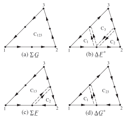
FIG. 1.: Paths of the phase integrals

$$df^{jk}\equiv (\vec{r}_{32}du)^{j}(\vec{r}_{13}dv)^{k}-(\vec{r}_{32}du)^{k}(\vec{r}_{13}dv)^{j}\,.$$ (69)

$$\hskip 22.76219pt(0\leq u\leq 1;\hskip 5.69054pt0\leq v\leq u)$$

To evaluate Eq. (67), we expand $B_{jk}\equiv\frac{\partial A_{k}}{\partial x^{j}}-\frac{\partial A_{j}}{\partial x^{k}}$ from $\vec{R}\equiv\vec{R}_{12}$ as

$$B_{jk}\bigl{(}\vec{R}+({\textstyle u-\frac{1}{2}})\vec{r}_{32}+({\textstyle v-\frac{1}{2}})\vec{r}_{13}\bigr{)}$$ (70)

$$= \sum_{n=0}^{\infty}\sum_{n^{\prime}=0}^{\infty}\frac{(u-\frac{1}{2})^{n}}{n!}\frac{(v-\frac{1}{2})^{n^{\prime}}}{n^{\prime}!}(\vec{r}_{32}\cdot\vec{\partial}_{\vec{R}})^{n}(\vec{r}_{13}\cdot\vec{\partial}_{\vec{R}})^{n^{\prime}}$$ (72)

$$\hskip 28.45274pt\times B_{jk}(\vec{R})\,.$$

We then find that, with the approximation for $\underline{\Sigma}$ adopted below in Eq. (85), the terms $(\vec{r}_{13}\cdot\vec{\partial}_{\vec{R}})^{n^{\prime}}$ with $n^{\prime}\geq 1$ can be neglected. This fact may be realized more clearly by noting that $\vec{r}_{13}\equiv(ct_{13},{\bf r}_{13})$ is transformed in Fourier space into $\varepsilon$ and ${\bf p}$ derivatives on $\underline{\Sigma}({\bf p}\varepsilon,{\bf R}T)$, and there already exists one $\vec{r}_{13}$ in the surface element as Eq. (69). Using the approximation, the integrations over $u$ and $v$ in Eq. (67) are easily performed to yield

$$\phi_{123}\, \approx-\frac{e}{4}\bigl{[}\,2{\cal E}_{1}\!\left({\textstyle\frac{t_{32}}{2}\frac{\partial}{\partial T}}\right)-{\cal E}_{2}\!\left({\textstyle\frac{t_{32}}{2}\frac{\partial}{\partial T}}\right)+{\cal E}_{2}\!\left(-{\textstyle\frac{t_{32}}{2}\frac{\partial}{\partial T}}\right)\,\bigr{]}$$ (74)

$$\times\left[\,\frac{1}{c}{\bf h}(\vec{R})\cdot({\bf r}_{13}\times{\bf r}_{32})+{\bf E}(\vec{R})\cdot({\bf r}_{13}t_{32}-t_{13}{\bf r}_{32})\,\right],$$

where ${\cal E}_{1}$ and ${\cal E}_{2}$ are defined by Eqs. (21) and (22), respectively, and we have neglected spatial derivatives of $\bf E$ and $\bf h$ once again.

We now introduce the Fourier transform of $\underline{\bar{\Sigma}}$ through

$$\underline{\bar{\Sigma}}(1,3)=\int\!\!\frac{d{\bf p}d\varepsilon}{(2\pi)^{4}}\underline{\Sigma}({\bf p}\varepsilon,{\bf R}_{13}T_{13}){\rm e}^{i({\bf p}\cdot{\bf r}_{13}-\varepsilon t_{13})}$$ (76)

$$= \exp\!\left({\textstyle\frac{{\bf r}_{32}}{2}\!\cdot\!\frac{\partial}{\partial{\bf R}}\!+\!\frac{t_{32}}{2}\frac{\partial}{\partial T}}\right)\!\!\int\!\!\frac{d{\bf p}d\varepsilon}{(2\pi)^{4}}\underline{\Sigma}({\bf p}\varepsilon,{\bf R}T){\rm e}^{i({\bf p}\cdot{\bf r}_{13}-\varepsilon t_{13})}\,.$$ (77)

Then using Eq. (LABEL:phi123-approx), we can transform Eq. (62) into

$$\underline{\bar{J}}=\int\!\!\frac{d{\bf p}d\varepsilon}{(2\pi)^{4}}\!\!\int\!\!\frac{d{\bf p}^{\prime}d\varepsilon^{\prime}}{(2\pi)^{4}}\!\!\int\!\!d{\bf r}_{3}dt_{3}\,{\rm e}^{i({\bf p}\cdot{\bf r}_{13}-\varepsilon t_{13})+i({\bf p}^{\prime}\cdot{\bf r}_{32}-\varepsilon^{\prime}t_{32})}$$ (79)

$$\times\exp\bigl{\{}\textstyle\frac{i}{4}e\bigl{[}\,2{\cal E}_{1}\!\left(-{\textstyle\frac{i}{2}\partial_{T}\partial_{\varepsilon^{\prime}}}\right)-{\cal E}_{2}\!\left(-{\textstyle\frac{i}{2}\partial_{T}\partial_{\varepsilon^{\prime}}}\right)+{\cal E}_{2}\!\left({\textstyle\frac{i}{2}\partial_{T}\partial_{\varepsilon^{\prime}}}\right)\,\bigr{]}$$ (80)

$$\hskip 34.1433pt\times\bigl{[}{\textstyle\frac{1}{c}}{\bf h}(\vec{R})\!\cdot\!(\mbox{\boldmath$\partial$}_{\bf p}\!\times\!\mbox{\boldmath$\partial$}_{{\bf p}^{\prime}})\!-\!{\bf E}(\vec{R})\!\cdot\!(\mbox{\boldmath$\partial$}_{\bf p}\partial_{\varepsilon^{\prime}}\!-\!\partial_{\varepsilon}\mbox{\boldmath$\partial$}_{{\bf p}^{\prime}})\bigr{]}\bigr{\}}$$ (81)

$$\times\exp\bigl{[}{\textstyle\frac{i}{2}(\mbox{\boldmath$\partial$}_{\bf R}\!\cdot\!\mbox{\boldmath$\partial$}_{{\bf p}^{\prime}}\!-\!\mbox{\boldmath$\partial$}_{\bf p}\!\cdot\!\mbox{\boldmath$\partial$}_{{\bf R}^{\prime}}\!-\!\partial_{T}\partial_{\varepsilon^{\prime}}\!+\!\partial_{\varepsilon}\partial_{T^{\prime}}})\bigr{]}$$ (82)

$$\times\underline{\Sigma}({\bf p}\varepsilon,{\bf R}T)\underline{G}({\bf p}^{\prime}\varepsilon^{\prime},{\bf R}^{\prime}T^{\prime})\bigl{|}_{{\bf R}^{\prime}={\bf R},T^{\prime}=T}\,,$$ (83)

where $\partial_{T}$ in ${\cal E}_{1}$ and ${\cal E}_{2}$ operates only on ${\bf E}$ and ${\bf h}$. The latter two exponentials are to be expanded to first order in $\mbox{\boldmath$\partial$}_{\bf R}$, ${\bf E}$, and ${\bf h}$, in accordance with Eq. (58). To this end, we use the following approximation for the self-energy:[18]

$$\underline{\Sigma}({\bf p}\varepsilon,{\bf R}T)\approx {\rm Re}\underline{\Sigma}({\bf p}_{\rm F}0,{\bf R}T)+\left(1\!-\!\frac{1}{a}\right)\varepsilon\,\underline{1}$$ (85)

$$+\left(\frac{{\bf v}_{\rm F}}{a}-\frac{{\bf p}_{\rm F}}{m}\right)\cdot({\bf p}\!-\!{\bf p}_{\rm F})\,\underline{1}+i{\rm Im}\underline{\Sigma}({\bf p}_{\rm F}\varepsilon,{\bf R}T)\,,$$

with $a$ the renormalization factor and ${\bf v}_{\rm F}$ the Fermi velocity.[19] We then neglect terms including ${\bf R}$ derivatives of ${\rm Re}\underline{\Sigma}({\bf p}_{\rm F}0,{\bf R}T)$ as well as $\varepsilon$ and ${\bf R}$ derivatives of ${\rm Im}\underline{\Sigma}({\bf p}_{\rm F}\varepsilon,{\bf R}T)$, since they are smaller at least by an order of magnitude in $(p_{\rm F}\xi_{0})^{-1}$. We thereby obtain the Fourier transform of Eq. (83) as

$$\underline{J}({\bf p}\varepsilon,{\bf R}T)\equiv\int\underline{\bar{J}}(1,2)\,{\rm e}^{-i({\bf p}\cdot{\bf r}-\varepsilon t)}d{\bf r}dt$$ (86)

$$= \underline{\Sigma}({\bf p}\varepsilon,{\bf R}T)\circ\underline{G}({\bf p}\varepsilon,{\bf R}T)-\frac{i}{2}\left(\frac{{\bf v}_{\rm F}}{a}-\frac{{\bf p}_{\rm F}}{m}\right)\cdot\mbox{\boldmath$\partial$}_{{\bf R}}\underline{G}$$ (91)

$$+\frac{i}{4}e\left(1\!-\!\frac{1}{a}\right)\bigl{[}\,2{\cal E}_{1}\!\left(-{\textstyle\frac{i}{2}\partial_{T}\partial_{\varepsilon}}\right)-{\cal E}_{2}\!\left(-{\textstyle\frac{i}{2}\partial_{T}\partial_{\varepsilon}}\right)$$

$$\hskip 62.59605pt+{\cal E}_{2}\!\left({\textstyle\frac{i}{2}\partial_{T}\partial_{\varepsilon}}\right)\,\bigr{]}{\bf E}\cdot\mbox{\boldmath$\partial$}_{\bf p}\underline{G}$$

$$-\frac{i}{4}e\bigl{[}\,2{\cal E}_{1}\!\left(-{\textstyle\frac{i}{2}\partial_{T}\partial_{\varepsilon}}\right)-{\cal E}_{2}\!\left(-{\textstyle\frac{i}{2}\partial_{T}\partial_{\varepsilon}}\right)+{\cal E}_{2}\!\left({\textstyle\frac{i}{2}\partial_{T}\partial_{\varepsilon}}\right)\,\bigr{]}$$

$$\hskip 14.22636pt\times\left(\frac{{\bf v}_{\rm F}}{a}-\frac{{\bf p}_{\rm F}}{m}\right)\cdot\left(\frac{1}{c}{\bf h}\!\times\!\mbox{\boldmath$\partial$}_{\bf p}\!+\!{\bf E}\,\partial_{\varepsilon}\right)\underline{G}\,,$$

where $A\circ B$ is defined by

$$A\circ B\equiv \exp\bigl{[}{\textstyle\frac{i}{2}(\partial_{\varepsilon}\partial_{T^{\prime}}}\!-\!\partial_{T}\partial_{\varepsilon^{\prime}})\bigr{]}A(\varepsilon T)B(\varepsilon^{\prime}T^{\prime})\bigl{|}_{\varepsilon^{\prime}=\varepsilon,T^{\prime}=T}\,.$$ (92)

We next consider Eq. (63). Writing it with respect to $\underline{\bar{\Delta}}$ and $\underline{\bar{F}}^{*\!}$, it is expressed as $\underline{\bar{\Delta}}\,\underline{\bar{F}}^{*\!}$ multiplied by the phase factor:

$${\rm e}^{i[I(\vec{R}_{12},\vec{r}_{1})-I(\vec{R}_{12},\vec{r}_{2})-I(\vec{R}_{13},\vec{r}_{1})-I(\vec{R}_{13},\vec{r}_{3})+I(\vec{R}_{32},\vec{r}_{3})+I(\vec{R}_{32},\vec{r}_{2})]}\,.$$

We add the four extra paths as the broken lines in Fig. 1(b) and then subtract them. This factor is thereby written as

$${\rm e}^{i(\phi_{1}+\phi_{2}+\phi_{3})+2i[I(\vec{R}_{23},\vec{R}_{12})-I(\vec{R}_{13},\vec{R}_{12})]}\,,$$

where $\phi_{j}$ ($j\!=\!1,2,3$) is defined as Eq. (67) with the contour $C_{j}$ given in Fig. 1(b). Those $\phi_{j}$’s may be transformed into expressions corresponding to Eq. (LABEL:phi123-approx), but their explicit forms will not be required below; we should only keep in mind that they all include $t_{13}$ or ${\bf r}_{13}$, as in the case of Eq. (LABEL:phi123-approx).

We now introduce the Fourier transform of $\underline{\bar{\Delta}}$ in the same way as Eq. (LABEL:S-Fourier). We also use the following identity:[20]

$$\exp[-2iI(\vec{R}_{13},\vec{R}_{12})]\exp\!\left({\textstyle\frac{{\bf r}_{32}}{2}\!\cdot\!\frac{\partial}{\partial{\bf R}}\!+\!\frac{t_{32}}{2}\frac{\partial}{\partial T}}\right)$$ (94)

$$= \exp\!\left[{\textstyle\frac{{\bf r}_{32}}{2}\!\cdot\!\left(\frac{\partial}{\partial{\bf R}}\!-\!i\frac{2e}{c}{\bf A}(\vec{R})\right)\!+\!\frac{t_{32}}{2}\!\left(\frac{\partial}{\partial T}\!+\!2ie\Phi(\vec{R})\right)}\right].$$ (95)

With these prescriptions, Eq. (63) is transformed into

$$\underline{\bar{K}}=\int\!\!\frac{d{\bf p}d\varepsilon}{(2\pi)^{4}}\!\!\int\!\!\frac{d{\bf p}^{\prime}d\varepsilon^{\prime}}{(2\pi)^{4}}\!\!\int\!\!d{\bf r}_{3}dt_{3}\,{\rm e}^{i({\bf p}\cdot{\bf r}_{13}-\varepsilon t_{13})+i({\bf p}^{\prime}\cdot{\bf r}_{32}-\varepsilon^{\prime}t_{32})}$$ (96)

$$\times{\rm e}^{i(\phi_{1}+\phi_{2}+\phi_{3})}\exp\bigl{[}{\textstyle\frac{i}{2}(\mbox{\boldmath$\partial$}_{\bf R}\!\cdot\!\mbox{\boldmath$\partial$}_{{\bf p}^{\prime}}\!-\!\mbox{\boldmath$\partial$}_{\bf p}\!\cdot\!\mbox{\boldmath$\partial$}_{{\bf R}^{\prime}}\!-\!\partial_{T}\partial_{\varepsilon^{\prime}}\!+\!\partial_{\varepsilon}\partial_{T^{\prime}}})\bigr{]}$$ (97)

$$\times\underline{\Delta}({\bf p}\varepsilon,{\bf R}T)\underline{F}^{*\!}(-{\bf p}^{\prime}\!-\!\varepsilon^{\prime},{\bf R}^{\prime}T^{\prime})\bigl{|}_{{\bf R}^{\prime}={\bf R},T^{\prime}=T}\,,$$ (98)

where $\partial_{T}$ and $\mbox{\boldmath$\partial$}_{\bf R}$ are defined by Eqs. (47) and (51), respectively. The latter two exponentials should be expanded to first order in $\mbox{\boldmath$\partial$}_{\bf R}$, ${\bf E}$, and ${\bf h}$. To this end, we use the approximation:[19]

$$\underline{\Delta}({\bf p}\varepsilon,{\bf R}T)\approx \underline{\Delta}({\bf p}_{\rm F}0,{\bf R}T)\,.$$ (99)

Compared with Eq. (85), the $\varepsilon$ and ${\bf p}-{\bf p}_{\rm F}$ expansions are stopped here at the lowest level; this difference originates from the smallness of $(p_{\rm F}\xi_{0})^{-1}$. With Eq. (99), all the ${\bf p}$ and $\varepsilon$ derivatives on $\underline{\Delta}$ vanish in Eq. (98), so that we may put $\phi_{1}+\phi_{2}+\phi_{3}=0$. Also, terms including ${\bf R}$ derivatives of $\underline{\Delta}({\bf p}_{\rm F}0,{\bf R}T)$ should be neglected as they are smaller by an order of magnitude in $(p_{\rm F}\xi_{0})^{-1}$. We thereby obtain:

$$\underline{K}({\bf p}\varepsilon,{\bf R}T)\equiv\int\underline{\bar{K}}(1,2)\,{\rm e}^{-i({\bf p}\cdot{\bf r}-\varepsilon t)}d{\bf r}dt$$ (100)

$$= \underline{\Delta}({\bf p}_{\rm F}0,{\bf R}T)\circ\underline{F}^{*\!}(-{\bf p}\!-\!\varepsilon,{\bf R}T)\,.$$ (101)

Equations (64) and (65) are transformed similarly by using the contours of the phase integrals given in Figs. 1(c) and 1(d), respectively. Especially for Eq. (64), we use the approximation:

$$\phi_{13}+\phi_{2}\equiv-\frac{e}{c}\oint_{C_{13}}\!\vec{A}(\vec{s})\cdot d\vec{s}-\frac{e}{c}\oint_{C_{2}}\!\vec{A}(\vec{s})\cdot d\vec{s}$$ (102)

$$\approx-\frac{e}{4}\bigl{[}\,2{\cal E}_{1}\!\left({\textstyle\frac{t_{32}}{2}\frac{\partial}{\partial T}}\right)-{\cal E}_{2}\!\left({\textstyle\frac{t_{32}}{2}\frac{\partial}{\partial T}}\right)-{\cal E}_{2}\!\left(-{\textstyle\frac{t_{32}}{2}\frac{\partial}{\partial T}}\right)\,\bigr{]}$$ (103)

$$\hskip 8.53581pt\times\left[\,\frac{1}{c}{\bf h}(\vec{R})\cdot({\bf r}_{13}\times{\bf r}_{32})+{\bf E}(\vec{R})\cdot({\bf r}_{13}t_{32}-t_{13}{\bf r}_{32})\,\right],$$ (104)

(105)

with $C_{13}$ and $C_{2}$ given in Fig. 1(c), which can be derived in the same way as Eq. (LABEL:phi123-approx). Notice the difference $\pm{\cal E}_{2}(-{\textstyle\frac{t_{32}}{2}\frac{\partial}{\partial T}})$ between Eqs. (LABEL:phi123-approx) and (105). Finally, the Fourier transforms of Eqs. (64) and (65) can be written in terms of the gauge-invariant derivatives of Eqs. (47) and (51) as

$$\underline{L}({\bf p}\varepsilon,{\bf R}T)\equiv\int\underline{\bar{L}}(1,2)\,{\rm e}^{-i({\bf p}\cdot{\bf r}-\varepsilon t)}d{\bf r}dt$$ (106)

$$= \underline{\Sigma}({\bf p}\varepsilon,{\bf R}T)\circ\underline{F}({\bf p}\varepsilon,{\bf R}T)-\frac{i}{2}\left(\frac{{\bf v}_{\rm F}}{a}-\frac{{\bf p}_{\rm F}}{m}\right)\cdot\mbox{\boldmath$\partial$}_{{\bf R}}\underline{F}$$ (111)

$$+\frac{i}{4}e\left(1\!-\!\frac{1}{a}\right)\bigl{[}\,2{\cal E}_{1}\!\left(-{\textstyle\frac{i}{2}\partial_{T}\partial_{\varepsilon}}\right)-{\cal E}_{2}\!\left(-{\textstyle\frac{i}{2}\partial_{T}\partial_{\varepsilon}}\right)$$

$$\hskip 62.59605pt-{\cal E}_{2}\!\left({\textstyle\frac{i}{2}\partial_{T}\partial_{\varepsilon}}\right)\,\bigr{]}{\bf E}\cdot\mbox{\boldmath$\partial$}_{\bf p}\underline{F}$$

$$-\frac{i}{4}e\bigl{[}\,2{\cal E}_{1}\!\left(-{\textstyle\frac{i}{2}\partial_{T}\partial_{\varepsilon}}\right)-{\cal E}_{2}\!\left(-{\textstyle\frac{i}{2}\partial_{T}\partial_{\varepsilon}}\right)-{\cal E}_{2}\!\left({\textstyle\frac{i}{2}\partial_{T}\partial_{\varepsilon}}\right)\,\bigr{]}$$

$$\hskip 14.22636pt\times\left(\frac{{\bf v}_{\rm F}}{a}-\frac{{\bf p}_{\rm F}}{m}\right)\cdot\left(\frac{1}{c}{\bf h}\!\times\!\mbox{\boldmath$\partial$}_{\bf p}\!+\!{\bf E}\,\partial_{\varepsilon}\right)\underline{F}\,,$$

and

$$\underline{M}({\bf p}\varepsilon,{\bf R}T)\equiv\int\underline{\bar{M}}(1,2)\,{\rm e}^{-i({\bf p}\cdot{\bf r}-\varepsilon t)}d{\bf r}dt$$ (112)

$$= \underline{\Delta}({\bf p}_{\rm F}0,{\bf R}T)\circ\underline{G}^{*\!}(-{\bf p}\!-\!\varepsilon,{\bf R}T)\,,$$ (113)

respectively.

We now collect Eqs. (91), (101), (111), and (113) into a Nambu-matrix form with respect to $\hat{G}({\bf p}\varepsilon,{\bf R}T)$ and

$$\hat{\Sigma}({\bf p}\varepsilon,{\bf R}T)\equiv\int\hat{\bar{\Sigma}}(1,2)\,{\rm e}^{-i({\bf p}\cdot{{\bf r}}-\varepsilon t)}\,d{\bf r}dt$$ (114)

$$=\left[\!\begin{array}[]{cc}\vspace{1mm}\underline{\Sigma}({\bf p}\varepsilon,{\bf R}T)&\underline{\Delta}({\bf p}\varepsilon,{\bf R}T)\\ -\underline{\Delta}^{\!\!*\!}(-{\bf p}\!-\!\varepsilon,{\bf R}T)&-\underline{\Sigma}^{*\!}(-{\bf p}\!-\!\varepsilon,{\bf R}T)\end{array}\!\right].$$ (117)

With the abbreviations $\underline{J}\equiv\underline{J}({\bf p}\varepsilon,{\bf R}T)$ and $\underline{J}^{*}\equiv\underline{J}^{*}(-{\bf p}\!-\!\varepsilon,{\bf R}T)$, etc, the third term on the left-hand side of Eq. (15) can now be written as

$$\left[\begin{array}[]{ll}-\underline{J}+\underline{K}&-\underline{L}+\underline{M}\\ -\underline{L}^{*}+\underline{M}^{*}&-\underline{J}^{*}+\underline{K}^{*}\end{array}\right]$$ (120)

$$= -\hat{\Sigma}({\bf p}\varepsilon,{\bf R}T)\circ\hat{G}({\bf p}\varepsilon,{\bf R}T)+\frac{i}{2}\left(\frac{{\bf v}_{\rm F}}{a}-\frac{{\bf p}_{\rm F}}{m}\right)\cdot\mbox{\boldmath$\partial$}_{{\bf R}}\hat{\tau}_{3}\hat{G}$$ (126)

$$-\frac{i}{4}e\!\left(1\!-\!\frac{1}{a}\right)\!\bigl{[}2{\cal E}_{1}\!\left({\textstyle-\frac{i}{2}\partial_{T}\partial_{{\varepsilon}}}\right)\!-\!{\cal E}_{2}\!\left(-{\textstyle\frac{i}{2}\partial_{T}\partial_{{\varepsilon}}}\right)\bigr{]}{\bf E}\cdot\mbox{\boldmath$\partial$}_{{\bf p}}\hat{\tau}_{3}\hat{G}$$

$$-\frac{i}{4}e\!\left(1\!-\!\frac{1}{a}\right)\!{\cal E}_{2}\!\left({\textstyle\frac{i}{2}\partial_{T}\partial_{{\varepsilon}}}\right){\bf E}\cdot\mbox{\boldmath$\partial$}_{{\bf p}}\hat{G}\hat{\tau}_{3}$$

$$+\frac{i}{4}e\,\bigl{[}\,2{\cal E}_{1}\!\left({\textstyle-\frac{i}{2}\partial_{T}\partial_{{\varepsilon}}}\right)-{\cal E}_{2}\!\left(-{\textstyle\frac{i}{2}\partial_{T}\partial_{{\varepsilon}}}\right)\bigr{]}$$

$$\hskip 56.9055pt\times\left(\frac{{\bf v}_{\rm F}}{a}\!-\!\frac{{\bf p}_{\rm F}}{m}\right)\!\cdot\!\left(\frac{1}{c}{\bf h}\!\times\!\mbox{\boldmath$\partial$}_{{\bf p}}+{\bf E}\,\partial_{\varepsilon}\right)\hat{G}$$

$$+\frac{i}{4}e\,{\cal E}_{2}\!\left({\textstyle\frac{i}{2}\partial_{T}\partial_{{\varepsilon}}}\right)\!\left(\frac{{\bf v}_{\rm F}}{a}\!-\!\frac{{\bf p}_{\rm F}}{m}\right)\!\cdot\!\left(\frac{1}{c}{\bf h}\!\times\!\mbox{\boldmath$\partial$}_{{\bf p}}+{\bf E}\,\partial_{\varepsilon}\right)\hat{\tau}_{3}\hat{G}\hat{\tau}_{3}\,,$$

with

$$\hat{\Sigma}({\bf p}\varepsilon,{\bf R}T)=\left(1\!-\!\frac{1}{a}\right)\varepsilon\,\hat{1}+\left(\frac{{\bf v}_{\rm F}}{a}-\frac{{\bf p}_{\rm F}}{m}\right)\cdot({\bf p}\!-\!{\bf p}_{\rm F})\,\hat{\tau}_{3}$$ (128)

$$\hskip 14.22636pt+\left[\begin{array}[]{cc}{\rm Re}\underline{\Sigma}({\bf p}_{\rm F}0,{\bf R}T)&\underline{\Delta}({\bf p}_{\rm F}0,{\bf R}T)\\ -\underline{\Delta}^{\!\!*}\!(-{\bf p}_{\rm F}0,{\bf R}T)&-{\rm Re}\underline{\Sigma}(-{\bf p}_{\rm F}0,{\bf R}T)\end{array}\right]$$ (131)

$$\hskip 14.22636pt+\,i\left[\begin{array}[]{cc}{\rm Im}\underline{\Sigma}({\bf p}_{\rm F}\varepsilon,{\bf R}T)&\underline{0}\\ \underline{0}&{\rm Im}\underline{\Sigma}(-{\bf p}_{\rm F}\!-\!\varepsilon,{\bf R}T)\end{array}\right]\,.$$ (134)

One should keep in mind that $\partial_{T}$ in ${\cal E}_{1}$ and ${\cal E}_{2}$ of Eq. (LABEL:HatSG) operates only on ${\bf E}$ and ${\bf h}$.

Several comments are in order before closing the section. First, Eq. (LABEL:HatSG) is expressed entirely in terms of the gauge-invariant derivatives of Eqs. (47) and (51). Second, it exactly contains those terms which turn the bare mass of Eq. (58) into the effective mass $m^{*}\equiv({\partial v_{\rm F}}/{\partial p_{\rm F}})^{-1}$. Finally, aside from this change of the bare mass into the effective mass, no new terms arise in Eq. (LABEL:HatSG) besides the last four terms of Eq. (58).

V Quasiclassical equations

Adding Eqs. (58) and (LABEL:HatSG) yields the Fourier transform of the left-hand side of Eq. (15). The corresponding right-hand side is just the unit matrix $\hat{1}$. Noting $(\!\varepsilon+\frac{i}{2}\partial_{T})\hat{G}=\varepsilon\circ\hat{G}$ with $\circ$ defined by Eq. (LABEL:circ), we obtain the left-hand Dyson-Gor’kov equation as

$$(\varepsilon\hat{1}-\hat{\sigma}\hat{\tau}_{3})\circ\hat{G}-\xi\hat{\tau}_{3}\hat{G}+\frac{i}{2}{\bf v}_{\rm F}\cdot\mbox{\boldmath$\partial$}_{{\bf R}}\hat{\tau}_{3}\hat{G}$$ (135)

$$+\frac{i}{4}e\bigl{[}2{\cal E}_{1}\!\left({\textstyle-\frac{i}{2}\partial_{T}\partial_{{\varepsilon}}}\right)\!-\!{\cal E}_{2}\!\left(-{\textstyle\frac{i}{2}\partial_{T}\partial_{{\varepsilon}}}\right)\bigr{]}{\bf E}\cdot\mbox{\boldmath$\partial$}_{{\bf p}}\hat{\tau}_{3}\hat{G}$$ (136)

$$+\frac{i}{4}e{\cal E}_{2}\!\left({\textstyle\frac{i}{2}\partial_{T}\partial_{{\varepsilon}}}\right){\bf E}\cdot\mbox{\boldmath$\partial$}_{{\bf p}}\hat{G}\hat{\tau}_{3}$$ (137)

$$+\frac{i}{4}e\,\bigl{[}\,2{\cal E}_{1}\!\left({\textstyle-\frac{i}{2}\partial_{T}\partial_{{\varepsilon}}}\right)-{\cal E}_{2}\!\left(-{\textstyle\frac{i}{2}\partial_{T}\partial_{{\varepsilon}}}\right)\bigr{]}$$ (138)

$$\hskip 56.9055pt\times{\bf v}_{\rm F}\!\cdot\!\left(\frac{1}{c}{\bf h}\!\times\!\mbox{\boldmath$\partial$}_{{\bf p}}+{\bf E}\,\partial_{\varepsilon}\right)\hat{G}$$ (139)

$$+\frac{i}{4}e\,{\cal E}_{2}\!\left({\textstyle\frac{i}{2}\partial_{T}\partial_{{\varepsilon}}}\right)\!{\bf v}_{\rm F}\!\cdot\!\left(\frac{1}{c}{\bf h}\!\times\!\mbox{\boldmath$\partial$}_{{\bf p}}+{\bf E}\,\partial_{\varepsilon}\right)\hat{\tau}_{3}\hat{G}\hat{\tau}_{3}$$ (140)

$$=a\hat{1}\,,$$ (141)

where $\xi\equiv{\bf v}_{\rm F}\cdot({\bf p}-{\bf p}_{\rm F})$, and $\hat{\sigma}$ is defined by

$$\hat{\sigma}(\hat{\bf p}\varepsilon,{\bf R}T)\equiv a\left(\frac{p_{\rm F}^{2}}{2m}-\mu\right)\hat{1}$$ (142)

$$+a\left[\begin{array}[]{cc}{\rm Re}\underline{\Sigma}({\bf p}_{\rm F}0,{\bf R}T)&\underline{\Delta}({\bf p}_{\rm F}0,{\bf R}T)\\ -\underline{\Delta}^{\!\!*}\!(-{\bf p}_{\rm F}0,{\bf R}T)&-{\rm Re}\underline{\Sigma}(-{\bf p}_{\rm F}0,{\bf R}T)\end{array}\right]\hat{\tau}_{3}$$ (145)

$$+ia\left[\begin{array}[]{cc}{\rm Im}\underline{\Sigma}({\bf p}_{\rm F}\varepsilon,{\bf R}T)&\underline{0}\\ \underline{0}&{\rm Im}\underline{\Sigma}(-{\bf p}_{\rm F}\!-\!\varepsilon,{\bf R}T)\end{array}\right]\hat{\tau}_{3}\,.$$ (148)

The corresponding right-hand equation may be derived similarly. It can also be obtained from Eq. (141) by: (i) taking its Hermitian conjugate with noting the relations $\hat{G}^{{\rm R}\dagger}({\bf p}\varepsilon,{\bf R}T)=\hat{G}^{{\rm A}}({\bf p}\varepsilon,{\bf R}T)$ and $\hat{\Sigma}^{{\rm R}\dagger}({\bf p}\varepsilon,{\bf R}T)=\hat{\Sigma}^{{\rm A}}({\bf p}\varepsilon,{\bf R}T)$, where ^A denotes “advanced”; (ii) formally changing ^A to ^R. The result is:

$$\hat{G}\circ(\varepsilon\hat{1}-\hat{\sigma}\hat{\tau}_{3})-\xi\hat{G}\hat{\tau}_{3}-\frac{i}{2}{\bf v}_{\rm F}\cdot\mbox{\boldmath$\partial$}_{{\bf R}}\hat{G}\hat{\tau}_{3}$$ (149)

$$-\frac{i}{4}e\bigl{[}2{\cal E}_{1}\!\left({\textstyle\frac{i}{2}\partial_{T}\partial_{{\varepsilon}}}\right)\!-\!{\cal E}_{2}\!\left({\textstyle\frac{i}{2}\partial_{T}\partial_{{\varepsilon}}}\right)\bigr{]}{\bf E}\cdot\mbox{\boldmath$\partial$}_{{\bf p}}\hat{G}\hat{\tau}_{3}$$ (150)

$$-\frac{i}{4}e{\cal E}_{2}\!\left({\textstyle-\frac{i}{2}\partial_{T}\partial_{{\varepsilon}}}\right){\bf E}\cdot\mbox{\boldmath$\partial$}_{{\bf p}}\hat{\tau}_{3}\hat{G}$$ (151)

$$-\frac{i}{4}e\,\bigl{[}\,2{\cal E}_{1}\!\left({\textstyle\frac{i}{2}\partial_{T}\partial_{{\varepsilon}}}\right)-{\cal E}_{2}\!\left({\textstyle\frac{i}{2}\partial_{T}\partial_{{\varepsilon}}}\right)\bigr{]}$$ (152)

$$\hskip 56.9055pt\times{\bf v}_{\rm F}\!\cdot\!\left(\frac{1}{c}{\bf h}\!\times\!\mbox{\boldmath$\partial$}_{{\bf p}}+{\bf E}\,\partial_{\varepsilon}\right)\hat{G}$$ (153)

$$-\frac{i}{4}e\,{\cal E}_{2}\!\left(-{\textstyle\frac{i}{2}\partial_{T}\partial_{{\varepsilon}}}\right)\!{\bf v}_{\rm F}\!\cdot\!\left(\frac{1}{c}{\bf h}\!\times\!\mbox{\boldmath$\partial$}_{{\bf p}}+{\bf E}\,\partial_{\varepsilon}\right)\hat{\tau}_{3}\hat{G}\hat{\tau}_{3}$$ (154)

$$=a\hat{1}\,.$$ (155)

Let us rewrite the above two equations with respect to $\hat{G}^{\prime}\!\equiv\!\hat{\tau}_{3}\hat{G}$. We next operate $\hat{\tau}_{3}$ from the left and the right sides of Eq. (155), and subtract the resulting equation from Eq. (141). We then perform the integration over $\xi$, neglecting all the $\xi$ dependences except that of $\hat{G}^{\prime}$. To this end, let us define the quasiclassical Green’s function by

$$\hat{g}(\hat{\bf p}\varepsilon,{\bf R}T)\equiv\frac{i}{a\pi}\!\int_{-\infty}^{\infty}\!\hat{\tau}_{3}\hat{G}({\bf p}\varepsilon,{\bf R}T)\cos(\xi 0_{+})\,d\xi$$ (156)

$$\hskip 19.91692pt=\left[\!\begin{array}[]{cc}\vspace{1mm}\underline{g}(\hat{\bf p}\varepsilon,{\bf R}T)&\underline{f}(\hat{\bf p}\varepsilon,{\bf R}T)\\ -\underline{f}^{*\!}(-\hat{\bf p}\!-\!\varepsilon,{\bf R}T)&-\underline{g}^{*\!}(-\hat{\bf p}\!-\!\varepsilon,{\bf R}T)\end{array}\!\right],$$ (159)

with $0_{+}$ an infinitesimal positive constant.[13, 21] We also take the following procedures to get the final equations: (i) Rewrite ${\mbox{\boldmath$\partial$}}_{{\bf p}}\!=\!{\mbox{\boldmath$\partial$}}_{{\bf p}_{\parallel}}\!+\!{\bf v}_{\rm F}\frac{\partial}{\partial\xi}$ with ${\bf p}_{\parallel}$ the component on the energy surface $\xi$. (ii) Notice ${\bf v}_{\rm F}\times{\mbox{\boldmath$\partial$}}_{{\bf p}_{\parallel}}={\bf v}_{\rm F}\times{\mbox{\boldmath$\partial$}}_{{\bf p}}$ and

$$\int_{-\infty}^{\infty}\!d\xi\,\frac{\partial^{n}}{\partial\xi^{n}}\hat{\tau}_{3}\hat{G}({\bf p}\varepsilon,{\bf R}T)\cos(\xi 0_{+})=0\,.$$

(iii) Neglect terms with ${\bf E}\cdot{\mbox{\boldmath$\partial$}}_{{\bf p}_{\parallel}}$, since they are smaller than those with ${\bf v}_{\rm F}\cdot{\bf E}\partial_{\varepsilon}$ by an order of magnitude in $(p_{\rm F}\xi_{0})^{-1}$. (iv) Make use of the integral expressions of Eqs. (21) and (22).

Thus, the quasiclassical equations are obtained as

$$[\varepsilon\hat{\tau}_{3}-\hat{\sigma},\hat{g}]_{\circ}\!+\!i{\bf v}_{\rm F}\cdot\mbox{\boldmath$\partial$}_{\bf R}\hat{g}$$ (160)

$$+\frac{i}{2}{\cal O}_{g}\{\hat{\tau}_{3},\hat{g}\}+\frac{i}{2}{\cal O}_{f}[\hat{\tau}_{3},\hat{g}]=\hat{0}\,,$$ (161)

where $[A,B]\equiv AB-BA$, $[A,B]_{\circ}\equiv A\circ B-B\circ A$, and ${\cal O}_{g}$ and ${\cal O}_{f}$ are defined by

$${\cal O}_{g}\equiv\frac{1}{2}\int_{-1}^{1}\!d\eta\biggl{\{} \left[\frac{e}{c}{\bf v}_{\rm F}\!\times\!{\bf h}\bigl{(}{\bf R},T\!-\!{\textstyle\frac{i}{2}}\eta\partial_{\varepsilon}\bigr{)}\right]\cdot\frac{\partial}{\partial{\bf p}}$$ (163)

$$+e{\bf v}_{\rm F}\!\cdot\!{\bf E}\bigl{(}{\bf R},T\!-\!{\textstyle\frac{i}{2}}\eta\partial_{\varepsilon}\bigr{)}\frac{\partial}{\partial\varepsilon}\biggr{\}}\,,$$

$${\cal O}_{f}\equiv\, \frac{1}{2}\left(\int_{0}^{1}\!-\!\int_{-1}^{0}\right)\!d\eta\biggl{\{}\left[\frac{e}{c}{\bf v}_{\rm F}\!\times\!{\bf h}\bigl{(}{\bf R},T\!-\!{\textstyle\frac{i}{2}}\eta\partial_{\varepsilon}\bigr{)}\right]\cdot\frac{\partial}{\partial{\bf p}}$$ (165)

$$\hskip 56.9055pt+e{\bf v}_{\rm F}\!\cdot\!{\bf E}\bigl{(}{\bf R},T\!-\!{\textstyle\frac{i}{2}}\eta\partial_{\varepsilon}\bigr{)}\frac{\partial}{\partial\varepsilon}\biggr{\}}\,,$$

which operate on $\underline{g}$ and $\underline{f}$ of Eq. (159), respectively. If $\bf E$ and $\bf h$ are time independent, these operators acquire the simple expressions:

$${\cal O}_{g}=\frac{e}{c}({\bf v}_{\rm F}\!\times\!{\bf h})\cdot\frac{\partial}{\partial{\bf p}}+e{\bf v}_{\rm F}\cdot{\bf E}\frac{\partial}{\partial\varepsilon}\,,$$ (166)

$${\cal O}_{f}=0\,.$$ (167)

Without the terms with ${\cal O}_{g}$ and ${\cal O}_{f}$, Eq. (161) reduces to the standard quasiclassical equations. By applying Eq. (161) to the normal state, one can show easily that Eq. (166) indeed describes the normal-state Hall effect. Thus, Eq. (161) is expected to bring a consistent understanding of the Hall effect through the superconducting transition. Notice that the same Fermi velocity ${\bf v}_{\rm F}$ is relevant in both the acceleration term $e{\bf v}_{\rm F}\cdot{\bf E}\frac{\partial}{\partial\varepsilon}$ and the Lorentz-force term $\frac{e}{c}({\bf v}_{\rm F}\!\times\!{\bf h})\cdot\frac{\partial}{\partial{\bf p}}$ of Eq. (166), even after the correlation effects have been incorporated.

A key point in the above derivation is that the terms with ${\bf E}\cdot{\mbox{\boldmath$\partial$}}_{{\bf p}_{\parallel}}$ turn out to be smaller than those with ${\bf v}_{\rm F}\cdot{\bf E}\partial_{\varepsilon}$ by an order of magnitude in $(p_{\rm F}\xi_{0})^{-1}$. Hence those terms in Eqs. (58), (83), and (98) could be neglected from the beginning. Tracing back the derivation, it then follows that the $\varepsilon$ expansion in Eqs. (85) and (99) are unnecessary, so that $\hat{\sigma}$ in Eq. (161) may have a more general $\varepsilon$ dependence than Eq. (148) as

$$\hat{\sigma}(\hat{\bf p}\varepsilon,{\bf R}T)\equiv a\left(\frac{p_{\rm F}^{2}}{2m}-\mu\right)\hat{1}+a\hat{\Sigma}({\bf p}_{\rm F}\varepsilon,{\bf R}T)\hat{\tau}_{3}\,.$$ (168)

Hence Eq. (161) can also be used, for example, for a system with a strong electron-phonon interaction where there may be a strong $\varepsilon$ dependence in $\hat{\Sigma}$.

Equation (161) carries manifest gauge invariance, i.e., it remains unchanged in the gauge transformation $\hat{g}\!\rightarrow\!\exp[i\frac{e}{c}\chi(\vec{R})\hat{\tau_{3}}]\hat{g}\exp[-i\frac{e}{c}\chi(\vec{R})\hat{\tau_{3}}]$, $\Phi\!\rightarrow\!\Phi\!-\!\frac{1}{c}\frac{\partial\chi}{\partial T}$, and ${\bf A}\!\rightarrow\!{\bf A}\!+\!\frac{\partial\chi}{\partial{\bf R}}$. This is certainly a desired property to provide a support for the validity of the present equations. Compared with the result of Kopnin,[8] Eq. (161) are more advantageous in its wide applicability, i.e. it can be used for clean as well as dirty superconductors in arbitrary external frequencies much smaller than the Fermi energy. In addition, the terms with ${\cal O}_{g}$ and ${\cal O}_{f}$ are also present in the retarded and the advanced parts of the equations; those terms were neglected by Kopnin who considered only the static case of $\omega=0$, but may have an important role in the vortex dynamics of finite external frequencies. One can also show that Eq. (161) agrees in the static limit to the equations obtained by Houghton and Vekhter,[10] if a due care is taken in the gauge choice and terms next order in $(p_{\rm F}\xi_{0})^{-1}$ (i.e. terms with ${\bf R}$ and ${\bf p}$ derivatives of $\hat{\sigma}$ and $\hat{\Delta}$) are neglected in their Eq. (53). Thus, Eq. (161) clarifies the applicability of their Eq. (53) that it is valid only in the static limit; for example, the first term in the square bracket of Eq. (165) is absent in their equation.

It follows from Eq. (161) that $\hat{\nu}\equiv\hat{g}\circ\hat{g}$ satisfies

$$[\varepsilon\hat{\tau}_{3}-\hat{\sigma},\hat{\nu}]_{\circ}+i{\bf v}_{\rm F}\cdot\mbox{\boldmath$\partial$}_{\bf R}\hat{\nu}$$ (169)

$$= -\frac{i}{2}\{\hat{g},\,{\cal O}_{g}\{\hat{\tau}_{3},\hat{g}\}\!+\!{\cal O}_{f}[{\tau}_{3},\hat{g}]\}_{\circ}\,,$$ (170)

with $\{A,B\}_{\circ}\equiv A\circ B+B\circ A$. In the absence of the right-hand terms, this equation tells us that if $\hat{\nu}=\hat{1}$ at some space point, as in the uniform cases, then ${\bf v}_{\rm F}\cdot\mbox{\boldmath$\partial$}_{\bf R}\hat{\nu}$ vanishes so that $\hat{\nu}$ does not change along the straight-line path parallel to ${\bf v}_{\rm F}$; we may thereby conclude $\hat{\nu}=\hat{1}$ everywhere. However, this normalization condition no longer holds generally in the presence of the right-hand terms. This does not cause any trouble, however, and we only have to solve Eq. (161) with imposing the condition that $\hat{\nu}\rightarrow\hat{1}$ as $\varepsilon\rightarrow\infty$ or ${\bf E}\rightarrow 0$.

VI Equations in Nambu-Keldysh space

The above result for the retarded Green’s function can easily be extended to the advanced and the Keldysh parts.[6]

Let us define the advanced Green’s functions by

$$G_{\alpha\beta}^{\rm A}(1,2) \,\equiv i\theta(t_{2}\!-\!t_{1})\langle\{\psi_{\alpha}(1),\psi_{\beta}^{\dagger}(2)\}\rangle$$ (172)

$$\,=G_{\beta\alpha}^{{\rm R}*}(2,1)\,,$$

$$F_{\alpha\beta}^{{\rm A}}(1,2) \,\equiv i\theta(t_{2}\!-\!t_{1})\langle\{\psi_{\alpha}(1),\psi_{\beta}(2)\}\rangle$$ (174)

$$\,=-F_{\beta\alpha}^{{\rm R}}(2,1)\,.$$

We also define the Fourier transform and the quasiclassical Green’s function as

$$\hat{G}^{\rm A}({\bf p}\varepsilon,{\bf R}T)\equiv\int\hat{\bar{G}}^{\rm A}(1,2)\,{\rm e}^{-i({\bf p}\cdot{{\bf r}}-\varepsilon t)}\,d{\bf r}dt$$ (175)

$$\equiv\left[\!\begin{array}[]{cc}\vspace{1mm}\underline{G}^{\rm A}({\bf p}\varepsilon,{\bf R}T)&\underline{F}^{\rm A}({\bf p}\varepsilon,{\bf R}T)\\ -\underline{F}^{{\rm A}*\!}(-{\bf p}\!-\!\varepsilon,{\bf R}T)&-\underline{G}^{{\rm A}*\!}(-{\bf p}\!-\!\varepsilon,{\bf R}T)\end{array}\!\right],$$ (178)

and

$$\hat{g}^{\rm A}(\hat{\bf p}\varepsilon,{\bf R}T)\equiv\frac{i}{a\pi}\!\int_{-\infty}^{\infty}\!\hat{\tau}_{3}\hat{G}^{\rm A}({\bf p}\varepsilon,{\bf R}T)\cos(\xi 0_{+})\,d\xi$$ (179)

$$\hskip 19.91692pt=\left[\!\begin{array}[]{cc}\vspace{1mm}\underline{g}^{\rm A}(\hat{\bf p}\varepsilon,{\bf R}T)&\underline{f}^{\rm A}(\hat{\bf p}\varepsilon,{\bf R}T)\\ -\underline{f}^{{\rm A}*\!}(-\hat{\bf p}\!-\!\varepsilon,{\bf R}T)&-\underline{g}^{{\rm A}*\!}(-\hat{\bf p}\!-\!\varepsilon,{\bf R}T)\end{array}\!\right],$$ (182)

respectively, where the arguments $\varepsilon$ and $-\varepsilon$ carry an infinitesimal negative imaginary part.

As for the Keldysh part, we start from the basic definitions:

$$G_{\alpha\beta}^{\rm K}(1,2)\equiv-i\langle[\psi_{\alpha}(1),\psi_{\beta}^{\dagger}(2)]\rangle=-G_{\beta\alpha}^{{\rm K}*}(2,1)\,,$$ (183)

$$F_{\alpha\beta}^{{\rm K}}(1,2)\equiv-i\langle[\psi_{\alpha}(1),\psi_{\beta}(2)]\rangle=-F_{\beta\alpha}^{{\rm K}}(2,1)\,.$$ (184)

We then introduce the Nambu matrix by

$$\hat{G}^{\rm K}(1,2)\equiv\left[\!\begin{array}[]{cc}\vspace{1mm}\underline{G}^{\rm K}(1,2)&\underline{F}^{\rm K}(1,2)\\ \underline{F}^{{\rm K}*}(1,2)&\underline{G}^{{\rm K}*}(1,2)\end{array}\!\right].$$ (187)

Its Fourier transform is defined by

$$\hat{G}^{\rm K}({\bf p}\varepsilon,{\bf R}T)\equiv\int\hat{\bar{G}}^{\rm K}(1,2)\,{\rm e}^{-i({\bf p}\cdot{{\bf r}}-\varepsilon t)}\,d{\bf r}dt$$ (188)

$$\equiv\left[\!\begin{array}[]{cc}\vspace{1mm}\underline{G}^{\rm K}({\bf p}\varepsilon,{\bf R}T)&\underline{F}^{\rm K}({\bf p}\varepsilon,{\bf R}T)\\ \underline{F}^{{\rm K}*\!}(-{\bf p}\!-\!\varepsilon,{\bf R}T)&\underline{G}^{{\rm K}*\!}(-{\bf p}\!-\!\varepsilon,{\bf R}T)\end{array}\!\right],$$ (191)

and the quasiclassical Green’s function by

$$\hat{g}^{\rm K}(\hat{\bf p}\varepsilon,{\bf R}T)\equiv\frac{i}{a\pi}\!\int_{-\infty}^{\infty}\!\hat{\tau}_{3}\hat{G}^{\rm K}({\bf p}\varepsilon,{\bf R}T)\cos(\xi 0_{+})\,d\xi$$ (192)

$$\hskip 19.91692pt=\left[\!\begin{array}[]{cc}\vspace{1mm}\underline{g}^{\rm K}(\hat{\bf p}\varepsilon,{\bf R}T)&\underline{f}^{\rm K}(\hat{\bf p}\varepsilon,{\bf R}T)\\ \underline{f}^{{\rm K}*\!}(-\hat{\bf p}\!-\!\varepsilon,{\bf R}T)&\underline{g}^{{\rm K}*\!}(-\hat{\bf p}\!-\!\varepsilon,{\bf R}T)\end{array}\!\right].$$ (195)

The Keldysh self-energy matrices $\hat{\Sigma}^{\rm K}$ and $\hat{\sigma}^{\rm K}$ are defined similarly as Eqs. (191) and (195), respectively.

We now introduce as usual three Keldysh matrices by

$$\check{g}\equiv\!\left[\!\begin{array}[]{cc}\vspace{1mm}\hat{g}^{\rm R}&\hat{g}^{\rm K}\\ \hat{0}&\hat{g}^{\rm A}\end{array}\!\right],\hskip 5.69054pt\check{\sigma}\equiv\!\left[\!\begin{array}[]{cc}\vspace{1mm}\hat{\sigma}^{\rm R}&\hat{\sigma}^{\rm K}\\ \hat{0}&\hat{\sigma}^{\rm A}\end{array}\!\right],\hskip 5.69054pt\check{\tau}_{3}\equiv\!\left[\!\begin{array}[]{cc}\vspace{1mm}\hat{\tau}_{3}&\hat{0}\\ \hat{0}&\hat{\tau}_{3}\end{array}\!\right].$$ (202)

Then the equations for $\hat{g}^{\rm R}$, $\hat{g}^{\rm K}$, and $\hat{g}^{\rm A}$ can be put into a compact form as

$$[\varepsilon\check{\tau}_{3}-\check{\sigma},\check{g}]_{\circ}\!+\!i{\bf v}_{\rm F}\cdot\mbox{\boldmath$\partial$}_{\bf R}\check{g}$$ (203)

$$+\frac{i}{2}{\cal O}_{g}\{\check{\tau}_{3},\check{g}\}+\frac{i}{2}{\cal O}_{f}[\check{\tau}_{3},\check{g}]=\check{0}\,,$$ (204)

where ${\cal O}_{g}$ and ${\cal O}_{f}$ are defined as Eqs. (163) and (165), respectively.

Those quasiclassical Green’s functions satisfy

$$[\hat{g}^{\rm R}(\hat{\bf p}\varepsilon,{\bf R}T)]^{\dagger}=-\hat{\tau}_{3}\hat{g}^{{\rm A}}(\hat{\bf p}\varepsilon,{\bf R}T)\hat{\tau}_{3}\,,$$ (205)

$$[\hat{g}^{\rm K}(\hat{\bf p}\varepsilon,{\bf R}T)]^{\dagger}=\hat{\tau}_{3}\hat{g}^{{\rm K}}(\hat{\bf p}\varepsilon,{\bf R}T)\hat{\tau}_{3}\,,$$ (206)

$$[\hat{g}^{\rm R}(\hat{\bf p}\varepsilon,{\bf R}T)]^{\rm T}=\hat{\tau}_{2}\hat{g}^{{\rm A}}(-\hat{\bf p}\!-\!\varepsilon,{\bf R}T)\hat{\tau}_{2}\,,$$ (207)

$$[\hat{g}^{\rm K}(\hat{\bf p}\varepsilon,{\bf R}T)]^{\rm T}=\hat{\tau}_{2}\hat{g}^{{\rm K}}(-\hat{\bf p}\!-\!\varepsilon,{\bf R}T)\hat{\tau}_{2}\,,$$ (208)

with ^T denoting the transpose. These relations originate from $[\hat{G}^{\rm R}({\bf p}\varepsilon,{\bf R}T)]^{\dagger}=\hat{G}^{\rm A}({\bf p}\varepsilon,{\bf R}T)$, $[\hat{G}^{\rm K}({\bf p}\varepsilon,{\bf R}T)]^{\dagger}=-\hat{G}^{\rm K}({\bf p}\varepsilon,{\bf R}T)$, $[\hat{G}^{\rm R}({\bf p}\varepsilon,{\bf R}T)]^{\rm T}=-\hat{\tau}_{1}\hat{G}^{\rm A}(-{\bf p}\!-\!\varepsilon,{\bf R}T)\hat{\tau}_{1}$, and $[\hat{G}^{\rm K}(\hat{\bf p}\varepsilon,{\bf R}T)]^{\rm T}=-\hat{\tau}_{1}\hat{G}^{\rm K}(-{\bf p}\!-\!\varepsilon,{\bf R}T)\hat{\tau}_{1}$, respectively. Similarly, the self-energy matrices are shown to have the symmetry:

$$[\hat{\sigma}^{\rm R}(\hat{\bf p}\varepsilon,{\bf R}T)]^{\dagger}=\hat{\tau}_{3}\hat{\sigma}^{{\rm A}}(\hat{\bf p}\varepsilon,{\bf R}T)\hat{\tau}_{3}\,,$$ (209)

$$[\hat{\sigma}^{\rm K}(\hat{\bf p}\varepsilon,{\bf R}T)]^{\dagger}=-\hat{\tau}_{3}\hat{\sigma}^{{\rm K}}(\hat{\bf p}\varepsilon,{\bf R}T)\hat{\tau}_{3}\,,$$ (210)

$$[\hat{\sigma}^{\rm R}(\hat{\bf p}\varepsilon,{\bf R}T)]^{\rm T}=\hat{\tau}_{2}\hat{\sigma}^{{\rm A}}(-\hat{\bf p}\!-\!\varepsilon,{\bf R}T)\hat{\tau}_{2}\,,$$ (211)

$$[\hat{\sigma}^{\rm K}(\hat{\bf p}\varepsilon,{\bf R}T)]^{\rm T}=\hat{\tau}_{2}\hat{\sigma}^{{\rm K}}(-\hat{\bf p}\!-\!\varepsilon,{\bf R}T)\hat{\tau}_{2}\,.$$ (212)

VII Concluding Remarks

We have presented a systematic derivation of the quasiclassical equations based a nonlocal-gauge-transformed Green’s function (17). This enabled us to retain the gauge invariance in terms of the center-of-mass coordinate $\vec{R}\!\equiv\!({\bf R}T)$ at every stage throughout the derivation. Equation (161) with Eqs. (47), (51), (LABEL:circ), (168), (163), and (165) is the main result of this paper. It naturally carries a manifest gauge invariance, i.e., it remains unchanged in the gauge transformation $\hat{g}\!\rightarrow\!\exp[i\frac{e}{c}\chi(\vec{R})\hat{\tau_{3}}]\hat{g}\exp[-i\frac{e}{c}\chi(\vec{R})\hat{\tau_{3}}]$, $\Phi\!\rightarrow\!\Phi\!-\!\frac{1}{c}\frac{\partial\chi}{\partial T}$, and ${\bf A}\!\rightarrow\!{\bf A}\!+\!\frac{\partial\chi}{\partial{\bf R}}$. This is certainly a desired property to provide a strong support for the validity of the present equations. Also, the terms responsible for the Hall effect are automatically present in the operators ${\cal O}_{g}$ and ${\cal O}_{f}$. Indeed, by applying Eq. (161) to the normal state, one recovers the normal-state Hall effect. It should also be noted that Eq. (161) is applicable to band electrons; this may be shown by using in the derivation the anisotropic self-energy $\hat{\Sigma}({\bf p}\varepsilon,{\bf R}T)$ where the effect of the periodic lattice potential is incorporated.

Compared with the results of Kopnin[8] and Houghton and Vekhter[10] which are valid only in the static limit, as discussed in the paragraph below Eq. (168), Eq. (161) is more advantageous in its wide applicability that it can be used for clean as well as dirty superconductors up to the external frequencies comparable with the energy gap. In addition, terms with ${\cal O}_{g}$ and ${\cal O}_{f}$ are also present in the retarded and the advanced parts of the equations; those terms were neglected by Kopnin who considered only the static limit of $\omega=0$, but may have an important role in the cases of finite external frequencies.

Thus, we have derived an equation which forms a firm basis for detailed studies of the Hall effect in the vortex states. Solving Eq. (161) is expected to bring a comprehensive understanding of the Hall effect in type-II superconductors.

REFERENCES

[1] J. Bardeen and M. J. Stephen,
Phys. Rev. 140, A1197 (1965).
[2]P. Nozières and W. F. Vinen, Philos. Mag. 14, 667 (1966).
[3]For an overview and references, see e.g.,
S. J. Hagen, A. W. Smith, M. Rajeswari,
J. L. Peng, Z. Y. Li, R. L. Greene, S. N. Mao, X. X. Xi,
S. Bhattacharya, Q. Li, and C. J. Lobb, Phys. Rev. B47, 1064 (1993).
[4]T. Nagaoka, Y. Matsuda, H. Obara, A. Sawa, T. Terashima,
I. Chong, M. Takano, and M. Suzuki, Phys. Rev. Lett. 80, 3594 (1998).
[5]For an overview and references, see e.g.,
E. B. Sonin, Phys. Rev. B55, 485 (1997);
M. Stone, cond-mat/9708017.
[6]For a review, see e.g., J. W. Serene and D. Rainer,
Phys. Rep. 101, 221 (1983); A. I. Larkin and Y. N. Ovchinnikov,
in Nonequilibrium Superconductivity Vol. 12,
ed. by D. N. Langenberg and A. I. Larkin (Elsevier, Amsterdam, 1986) p. 493.
[7]A. I. Larkin and Y. N. Ovchinnikov,
Phys. Rev. B51, 5965 (1995).
[8]N. B. Kopnin, J. Low Temp. Phys. 97, 157 (1994).
[9]N. B. Kopnin and A. V. Lopatin, Phys. Rev. B51, 15291 (1995).
[10] A. Houghton and I. Vekhter Phys. Rev. B57, 10831 (1998).
[11] L. P. Gor’kov, Zh. Eksp. Teor. Fiz. 36, 1918 (1959)
[Sov. Phys. JETP 9, 1364 (1959)].
[12] G. Eilenberger, Z. Phys. 190, 142 (1966).
[13] G. Eilenberger, Z. Phys. 214, 195 (1968).
[14]A. I. Larkin and Y. N. Ovchinnikov,
Zh. Eksp. Teor. Fiz. 55, 2262 (1968)
[Sov. Phys. JETP 28, 1200 (1969)].
[15]
The definitions of the Nambu Green’s functions , ,
and by Eqs. (5), (178), and (187), respectively,
are the same as those of the two review articles of Ref. [6].
On the other hand, the definitions of , ,
and by Eqs. (159), (182), and (195),