[

Dynamical turbulent flow on the Galton board with friction and magnetic field

Abstract

We study numerically and analytically the dynamics of charged particles on the Galton board, a regular lattice of disc scatters, in the presence of constant external force, magnetic field and friction. It is shown that under certain conditions friction leads to the appearance of a strange chaotic attractor. In this regime the average velocity and direction of particle flow can be effectively affected by electric and magnetic fields. We discuss the applications of these results to the charge transport in antidot superlattices and stream of suspended particles in a viscous flow through scatters.

]

It is well known that dissipation can lead to the appearance of strange chaotic attractors in nonlinear nonautonomous dynamical systems [1, 2]. In this case the energy dissipation is compensated by an external energy flow so that stationary chaotic oscillations set in on the attractor. Such an energy flow is absent in the Hamiltonian conservative systems and therefore the introduction of dissipation or friction is expected to drive the system to simple fixed points in the phase space. This rather general expectation is surly true if the system phase space is bounded. However a much richer situation appears in the case of unbounded space, where unexpectedly a strange attractor can be induced by dissipation in an originally conservative system. To investigate this situation we study the dynamics of particles on the Galton board in the presence of constant external fields and friction. This board, introduced by Galton in 1889 [3], represents a triangular lattice of rigid discs with which particles collide elastically. For the case of free particle motion, the collisions with discs make the dynamics completely chaotic on the energy surface as it was shown by Sinai [4]. In this paper we study how the dynamics of a charged particle in a presence of electric and magnetic fields is affected by a friction force ${\mathbf{F}_{f}}=-\gamma{\mathbf{v}}$ directed against particle velocity ${\mathbf{v}}$ (see Fig. 1). Without discs an external in-plane electric field $\mathbf{E}$ and a perpendicular magnetic field $\mathbf{B}$ create a stationary particle flow with the velocity ${\mathbf{v}_{f}}=({\mathbf{f}+F_{L}})/\gamma$. Here ${\mathbf{f}}=e{\mathbf{E}}$ is the effective force, ${\mathbf{F}_{L}}=e\mathbf{v_{f}\times}\mathbf{B}$ is the Lorentz force and $e,m$ are the particle charge and mass. All perturbations decay to this flow with a rate proportional to $\gamma$ so that this laminar flow can be considered as a simple attractor. The effects of friction inside one cell of the Galton board at ${\mathbf{B}}=0$ have been studied in [5] and it has been found that friction leads to the appearance of a nontrivial strange attractor. At present the effects of energy dissipation are actively investigated with the aim to construct equilibrium and nonequilibrium steady states in a deterministic way (see [6, 7] and Refs. therein). Here the Nosé-Hoover thermostat with a momentum-dependent friction coefficient allows to reach a number of interesting results with applications to molecular dynamics and nonequilibrium liquids [6]. In our studies, contrary to [5], we concentrate mainly on the spatial structure of the turbulent chaotic particle flow appearing in the presence of friction. We show that the flow direction can be efficiently affected by a magnetic field. The obtained results describe the electron dynamics in antidot superlattice which has been experimentally realized in semiconductor heterostructures [8]. In such structures the effects of classical chaos play an important role [9] and the effects of friction we discuss here can appear for relatively strong electric fields.

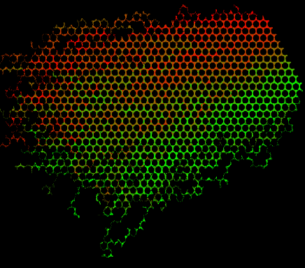
FIG. 1.: Chaotic flow on the Galton board. Here the distance between discs is $R=2.24$, ${\mathbf{f}}$ = (-0.5, -0.5), $B=2$ and $\gamma=0.1$. Initially 200 particles are distributed homogeneously along a straight line segment in the upper right corner, their color homogeneously changes from red to green along this segment.

To study numerically the dynamics of this model, we fix the disc radius $a=1$, and $e=m=1$ so that the system is characterized only by the distance $R$ between discs packed into equilateral triangles all over the $(x,y)$ plane, the friction coefficient $\gamma$, the external force of strength $f=|{\mathbf{f}}|$ and the cyclotron frequency $\omega_{c}=B$ [10]. For $R\leq R_{c}=4/\sqrt{3}$ there is no straight line, by which a particle can cross the whole plane without collisions (at $f=0,B=0,\gamma=0$), and we start the discussion from this case. The particle dynamics is simulated numerically by using the exact solution of Newton equations between collisions, and by determining the collision points with the Newton algorithm. This way the trajectories are computed with high precision, and for example for $\gamma=0$ the total energy is conserved with a relative precision of $10^{-14}$ [11]. A typical example of the chaotic flow formed by an ensemble of particle trajectories is shown in Fig. 1. To illustrate the mixing properties of the flow we attributed a color to each trajectory that allows to follow their interpenetration and spreading. This figure shows that there is a certain penetration depth of one color into another, however this depth is finite since on average the initial color repartition is still visible.

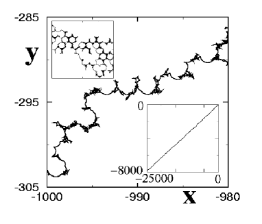
FIG. 2.: Example of a single trajectory for the case of Fig. 1 shown on small (main figure) and large (lower inset) scales. The drift velocity of the flow $v_{f}\approx 0.13$ is directed at angle $\alpha\approx 0.48$ to ${\mathbf{f}}$. Upper inset shows a single trajectory in the region $(-160\leq x\leq-140,-190\leq y\leq-170)$ for $\gamma=0.004$ with $v_{f}\approx 0.05$.

The properties of color penetration can be understood from the analysis of single trajectory dynamics. Such a typical example is presented in Fig. 2. It shows that the particle moves with an average constant velocity $v_{f}$ under some angle $\alpha$ to the external force ${\mathbf{f}}$, except for $B=0$ where $\alpha=0$. This drift velocity is constant only on average since on a smaller scale the particle moves chaotically between scatters following a strange chaotic attractor. In Fig. 2 for $\gamma=0.1$ the drift velocity is relatively large and the particle does not have enough time to move around many scatters in the direction perpendicular to the flow. As a result the penetration depth for color mixing is not very large. Surprisingly, for smaller friction, the drift velocity becomes smaller and the penetration depth increases so that the particle makes many turns around discs as it is shown in Fig. 2 for $\gamma=0.004$. This dependence is opposite to the case without scatters where $v_{f}$ drops with the $\gamma$ growth.

This result can be understood on the basis of the following physical arguments (for $B=0$ see also [5]). In the regime with weak friction the particles start to diffuse among discs in a chaotic manner with the diffusion rate $D=vl/2$ where $v$ is the particle velocity and $l$ is the mean free path [12]. For $R\sim 1$ we have $l\sim R\sim 1$ while the dependence of $l$ on $R$ will be discussed in more detail latter. During the dissipative time scale $\tau_{\gamma}=m/\gamma$ this diffusion leads to the particle displacement $\Delta r\sim\sqrt{Dm/\gamma}$ along the direction of the drift velocity ${\mathbf{v}_{f}}$. This gives the change in the potential energy $U\sim f\Delta r\cos\alpha\sim f_{ef}\sqrt{Dm/\gamma}$ where $f_{ef}=f\cos\alpha$. In the stationary regime at time $t\gg\tau_{\gamma}$, this potential energy should be comparable with the kinetic energy of the particle so that $U\sim mv^{2}$, where $v^{2}=<v^{2}_{x}+v^{2}_{y}>$ is the average velocity square. Hence

$$v^{2}\sim(f\cos\alpha)^{4/3}(l/\gamma m)^{2/3}\;\;.$$ (1)

This relation allows to determine the drift velocity of the flow ${\mathbf{v}_{f}}$. Indeed during the time $\tau_{c}$ between collisions the particle is accelerated by average forces ${\mathbf{f}}$ and ${\mathbf{F}_{L}}=e{\mathbf{v}_{f}\times B}$ that gives the average drift velocity ${\mathbf{v}_{f}}=({\mathbf{f}+F_{L}})\tau_{c}/m$. Since the dynamics is chaotic the direction of velocity is changed randomly after each collision so that ${\mathbf{v}_{f}}$ is accumulated only between collisions. The time $\tau_{c}$ is determined by the mean free path $l$ and the average velocity $v$: $\tau_{c}\;=l/v\;=2D/v^{2}$. Thus for the angle $\alpha$ between ${\mathbf{v}_{f}}$ and ${\mathbf{f}}$ we obtain the relation:

$$\tan\alpha=eB\tau_{c}/m\sim{{eB\;l^{2/3}\;\gamma^{1/3}}\over{(mf\cos\alpha)^{2/3}}}\;.$$ (2)

The amplitude of fluctuations around this direction is $\Delta r\sim\sqrt{Dm/\gamma}$ which also determines the color mixing depth (see Fig. 1).

From (1) and (2) we obtain the drift velocity amplitude

$$v_{f}=f_{ef}\tau_{c}/m\sim l^{2/3}(\gamma f_{ef}/m^{2})^{1/3}\;\;,$$ (3)

with $f_{ef}=f\cos\alpha$. For $B=0$ the particles flow in the ${\mathbf{f}}$ direction. In this case their mobility is $\mu=v_{f}/f=\tau_{c}/m=D/(mv^{2}/2)$. This is in fact the Einstein relation according to which the mobility is given by ratio of the diffusion rate to the average kinetic energy (temperature) [13]. At $B=0$ the relations (1), (2) and (3) are in the agreement with those in [5] and with the numerical data shown in Fig. 3. The values of $v_{f}$ and $v^{2}$ are obtained from one very long trajectory (with a length of $10^{3}-10^{4}\;R$ ) or 10 shorter trajectories. Within statistical fluctuations this gives the same $v_{f}$ and $v^{2}$ independent of their initial values.

The relations (1), (2), (3) allow to estimate the value of the Lyapunov exponent $\lambda$. Indeed, the particle moves with a typical velocity $v$ and as in the case of the Sinai billiard with $l\sim R\sim 1$ we have $\lambda\sim v/l$. Therefore in the regime when:

$$\gamma<\gamma_{c}\sim\sqrt{mf_{ef}/l}\;\;,$$ (4)

the value of $\lambda$ is much larger than the dissipation rate $\gamma/m$. As a result for $\gamma\ll\gamma_{c}$ the strange attractor is fat and its fractal dimension is close to the maximal dimension $4$, which is determined by the number of degrees of freedom (we remind that contrary to the nondissipative case the energy is not conserved). For $\gamma\gg\gamma_{c}$ the dissipation time $\tau_{\gamma}$ becomes much shorter than the time between collisions $\tau_{c}$. In this case the dissipation dominates chaos and the strange attractor degenerates into a simple attractor. For $\gamma<\gamma_{c}$ our numerical simulations performed with high computer accuracy show that trajectories remain chaotic for displacements from the origin being larger than $10^{5}R$. Also at $B=0$ it can be shown that $\gamma_{c}\sim mv/l\sim\sqrt{fma}/R$ for $R\gg a$ and $\gamma_{c}\sim\sqrt{mf/a^{3}}\;\Delta R$ for $\Delta R=R-2a\ll a$.

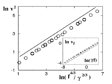
FIG. 3.: Dependences of $v^{2}$ and $v_{f}$ (inset) on $f$ and $\gamma$ for $R=2.24$, ${\mathbf{f}}/|{\mathbf{f}}|=(-1,-1)$, $B=0$ and $0.001\leq\gamma\leq 0.4$; $0.5\leq f\leq 32$: circles show numerical data and lines show the slopes from (1) (main figure) and (3) (inset).

The above changes in the mean free path $l$ at $B=0$ also affect the drift velocity of the flow through the relation (3). Indeed, for $\Delta R\ll 1$ we expect $l\sim\Delta R$ that gives $v_{f}\propto{\Delta R}^{2/3}$. This dependence is close to the numerical data shown in Fig. 4 even if the numerical value of the exponent is approximated better by $0.5$. In the other limit $R\gg 1$, we have $l\sim R^{2}/a$ that gives $v_{f}\propto R^{4/3}$. This power dependence is in a satisfactory agreement with the data in Fig. 4 although the numerical value of the exponent is closer to $1$. We attribute these small deviations in the exponent values to a restricted interval of variation in $R$. Actually we can not use very large/small values of $\Delta R$ since in these limits the value of $\gamma$ becomes comparable with $\gamma_{c}$ and chaotic attractor disappears. We note that according to our data (see Fig. 4) the strange attractor exists even in the case $R>R_{c}=4/\sqrt{3}$ when at $f=0,\gamma=0$ there are straight trajectories crossing the whole plane without collision. Apparently the contribution of these orbits is not significant if $\gamma>0$ and if $\mathbf{f}$ is not directed along these lines.

FIG. 4.: Dependence of $v_{f}$ on $\Delta R=R-2$ for $\gamma=0.1,B=0$ and ${\mathbf{f}}=(-0.5,-0.5)$: points give numerical data, lines show the slopes 0.5 and 1.

FIG. 5.: Dependence of $\tan\alpha$ on scaled magnetic field $B_{s}=B\gamma^{1/3}{f_{ef}^{-2/3}}$ from (2) with $f_{ef}=f\cos\alpha$ for $R=4$, ${\mathbf{f}}/|{\mathbf{f}}|=(-1,-1)$ and $0.125\leq B\leq 16$, $0.14\leq f\leq 5.65$, $0.002\leq\gamma\leq 0.1$. Points give numerical data, line shows the average dependence $\tan\alpha=1.6B_{s}$.

The introduction of magnetic field allows to change efficiently the direction of the flow. The numerical data for the variation of $\tan\alpha$ with the magnetic field and other system parameters are presented in Fig. 5. The average dependence is in a good agreement with the equation (2) for a large region of parameter variation where $\tan\alpha$ changes by two orders of magnitude. At the same time for moderate angles $\alpha<1$ the flow velocity $v_{f}$ is weakly affected by $B$. For example, for the case of Fig. 2, $v_{f}$ remains practically the same for $B=2$ and $B=0$ ($v_{f}\approx 0.15$). For $\alpha>1$ magnetic field starts to change significantly $v^{2}$ and $v_{f}$ in agreement with (1) and (3). While the data in Fig. 5 in average follow the dependence (2) the fluctuations around the average are rather large. Their origin becomes clear from Fig. 6 where only the magnetic field is changed. In this case, $\tan\alpha$ has a pronounced peak which is located near the value of $B$ where the cyclotron radius $r_{c}=v/B$ is equal to the disc radius. Indeed for $r_{c}>a$ a trajectory can make a full turn around a disc that allows to increase $\alpha$ and to reach a strong deviation of the global flow from the direction of the electric field. The growth of $\alpha$ leads to a drop of currant (conductivity) in the ${\mathbf{f}}$ direction and hence to the increase of resistivity. In fact, the peaks in resistivity near $r_{c}\approx a$ had been observed experimentally [8] and explained theoretically [9] in the linear response regime. Our data show that the peaks should also exist in the regime with strange chaotic attractor and relatively strong electric field where the $I-V$ characteristics become nonlinear. For a denser package of discs the above peak is still present ($R=2.24$ in Fig. 6) but it is less pronounced. It is interesting to note that in this case, $\alpha$ can even be negative so that the particles flow against the average Lorentz force. We note that the possibility of such a flow had been discussed for systems with Hamiltonian dynamical chaos in [14]. Generally for a dense disc package the contribution of resonant orbits with $r_{c}\approx a$ starts to be significant and deviations from the average dependence (2) become rather strong.

FIG. 6.: Dependence of $\tan\alpha$ on $B$ for ${\mathbf{f}}=(-0.5,-0.5)$, $\gamma=0.03$, $R=4$ (points) and $R=2.24$ (circles). Cyclotron and disc radiuses are equal at $B\approx 1.6$ where $v^{2}\approx 2.5$.

The above dynamical turbulent flow has rather interesting and unusual properties and it would be interesting to study it in experiments with antidot superlattices like in [8]. The regime we discussed should appear when the steady state velocity $v$ from (1) becomes larger than the Fermi velocity $v_{F}$ of the charge carriers. Thus, in addition to (4), the condition $v>v_{F}$ determines the threshold for appearance of a strange attractor. The experimental investigation of this phenomenon should also shade light on the role of quantum effects in such regime. We note that in the derivation of (1) - (4) we didn’t use any specific properties of the disc distribution in the plane and therefore the results remain valid for randomly distributed discs. Our study represents also certain interest for transport properties of neutral/charged particles suspended in a viscous flow streaming through a system of scatters. Indeed, a laminar stream with the velocity $v_{s}$ creates an effective force $f=v_{s}{\gamma}_{ef}$ where ${\gamma}_{ef}$ is the effective friction created by the viscosity of the liquid. Such kind of transport can be studied experimentally with viscous liquids and its investigation can contribute to a better understanding of the interplay between dissipation, turbulence and chaos.

We thank R. Klages for constructive critical remarks and for pointing to us Refs. [5, 6, 7], and W. Hoover for his stimulating interest to our work.

REFERENCES

- [1] A. Lichtenberg and M. Lieberman, Regular and chaotic dynamics, Springer, Berlin (1992).
- [2] E. Ott, Chaos in dynamical systems, Cambridge Univ. Press (1993).
- [3] F. Galton, Natural inherritance, London (1889).
- [4] I. P. Kornfeld, S. V. Fomin, and Ya. G. Sinai, Ergodic theory, Springer, Berlin (1982).
- [5] W. G. Hoover and B. Morgan, Chaos 2, 599 (1992).
- [6] W. G. Hoover, Time reversibility, computer simulation, and chaos, (World Scientific, Singapore, 1999).
- [7] R. Klages, K. Rateitschak, and G. Nicolis, Phys. Rev. Lett. 84, 4268 (2000); K. Rateitschak, R. Klages, and W. G. Hoover, J. Stat. Phys. 101, 61 (2000).
- [8] D. Weiss, M. L. Roukes, A. Menschig, P. Grambow, K. von Klitzing, and G. Weimann, Phys. Rev. Lett. 66, 2790 (1991).
- [9] R. Fleischmann, T. Geisel, and R. Ketzmerick, Phys. Rev. Lett. 68, 1367 (1992).
- [10] Dimensional analysis shows that one of these 4 parameters can be fixed but to trace their physical origin we keep all of them.
- [11] Between collisions the energy is not alternated while Newton method converges rapidly to thereof precision.
- [12] J. M. Ziman, Principles of the theory of solids, Cambridge Univ. Press (1972).
- [13] L. D. Landau and E. M. Lifshitz, Hydrodynamics, Nauka, Moscow (1986).
- [14] R. Fleischmann, T. Geisel, and R. Ketzmerick, Europhys. Lett. 25, 219 (1994).