[

Multiple-path interferometer with a single quantum obstacle

Abstract

We consider the scattering of particles by an obstacle which tunnels coherently between two positions. We show that the obstacle mimics two classical scatterers at fixed positions when the kinetic energy $\varepsilon$ of the incident particles is smaller than the tunnel splitting $\Delta$: If the obstacles are arranged in parallel, one observes an interference pattern as in the conventional double-slit experiment. If they are arranged in series, the observations conform with a Fabry-Perot interferometer. At larger $\varepsilon$ inelastic processes result in more complex interference phenomena. Interference disappears when $\varepsilon\gg\Delta$, but can be recovered if only the elastic scattering channel is detected. We discuss the realization of a quantum obstacle in mesoscopic systems.

]

In the familiar double-slit experiment a beam of particles is sent through two slits in a plate and the transmitted intensity is observed on a screen. One finds an interference pattern, thus demonstrating the coherent superposition of the two possible scattering paths. The same result is obtained for the reflection from obstacles, e. g., the bars of a reflection grating.

In these experiments the slits or bars only play a passive role. In this paper we consider scattering by a single obstacle, which, however, is by itself a quantum object with states that correspond to different locations (see Fig. 1). Allowing for superpositions of these states, we have an obstacle that is delocalized in space. Which reflection or transmission pattern is then observed on the screen? What we will demonstrate here is that the quantum obstacle may act as a collection of classical scatterers, in that one observes the corresponding interference pattern on the screen. The condition for interference is that the tunnel splitting $\Delta$ is of order or larger than the kinetic energy $\varepsilon$ of the incident particles. This suggests the interpretation that the obstacle has to tunnel quickly enough in order to give the particles a choice of the path. For $\Delta\ll\varepsilon$ the interference pattern from the obstacle disappears, but can be recovered if only the elastic scattering channel is detected. (It is also recovered by coincidence detection of the final state of the obstacle in its delocalized eigenbasis.)

The double slits or bars are two scattering elements put in parallel. We contrast this with the one-dimensional problem of two barriers arranged in series—a Fabry-Perot interferometer. The quantum analogue is an obstacle which tunnels between two locations along the propagation direction of the incident particles. We solve exactly the one-dimensional model with a repulsive contact interaction (delta-function potential $U\delta(x)$) and find transmission resonances for $\Delta\gtrsim\varepsilon$, hence again that the quantum obstacle acts as two classical obstacles if it tunnels quickly enough. In the limit of large interaction strength $U$ and sufficiently large separation between the positions of the obstacle, the transmission amplitude becomes identical to the transmission amplitude of the Fabry-Perot interferometer. In general, the transmission probability remains finite even if the barrier strength $U$ is infinite. At smaller tunnel splitting one finds a rich behavior of the transmission probability due to multiple inelastic scattering. These results are further illuminated by the delay time, a measure of the interaction time [1].

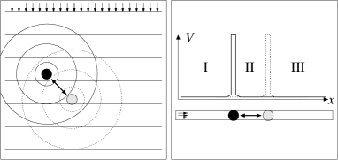
FIG. 1.: Scattering of a particle by a delocalized obstacle which tunnels between two positions (solid and shaded dot). Left panel: double slit, the obstacle provides two scattering paths in parallel. The lines indicate fronts of the wave function. Right panel: Fabry-Perot interferometer, the obstacle’s positions are arranged in series. The solid and dashed curves indicate the scattering potentials. The problem is solved by matching the waves in the regions I, II, and III.

Let us first consider the ‘parallel’ quantum scatterer in three dimensions, which hops between two positions ${\bf R}_{1}={\bf r}_{0}/2$ (internal state $|1\rangle$), ${\bf R}_{2}=-{\bf r}_{0}/2$ (internal state $|2\rangle$), with separation ${\bf r}_{0}$. The eigenstates of the scatterer are the symmetric and antisymmetric combinations $|s\rangle=2^{-1/2}(|1\rangle+|2\rangle)$ and $|a\rangle=2^{-1/2}(|1\rangle-|2\rangle)$, respectively. The corresponding eigenenergies ${\mp}\Delta/2$ differ by the tunnel splitting $\Delta>0$. (As usual we assume that the ground state is the symmetric state $|s\rangle$.) This gives rise to tunneling of the scatterer between the two positions at a frequency $\nu=\Delta/h$. The incident particle with coordinate ${\bf r}$ interacts with the scatterer at position ${\bf R}_{k}$ through a potential $V_{k}({\bf r})=V({\bf r}-{\bf R}_{k})$ which depends only on its relative position to the scatterer. The Hamiltonian describing the total system composed of the particle and the scatterer can then be written as

$$H = \frac{{\hat{\bf p}}^{2}}{2m}+\hat{W}-\frac{\Delta}{2}\left[|1\rangle\langle 2|+|2\rangle\langle 1|\right],$$ (1)

$$\hat{W} = V_{1}({\bf r})|1\rangle\langle 1|+V_{2}({\bf r})|2\rangle\langle 2|.$$ (2)

Here $\hat{\bf p}$ is the momentum operator of the particle of mass $m$. The plane-wave eigenstates $|{\bf k}\rangle$ are denoted by their wave vector ${\bf k}={\bf p}/\hbar$.

We assume that the scatterer is initially prepared in its ground state $|s\rangle$ (preparation in its excited state $|a\rangle$ is equivalent to the case $\Delta<0$; superpositions result in nonstationary behavior). In the limit of a weak interaction we can apply the Born approximation and obtain the probability of scattering from the initial state $|{\bf k}_{\rm i}\rangle$ into the final state $|{\bf k}_{\rm f}\rangle$ by summing the probabilities for each final state of the scatterer:

$$P_{{\bf k}_{\rm i}\rightarrow{\bf k}_{\rm f}} = \frac{2\pi}{\hbar}\Big{\{}\left|\langle{\bf k}_{\rm f};s|\hat{W}|s;{\bf k}_{\rm i}\rangle\right|^{2}\delta\left(\varepsilon_{\rm i}-\varepsilon_{\rm f}\right)$$ (4)

$${}+\left|\langle{\bf k}_{\rm f};a|\hat{W}|s;{\bf k}_{\rm i}\rangle\right|^{2}\delta\left(\varepsilon_{\rm i}-\varepsilon_{\rm f}-\Delta\right)\Big{\}}.$$

For of a short-ranged potential of the form $V({\bf r})=U\delta\left({\bf r}\right)$ the probability reads

$$P_{{\bf k}_{\rm i}\rightarrow{\bf k}_{\rm f}} = \frac{2\pi}{\hbar}U^{2}[\cos^{2}\left(\Delta{\bf k}\cdot{\bf r_{0}}/2\right)\delta\left(\varepsilon_{\rm i}-\varepsilon_{\rm f}\right)$$ (6)

$${}+\sin^{2}\left(\Delta{\bf k}\cdot{\bf r_{0}}/2\right)\delta\left(\varepsilon_{\rm i}-\varepsilon_{\rm f}-\Delta\right)],$$

where $\Delta{\bf k}={\bf k}_{\rm i}-{\bf k}_{\rm f}$. Interference with full contrast is observed when the energy $\varepsilon_{i}$ of the incoming particle is smaller than $\Delta$, because then the argument of the second delta function is always negative (inelastic processes are forbidden). In this situation the quantum scatterer acts as two classical scatterers of fixed positions ${\bf R}_{1}$ and ${\bf R}_{2}$, since $P_{{\bf k}_{\rm i}\rightarrow{\bf k}_{\rm f}}\sim\cos^{2}\left(\Delta{\bf k}\cdot{\bf r}_{0}\right/2)$. On the other hand, interference is lost if the kinetic energy of the incident particles $\varepsilon_{\rm i}\gg\Delta$ [2]. The interference pattern can be recovered if one only detects the elastic scattering channel (by means of energy-resolved detection at energy $\varepsilon$).

Now we turn to the ‘serial’ quantum barrier, which hops in the propagation direction of the scattered particle. In the case of one-dimensional scattering (plane-parallel barriers, or confined propagation) and for the delta-function potential $V_{1}(x)=U\delta(x-L/2)$, $V_{2}(x)=U\delta(x+L/2)$, this scattering problem can be solved exactly. [The problem is defined by the Hamiltonian given in Eq. (2) with these potentials and $\hat{\bf p}^{2}$ replaced by $\hat{p}_{x}^{2}=-\hbar^{2}\partial^{2}/\partial x^{2}$.] In order to simplify the notation we use units $\hbar^{2}/2m\equiv 1$, such that the kinetic energy $\varepsilon=k^{2}$.

Before we present the solution, let us briefly recall the results for the conventional case of immobile barriers. For a single immobile barrier of strength $U$ the transmission and reflection amplitudes at wave number $k$ are given by

$$t=\frac{1}{1+iU/2k}\quad\mbox{and}\quad r=\frac{iU/2k}{1+iU/2k},$$ (7)

respectively, such that the reflection probability approaches unity when $U\gg|k|$. When two such immobile barriers are placed in series with separation $L$ they form a Fabry-Perot interferometer, with transmission amplitude

$$t=\frac{k^{2}}{k^{2}+ikU+U^{2}[\exp(2ikL)-1]/4}.$$ (8)

For a large finesse of the interferometer ($U/k\gtrsim 1$) one finds the well-known transmission resonances close to integer values of $kL/\pi$.

The quantum scatterer is delocalized, giving rise to a number of additional resonance and interference effects. In order to explore these effects we solve the stationary scattering problem for electrons with momentum $k>0$ incident from the left, while the scatterer is prepared in the eigenstate $|s\rangle$, hence giving the total energy $E=\varepsilon-\Delta/2$. Under conservation of this energy, the electrons can be reflected or transmitted either elastically or inelastically, where in the latter case the outgoing electrons have momentum $\pm q$, with $q=\sqrt{\varepsilon-\Delta}$, and the scatterer is excited into the state $|a\rangle$.

The scattering probabilities and phase shifts can be determined via wave matching of the wavefunctions

$$\phi_{\alpha}=(a_{\alpha}e^{ikx}+b_{\alpha}e^{-ikx})|s\rangle+(c_{\alpha}e^{iqx}+d_{\alpha}e^{-iqx})|a\rangle$$ (9)

at the boundaries of the three regions $\alpha=\rm I$ for $x<-L/2$, $\alpha=\rm II$ for $-L/2<x<L/2$, and $\alpha=\rm III$ for $x>L/2$ (see Fig. 1). The resulting linear system of equations is then solved for $b_{\rm I}$, $d_{\rm I}$, $a_{\rm III}$, and $c_{\rm III}$ as a linear function of $a_{\rm I}$ (which we set to unity), under the conditions $c_{\rm I}=b_{\rm III}=d_{\rm III}=0$, because no electrons are coming in with momentum $q$, or from the right. (For the case $\varepsilon<\Delta$ we use the convention ${\rm Im}\,q>0$, so that the wavefunctions with coefficient $d_{\rm I}$ and $c_{\rm III}$ decay exponentially with the distance to the scatterer.) The coefficients (which are lengthy algebraic expressions and hence not written down here) determine the elastic and inelastic transmission and reflection probabilities by $T_{\rm el}=|a_{\rm III}|^{2}$, $T_{\rm inel}=({\rm Re}\,q/k)|c_{\rm III}|^{2}$, $R_{\rm el}=|b_{\rm I}|^{2}$, and $R_{\rm inel}=({\rm Re}\,q/k)|d_{\rm I}|^{2}$. (The inelastic scattering probability $T_{\rm inel}+R_{\rm inel}$ vanishes for $\varepsilon<\Delta$.) The coefficients also deliver the scattering phase shifts $\phi_{\rm R,T;el,inel}$, with $\phi_{\rm T;el}={\rm arg}\,a_{\rm III}$, etc, and the delay times $\tau=\hbar{\rm d}\phi/{\rm d}\varepsilon$.

Let us now discuss some special cases. In the limit $\Delta\to 0$ of slow tunneling we find

$$R=\frac{U^{2}}{4k^{2}+U^{2}},\quad R_{\rm el}=\cos^{2}(kL)R,\quad R_{\rm inel}=\sin^{2}(kL)R,$$ (10)

$$T=T_{\rm el}=\frac{4k^{2}}{4k^{2}+U^{2}},\quad T_{\rm inel}=0.$$ (11)

Qualitatively, the parameter dependence of Eq. (11) corresponds to the result in Born approximation, Eq. (6), with parallel vectors ${\bf k}_{f}\parallel{\bf k}_{i}\parallel{\bf r}_{0}$. Moreover, the total transmission and reflection probabilities are the same as for the conventional problem of a single delta function of strength $U$ [see Eq. (7)]. However, the scatterer has a finite probability $R_{\rm inel}$ to change its internal state. (This can be probed in the elastic channel if $\Delta$ is greater than the energy resolution of the detector, but still much smaller than $\varepsilon$.)

In the limit $U\gg k$ of strong scattering, according to Eq. (11) the transmittance vanishes for $\Delta=0$. In striking contrast, a finite transmission probability results for $\Delta\neq 0$ even in the limiting case $U\to\infty$, which can be interpreted as systematic avoidance of the particle and the scatterer. For $\Delta<\varepsilon$ we find in this limit the coefficients

$$a_{\rm III} = 2ik\exp(iqL)g^{-1}\,{\rm Im}\,f,$$ (12)

$$c_{\rm III} = \exp[i(k-q)L/2]a_{\rm III},$$ (13)

$$b_{\rm I} = 2qg^{-1}[i\,{\rm Im}\,f-k(\cos kL+\cos qL)],$$ (14)

$$d_{\rm I} = k\exp[-i(k+q)L/2]g^{-1}$$ (16)

$$\times[(\exp[2iqL]-1)k+(\exp[2ikL]-1)q],$$

where $f=q\exp(ikL)-k\exp(iqL)$, $g=(k+q)^{2}-f^{2}$. The proportionality between the transmission coefficients $a_{\rm III}$ and $c_{\rm III}$ in Eq. (16) entails for the elastic and inelastic transmission delay times the relation

$$\tau_{\rm T;inel}=\tau_{\rm T;el}-\frac{L}{4}\left(\frac{1}{q}-\frac{1}{k}\right)\frac{2m}{\hbar},$$ (17)

where we momentarily reintroduced the units $\hbar$, $m$.

FIG. 2.: Upper panel: Probabilities of transmission $T_{\rm el}+T_{\rm inel}$ (solid curve) and inelastic scattering $T_{\rm inel}+R_{\rm inel}$ (dashed curve) for the one-dimensional model with $U=\infty$ as a function of $kL/\pi$, for $\Delta/\varepsilon=0.4$. Lower panel: delay times $\tau_{\rm T;el}$ (solid curve), $\tau_{\rm R;el}$ (long dashes, peaks pointing upwards), and $\tau_{\rm R;inel}$ (short dashes, peaks pointing downwards), in units of $\tau_{0}=\hbar/\varepsilon$.

The corresponding probabilities of transmission and inelastic-scattering, as well as the delay times $\tau_{\rm T;el}$, $\tau_{\rm R;el}$, and $\tau_{\rm R;inel}$, are plotted in Fig. 2 as function of $kL/\pi$ for fixed $\Delta/\varepsilon=0.4$. We find a regular sequence of transmission zeros, accompanied by long delay times for the various scattering processes. The peaks of $\tau_{\rm R,el}$ point upwards, the peaks of $\tau_{\rm R,inel}$ point downwards. The transmission probability is modulated by a function $F(kL/\pi)$ [related to $f$ in Eq. (16)] with period $p=2/(1-\sqrt{1-\Delta/\varepsilon})$ and maxima at $kL/\pi=(n+1/2)p$. In the limit $\varepsilon\gg\Delta$ (where $p\simeq 4\varepsilon/\Delta$) the maxima occur when the time of flight $L/v$ of the particle between the two positions of the obstacle is an odd multiple of the tunneling time $h/2\Delta$ between these positions (the minima occur at even multiples). Close to the minima the peaks in $\tau_{\rm R,el}$ and $\tau_{\rm R,inel}$ alternate; close to the maxima they coincide.

At $\Delta=\varepsilon$ the momentum $q$ vanishes, and the inelastic scattering rate (which is proportional to ${\rm Re}\,q$) drops to zero. The transmission probability becomes

$$T=T_{\rm el}=\frac{(kL-\sin kL)^{2}}{(1+\cos kL)^{2}+(kL-\sin kL)^{2}}.$$ (18)

In the limit $kL\gg 1$ the transmission probability $T=1$. This is a remarkable observation: The scatterer becomes totally transparent although $U\to\infty$.

Another remarkable case of total transmission is found for $\Delta>\varepsilon$, where all electrons are scattered elastically. The transmission probability is now

$$T=T_{\rm el}=4k^{2}(k\sinh L|q|-|q|\sin kL)^{2}e^{-2L|q|}$$ (19)

$$\times|(k+i|q|)^{2}-e^{ikL}(ke^{-L(|q|+ik)}-i|q|)^{2}|^{-2}.$$ (20)

The delay times $\tau_{\rm T}$ and $\tau_{\rm R}$ are equal (this is a joint consequence of the unitarity of the scattering matrix and the reflection symmetry of the potential). At large length $L\gg 1/|q|$ the transmission amplitude $t$ becomes exactly identical to the transmission amplitude of the Fabry-Perot interferometer, Eq. (8), with $U$ replaced by $2|q|$. Hence, although we started out with an infinite scattering strength $U$, the finesse of the quantum version of the Fabry-Perot interferometer is finite.

FIG. 3.: Transmission probability $T$ (upper panel) and delay time $\tau$ in units of $\tau_{0}=\hbar/\varepsilon$ (lower panel), as a function of $kL/\pi$. The solid curve is the result for the quantum obstacle with scattering strength $U=\infty$ and $\Delta/\varepsilon=4$, the dashed curve (nearly indistinguishable from the solid curve) the result for the conventional Fabry-Perot interferometer (two fixed classical barriers) from Eq. (8) with $U/k=2\sqrt{3}$.

The transmission probability and the delay time is plotted for $\Delta/\varepsilon=4$ as a function of $kL/\pi$ in Fig. 3 (solid curves). The dashed curves show these quantities for two fixed classical barriers with scattering strength $U/k=2\sqrt{3}$. The comparison again demonstrates that the quantum obstacle behaves as two fixed classical scatterers when the tunnel splitting exceeds the kinetic energy.

Let us briefly discuss some implications of our results for mesoscopic systems. A possible manifestation of the delocalized scatterer is an interstitial defect, like a light atom, which hops between two energetically equivalent positions. When the thermal excitation energy is of the order of the energy barrier that the particle has to overcome, the defect jumps incoherently from one position to another. Since the potential in the system is changed after each jump, the conductance exhibits random temporal fluctuations (telegraphic noise) between two values $G_{1}$ and $G_{2}$ [3, 4, 5]. For a long measurement time one measures the time average $\langle G\rangle=(G_{1}+G_{2})/2$.

For lower temperature one enters the coherent regime in which the defect acts as a quantum obstacle. If $\Delta$ is sufficiently large the defect is in its ground state, as we have assumed in our analysis. Up to now, however, we have neglected many-body effects. The most straight-forward modification is to account for the Pauli blocking of states below the Fermi energy $E_{\rm F}$: Inelastic scattering is forbidden when the excitation energy $\varepsilon-E_{\rm F}<\Delta$. (The typical excitation energy is given by the potential drop $eV$ or by the thermal excitation energy, whatever the larger.) More intricate many-body effects arise, for example, from sequential scattering of several particles by the same quantum scatterer. If these can be neglected and inelastic processes are forbidden by Pauli blocking, we can use the Landauer formula $G=(e^{2}/h)T$ to relate the conductance to the transmission probability calculated above.

Can one also realize the serial quantum obstacle in one dimension (the Fabry-Perot interferometer)? An experimentally controllable set-up could consist of a single-channel wire placed adjacent to a double-quantum-dot device, which is tuned in resonance in the Coulomb-blockade regime. (For some experiments on double dots see Ref. [6, 7].) The quantum obstacle is the electron which occupies the two degenerate levels on the dots, and interacts with the electrons in the wire by Coulomb repulsion. However, once again for a quantitative theory one cannot neglect many-body effects. In order to circumvent these complications to some extent, one might think of injecting “hot electrons” from one end of the wire, by shooting them over an additional potential barrier. In this way the excitation energies can be restricted to a small energy interval which is well separated from the Fermi energy.

In summary, we have investigated scattering by a quantum obstacle which is delocalized in space, and found close analogies to the double slit and the Fabry-Perot interferometer. This owes to the capability of the scatterer to act as a collection of classical scatterers for fast coherent tunneling (which can be interpreted as unsuccessful resolution of the scatterer position by the particle). A striking feature of the quantum obstacle is that an infinitely high potential barrier can become transparent (which can be interpreted as successful avoidance of the particle and the scatterer). Additional regimes with a rich phenomenology have been identified, depending on the kinetic energy of the incoming particle and the tunnel frequency of the scatterer.

Recent experiments on mesoscopic structures have probed the scattering by tunable [6, 7] or spontaneously formed [8, 9] two-level systems consisting of mobile entities. These are classical obstacles at high temperatures, but could turn into quantum obstacles as the temperature is lowered. It is challenging to find signatures for having entered this new regime. We propose the appearance of interference effects like the ones discussed in this paper as such a signature. We have concentrated on a single-particle scenario which neglects many-body effects of the scattered particles, most importantly sequential scattering of several particles by the same quantum scatterer. In view of the mesoscopic applications, our results could serve as the building block for a more quantitative theory that includes these effects. This is a promising subject for further investigations.

We thank S. Bahn, H. Bouchiat, A. Georges, Y. Imry, M. Kociak, and B. Reulet for discussions. This work was supported by the Dutch Science Foundation NWO/FOM and the European Commission.

REFERENCES

- [1] E. P. Wigner, Phys. Rev. 98, 145 (1955).
- [2] C. Cohen-Tannoudji, F. Bardou, and A. Aspect, Laser spectroscopy X, eds. M. Ducloy, E. Giacobino, and G. Camy (World Scientific, Singapore, 1992).
- [3] P. Dutta and P. M. Horn, Rev. Mod. Phys. 53, 497 (1981).
- [4] M. B. Weissman, Rev. Mod. Phys. 60, 537 (1988).
- [5] Sh. Kogan, Electronic noise and fluctuations in solids (Cambridge University Press, Cambridge, 1996).
- [6] C. Livermore et al., Science 274, 1332 (1996).
- [7] T. Fujisawa et al., Science 282, 932 (1998).
- [8] H. E. van den Brom, A. I. Yanson, and J. M. van Ruitenbeek, Physica B 252, 69 (1998).
- [9] R. J. P. Keijsers, O. I. Shklyarevskii, and H. van Kempen, Physica B 253, 148 (1998).