Classical mechanism for negative magnetoresistance in two dimensions

Abstract

The classical two-dimensional problem of non-interacting electrons scattered by a static impurity potential in the presence of magnetic field is investigated both analytically and numerically. A strong negative magnetoresistance exists in such a system, due to freely circling electrons, which are not taken into account by the Boltzmann-Drude approach. A parabolic magnetoresistance is found at low fields.

PACS numbers: 05.60.+w, 73.40.-c, 73.50.Jt

——————————————————————

The negative magnetoresistance, i.e. decrease of resistance in magnetic field, frequently observed in semiconductors, as well as in metals, remained a mystery for a long time, until Altshuler et al [1] explained this phenomenon by quantum interference effects (weak localization). Extensive experimental studies of magnetoresistance, mostly in 2D semiconductor structures, have revealed that, apparently, there are two distinct types of negative magnetoresistance: (i) a small drop of resistivity observed at low fields, such that the classical parameter $\beta=\omega_{c}\tau$ is small and (ii) a relatively large (up to 50%) decrease of resistivity at $\beta\$$\buildrel>\over{\sim}$$\ 1$ or even at $\beta>>1$. Negative magnetoresistance of type (ii) is observed before the onset of Shubnikov-De Haas oscillations and may continue as a background trend after the oscillations set in (see, for example, Refs. [2-5]. In some instances, the small low-field dip of type (i) is superimposed on a smooth overall decrease of resistivity[3]. Most of the studies were devoted to the low-field magnetoresistance of type (i), which is very well explained by the weak localization correction for non-interacting electrons [1]. As to the high-field effect (ii), it is not so well understood, and is either attributed to the effect of electron-electron interaction [2], which was considered theoretically in Refs. [6], [7], or left without any explanation.

We recall that the simple Drude approach yealds zero magnetoresistance. The Drude conductivity tensor is given by:

$$\sigma_{xx}={\sigma_{0}\over\ 1+\beta^{2}},\hskip 21.68121pt\sigma_{xy}={\sigma_{0}\beta\over\ 1+\beta^{2}},$$

where $\sigma_{0}=ne^{2}\tau/m$ is the zero-field conductivity, $n$ is the electron concentration, $e$ and $m$ are the electron charge and effective mass respectively, $\tau$ is the momentum relaxation time, $\beta=\omega_{c}\tau$, and $\omega_{c}=eB/mc$ is the electron cyclotron frequency. For the resistivity tensor it follows: $\rho_{xx}=\rho_{0}=1/\sigma_{0}$, $\rho_{xy}=\beta/\sigma_{0}=B/nec$, and therefore the longitudinal resistivity is independent of the magnetic field. This result applies to degenerate electrons for which the time $\tau$, entering Eq. (1) should be taken at the Fermi energy (for nondegenerate electrons one should take into account the dependence of the scattering time $\tau$ on the electron energy, which, after averaging Eqs. (1) over the Boltzmann energy distribution, results in a positive magnetoresistance).

In this report, we draw attention to a simple classical mechanism for negative magnetoresistance. We consider non-interacting 2D electrons with a given energy (the Fermi energy) scattered by short-range impurity centers in the presence of a magnetic field perpendicular to the 2D plane, and we show that for any type of scattering a strong negative magnetoresistance should exist for $\beta>>1$. We perform computer simulations of the electron dynamics in such a system and find an excellent agreement between the numerical results and a very simple theory which is based on previously known results. Moreover we show for the first time that the magnetoresistance is parabolic at low fields.

The problem was first studied in the pioneering work of Baskin et al[8], and more recently by Bobylev et al [9], who considered specifically the 2D Lorentz model (scattering by hard disks) and derived the main results relevant for the further discussion.

The main idea put forward in Refs.[8], [9] is that, except for the case of small $\beta$, the Boltzmann-Drude approach does not work, even as a first approximation, because of the existence of ”circling” electrons, which never collide with the short-range scattering centers, the fraction of such electrons being[9]

$$P=\exp(-2\pi R/\ell)=\exp(-2\pi/\beta),$$

where $R=v/\omega_{c}$ is the cyclotron radius, $v$ is the electron (Fermi) velocity, and $\ell=v\tau$ is the electron mean free path. Contrary to the assumption intrinsic to the Boltzmann-Drude approach, an electron which happens to make one collisionless cycle will stay on its cyclotron orbit forever. The behavior of the rest of electrons (the ”wandering” electrons, in terms of Ref. [9]), whose fraction is $1-P$, is controlled by the parameter $NR^{2}$, the number of scatterers within the cyclotron orbit, $N$ being the impurity concentration. For $NR^{2}>>1$ they behave basically as predicted by the Drude theory, with an important modification: after a collision with a given scatterer there is a probability $P$ that the electron will recollide with the same scatterer without experiencing any other collisions. As a result, for $\beta>>1$ the electron will recollide with the same impurity center many times, and its trajectory will have a form of a rosette, sweeping a circular area of radius $2R$ around the impurity center [8]. Since the number of impurities inside this area, $4\pi NR^{2}$, is large, eventually the electron will collide with one of them, and thus continue its diffusion in the 2D plane. As it follows from the results of Ref. [9], frequent recollisons with the same center lead to the isotropization of scattering, so that the effective $\tau$ in Eq. (1) becomes field-dependent. This effect is absent if the scattering is isotropic.

At strong fields, when the parameter $NR^{2}$ becomes small enough, the rosettes around different scatterers do not overlap anymore, the colliding electrons become localized and give zero contribution to both $\sigma_{xx}$ and $\sigma_{xy}$. This means that a percolation transition should occur [8]. The calculated threshold is $(NR^{2})_{c}=0.36$ [9].

Thus, there are two characteristic values of the magnetic field, $B_{1}$ defined by $\omega_{c}=1/\tau$ ($\beta=1$), and $B_{2}$ defined by $\omega_{c}=v\sqrt{N}$ ($NR^{2}=1$). The ratio $B_{1}/B_{2}=(Nd^{2})^{1/2}<<1$, where $d$ is the scattering cross-section, is the small parameter of the theory.

For the simpler case of isotropic scattering and $B<<B_{2}$ ($NR^{2}>>1$), it follows from the results of Ref. [9] that the conductivity tensor for wandering electrons is given simply by the conventional Drude expressions, Eq. (1), with an additional factor $(1-P)$ in both $\sigma_{xx}$ and $\sigma_{xy}$. The circling electrons behave like free electrons with an effective concentration $nP$, giving a zero contribution to $\sigma_{xx}$, but contributing a term $P\sigma_{0}/\beta=Pnec/B$ to $\sigma_{xy}$, and this is the reason why the magnetoresistance is negative. This role of circling electrons was overlooked in Ref. [9], but was recognized later [10] (see also Refs. [11],[12]).

Thus, the conductivity tensor is given by:

$$\sigma_{xx}=\sigma_{0}{1-P\over\ 1+\beta^{2}},$$

$$\sigma_{xy}=\sigma_{0}\bigl{(}(1-P){\beta\over\ 1+\beta^{2}}+P{1\over\beta}\bigr{)},$$

As a consequence, for the resistivity tensor we obtain

$$\rho_{xx}=\rho_{0}{1-P\over 1+P^{2}/\beta^{2}},\hskip 14.45377pt\rho_{xy}=\rho_{0}\beta{1+P/\beta^{2}\over 1+P^{2}/\beta^{2}}.$$

Formulas equivalent to Eqs. (3,4) were previously obtained by Baskin and Entin [12] for scattering by randomly positioned antidots. The expression for $\rho_{xx}$ clearly exhibits negative magnetoresistance. Since the terms $P/\beta^{2}$ and $P^{2}/\beta^{2}$ are small for any $\beta$, Eqs. (4) are very similar to

$$\rho_{xx}=\rho_{0}(1-P),\hskip 14.45377pt\rho_{xy}=\rho_{0}\beta={B\over nec},$$

with an accuracy better than than 2% for $\rho_{xx}$, and better than 4% for $\rho_{xy}$. Note, that at low fields Eqs. (4,5) predict an exponentially small magnetoresistance.

Before further discussion, let us present the results of our numerical simulations. In our model a point particle (electron) with a given absolute value of its velocity, v, is scattered by disks of diameter $d$ randomly positioned on a plane inside a square box of edge length $L$ (we take $L/d=1000$ to be sure that $L$ stays more than an order of magnitude larger than the electronic mean-free path). Periodic boundary conditions are imposed at the edges of the square box. Both the hard-disk (Lorentz) model, which exhibits anisotropic scattering, and a modified model with isotropic scattering are studied. To characterize the coverage, we introduce a dimensionless concentration of scatterers $c=\pi Nd^{2}/4$, which was changed from $c=0.025$ to $c=0.2$. Studies of the percolation phenomena are beyond the scope of the present study.

FIG. 1.: Examples of simulated circling and wandering trajectories for $\beta=1$ (left) and $\beta=4$ (right) for a dimensionless impurity concentration $c=\pi Nd^{2}/4=0.1$. The actual fraction of circling electrons at $\beta=1$ is very small.

In the simulation, we first choose an initial electron position at random with an initial velocity along the $x$-direction. In a magnetic field perpendicular to the plane the electron trajectory is made of successive circular arcs of radius $R$. For each collision, we determine the intersections of the trajectory with the disk periphery (the impact point), which gives us the impact parameter, $b$, and calculate the scattering angle, $\phi$, accordingly. We follow the electron velocities $v_{x}(t)$ and $v_{y}(t)$ during a time $t=20\tau$ sufficient to get reliable results for the integral below, and calculate the components of the diffusion tensor by the standard formula:

$$D_{ij}={1\over 2}\int_{0}^{\infty}<v_{i}(0)v_{j}(t)>dt.$$

For each value of field and disk concentration we take the average over $10^{2}$ independent disk configurations, and, for each configuration, over $10^{6}$ independent trials for the initial electron position. Of course, at $B=0$, the trajectories are straight-line segments and $D_{xy}$ should vanish (this provides a nice test for the numerical precision). The conductivity tensor being proportional to the diffusion tensor, the components of the resistivity $\rho_{ij}$ are calculated as $D_{ij}/(D_{xx}^{2}+D_{xy}^{2})$, with an appropriate normalization. For the Lorentz model numerical calculations of this type were previously performed [11] with an emphasis on the percolation phenomenon.

Fig. 1 shows examples of simulated circling and wandering trajectories for two values of magnetic field. The circling electrons give undamped oscillating contributions to the velocity correlation functions in Eq. (6), accordingly, the integral in Eq. (6), strictly speaking, does not converge at $t=\infty$, but is an oscillating function of the upper limit. An average over these oscillations is performed. The same result could be obtained if a small damping of these oscillations were introduced (due, for example, to weak phonon scattering).

The numerical results for $\rho_{xx}$ as a function of $\beta$ for the model with isotropic scattering are presented in Fig. 2 (top). The resistivity is normalized to the Boltzmann-Drude zero-field value, $\rho_{0}$. The thick line is the theoretical curve predicted by Eq. (4). One can see that the theoretical and numerical curves are qualitatively similar and the quantitative agreement becomes better as $c$ decreases. In the limit $c\rightarrow 0$ the numerical results converge to the theoretical curve, as they should [13].

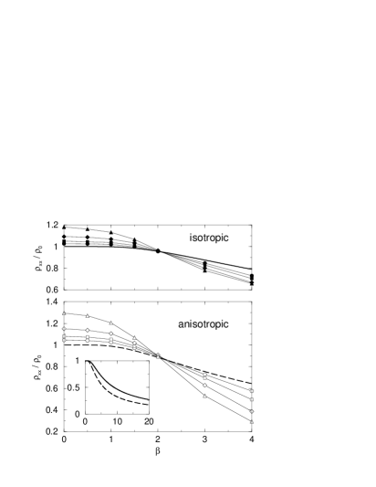
FIG. 2.: Numerical results for the resistivity as a function of $\beta=\omega_{c}\tau$ for different impurity concentrations, compared to the theoretical curve given by Eq. (4) for the isotropic scattering model (top) and for the Lorentz model with anisotropic scattering (bottom). Circles, squares, diamonds, and triangles correspond to $c=0.025,0.05,0.1,0.2$, respectively. The continuous and dashed thick lines are the theoretical curves in the isotropic and anisotropic cases, respectively, and they are depicted in the inset on a larger scale. Note the surprising crossings at $\beta=2$.

Note that for finite $c$ the value of the zero-field resistivity is higher than the Boltzmann value $\rho_{0}$. The relative correction for small $c$ is proportional to $c\ln(1/c)$ and is due to recollisions with the same impurity, which are not accounted for by the Boltzmann equation [14]. Note also, that the numerical results for finite $c$ approach the limiting theoretical curve from above for $\beta<2$, and from below for $\beta>2$. This may be qualitatively explained as follows. On the one hand, at small $\beta$ the resistivity for finite $c$ is higher than the $c\rightarrow 0$ Boltzmann value due to the $c\ln(1/c)$ correction. We have found analytically that in magnetic field this correction decreases quadratically in $\beta$, thus giving a parabolic magnetoresistance proportional to $c\beta^{2}\sim 1/NR^{2}$. On the other hand, at large $\beta$ we are on the way to the percolation threshold, where $\rho_{xx}$ (but not $\rho_{xy}$!) becomes zero. So, obviously, for large $\beta$ and finite $c$ the resistivity should be lower than the limiting value given by Eq. (4) [13].

Fig. 2 (bottom) displays quite similar results obtained for the hard disk Lorentz model (anisotropic scattering). The theoretical curve (thick dashed line) was calculated using the results of Ref. [9] for the wandering electrons and adding the contribution of circling electrons, as explained above. In both cases all the numerical curves for different $c$ cross the limiting theoretical curve at the same point $\beta=2$ (within our numerical precision). We have no explanation for this surprising finding so far.

One of the reasons, why the finite $c$ corrections are of interest, is that Eq. (4) predicts exponentially small magnetoresistance for small values of $\beta$. Corrections to this formula make the magnetic field dependence parabolic and thus define the magnetoresistance at low fields. In order to isolate the $1/NR^{2}$ terms in magnetoresistance, we look at the difference

$$\delta=\bigl{(}{\rho_{xx}(B)-\rho_{xx}(0)\over\rho_{xx}(0)}\bigr{)}_{num}-\bigl{(}{\rho_{xx}(B)-\rho_{xx}(0)\over\rho_{xx}(0)}\bigr{)}_{th}.$$

Here the second term in the right hand side is the normalized magnetoresistance, given by Eq. (4) for isotropic scattering, or by a similar formula taking care of the magnetic field dependence of $\tau$ for the anisotropic case. This term represents the limit $NR^{2}\rightarrow 0$. The first term is the normalized magnetoresistance found numerically.

This difference, as a function of $1/NR^{2}$ is presented in Fig. 3 for both the isotropic and anisotropic scattering and for different values of $c$. One can see that all the calculated points reasonably fit a universal linear dependence, which corresponds to a quadratic dependence on magnetic field. While such a dependence for small $\beta$ could be anticipated, it is surprising that it persists for quite large values of $\beta$. Thus at low magnetic field ($\beta<1$) the normalized resistivity behaves like $1-0.15/NR^{2}$, the slope being deduced from Fig. 3. For $\beta\$$\buildrel>\over{\sim}$$\ 1$ the magnetoresistance is well described by Eqs. (4,5) or, for anisotropic scattering, by similar formulas, which take care of the magnetic field dependence of $\tau$.

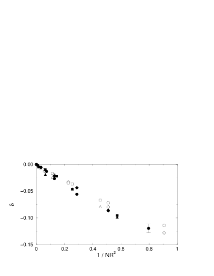
FIG. 3.: The difference, $\delta$, between normalized magnetoresistances, calculated in the limit $NR^{2}\rightarrow\infty$, and obtained numerically (see Eq. (7)) for the isotropic (empty symbols) and anisotropic (filled symbols) models, as a function of the square of the dimensionless field $(B/B_{2})^{2}=1/NR^{2}$. Circles, squares, diamonds, and triangles correspond to $c=0.025,0.05,0.1,0.2$, respectively. The data fit a linear dependence $\delta=-0.15/NR^{2}$.

The classical approach is justified if the number of Landau levels below the Fermi energy is large. However, it is irrelevant whether one can describe the individual scattering events classically (when the electron wave length is small compared to the size of the scatterer) or one needs a quantum-mechanical description (in the opposite case). So long as weak localisation corrections may be neglected, the differential scattering cross-section, even though calculated quantum-mechanically, may be used in the framework of a classical transport theory. We also remark that an infinite lifetime of the circling electrons is certainly an idealization. In reality, even an electron whose orbit initialy avoids the scattering centers, experiences forces which will gradually change its trajectory. However, it is clear that, if the impurity potential decreases fast enough compared to the average distance between impurities, the basic features of the model will remain valid. The situation is quite different for scattering by a long-range random potential, which is typical for high-mobility 2D semiconductor structures. Classical magnetotransport in this case was thoroughly studied in Refs. [15], [16].

In summary, for short-range impurity scattering in two dimensions a strong negative magnetoresistance exists, the main features of which are accounted for by a remarkably simple classical picture. There are two species of electrons, wandering electrons which are described by the conventional Drude theory, and circling electrons which are collisionless and contribute only to the transverse conductivity. With increasing magnetic field the fraction of circling electrons increases at the expense of the wandering ones, leading to negative magnetoresistance. However, as we have shown, at low fields the magnetoresistance is entirely determined by small corrections to this picture, which give a parabolic, rather than an exponentially small negative magnetoresistance. This mechanism may provide a purely classical explanation of, at least, some part of the experimental data on negative magnetoresistance in two-dimensional structures.

We thank W. Knap for useful discussions and for communicating his experimental results prior to publication. We appreciate usefull discussions with B. Shklovskii and D. Polyakov. We thank I. Gornyi for bringing to our attention Refs. [10], [11], [12].

REFERENCES

- [1] B.L. Altshuler, D. Khmelnitskii, A.I. Larkin, and P.A. Lee, Phys. Rev. B 22, 5142 (1980).
- [2] M.A. Paalanen, D.C. Tsui, and J.C.M. Hwang, Phys. Rev. Lett. 51, 2226 (1983).
- [3] L.W. Wong, S.J. Cai, R. Li, and Kang Wang, Appl. Phys. Lett. 73, 1391 (1998).
- [4] T. Wang, J. Bai, S. Sakai, Y. Ohno, and H. Ohno, Appl. Phys. Lett. 76, 2737 (2000).
- [5] S. Contreras, W. Knap, E. Frayssinet, M.L. Sadowski, M. Goiran, and M. Shur, J. Appl. Phys. 89, 1251 (2001).
- [6] B.L. Altshuler, A.G. Aronov, and P.A. Lee, Phys. Rev. Lett. 44, 5142 (1980); H. Fukuyama, J. Phys. Soc. Jpn. 48, 2169 (1980).
- [7] A. Houghton, J.R. Senna, and S.C. Ying, Phys. Rev. B 25, 2196, 6468 (1982); S.M. Girvin, M. Jonson, and P.A. Lee, Phys. Rev. B 26, 1651 (1982).
- [8] E.M. Baskin, L.N. Magarill, and M.V. Entin, Sov.Phys. JETP 48, 365 (1978).
- [9] A. V. Bobylev, F. A. Maaø , A. Hansen and E. H. Hauge, Phys. Rev. Letters, 75, 197 (1995).
- [10] A. V. Bobylev, F. A. Maaø , A. Hansen and E. H. Hauge, J. Stat. Physics, 87, 1205 (1997).
- [11] A. Kuzmany and H. Spohn, Phys. Rev. E 57, 5544 (1998).
- [12] E.M. Baskin and M.V. Entin, Physica B: Condensed Matter, 249-251, 805 (1998).
- [13] According to the results of Ref. [9] for the percolation threshold should be reached at in the isotropic case and at in the anisotropic case. However, in our simulation we do not see any trace of the percolation transition for these values of . The reason may be that the threshold was calculated assuming , while for and we have . Presumably, lower values of , and higher are needed to obtain the theoretical threshold. Such a study is out of the scope of the present work.
- [14] J.M.J. van Leeuwen and A. Weijland, Physica 36, 457 (1967); A. Weijland and J.M.J. van Leeuwen, Physica 38, 35 (1968); C. Bruin, Phys. Rev. Letters, 29, 1670 (1972).
- [15] M.M. Fogler, A.Yu. Dobin, V.I. Perel, B.I. Shklovskii, Phys. Rev. B 56, 6823 (1997).
- [16] A.D. Mirlin, J. Wilke, et al, Phys. Rev. Lett. 83, 2801 (1999).