Dynamical mean-field theory of a double-exchange model with diagonal disorder

Abstract

We present a simplified model for the colossal magnetoresistance in doped manganites by exactly solving a double-exchange model (with Ising-like local spins) and quenched binary disorder within dynamical mean field theory. We examine the magnetic properties and the electrical and thermal transport. Our solution illustrates three different physical regimes: (i) a weak-disorder regime, where the system acts like a renormalized double-exchange system (which is insufficient to describe the behavior in the manganites); (ii) a strong-disorder regime, where the system is described by strong-coupling physics about an insulating phase (which is the most favorable for large magnetoresistance); and (iii) a transition region of moderate disorder, where both double-exchange and strong-coupling effects are important. We use the thermopower as a stringent test for the applicability of this model to the manganites and find that the model is unable to properly account for the sign change of the thermopower seen in experiment.

]

I Introduction

An enormous interest in the family of doped manganese oxides La_1-xA_xMnO₃ (in which A stands for Ca, Sr or Pb) has been created by the colossal magnetoresistance (CMR) exhibited in samples with doping levels in the range[1] $0.15<x<0.4$. In such a doping region, there is a characteristic temperature $T_{p}$ where the resistivity $\rho$ has a peak; the CMR materials display metallic behavior (defined by $d\rho/dT>0$) for $T<T_{p}$, and insulating behavior (defined by $d\rho/dT<0$) for $T>T_{p}$ (except for LSMO at $x\approx 0.3$). Hence there is a metal-insulator transition (MIT) or crossover at $T_{p}$. When placed in an external magnetic field $H$, the resistivity is strongly suppressed and the temperature at which the resistivity has a peak ($T_{p}$) increases. The magnitude of the relative magnetoresistance can be extremely large and can attain 99% or more in some samples.

It is widely accepted that the transport properties of these systems are closely related to their magnetic properties. The temperature of the MIT is close to the Curie temperature $T_{c}$ so one can say that these materials are metallic in the ferromagnetic phase and are insulating in the paramagnetic phase. The itinerant-electron and the local-spin states are correlated by the double-exchange mechanism [2, 3, 4, 5] (which is one type of indirect exchange interaction between local spins via itinerant electrons). Double exchange consists of a cooperative effect where the motion of an itinerant electron favors the formation of ferromagnetic order of the local spins and, vice versa, the presence of ferromagnetic order facilitates the motion of the itinerant electrons. Hence, the resistivity of a double-exchange system will increase when the temperature is increased through the Curie point. This is in qualitative agreement with the experimental data on the manganites.

Unfortunately, it is also well known that double exchange alone cannot explain the quantitative features of the temperature dependence of the resistivity through the entire temperature range observed in the manganites [6] (especially near the MIT). There are two proposed theoretical resolutions of this problem. The first one is that a large Jahn-Teller lattice distortion is responsible for the anomalous transport properties [6, 7, 8, 9, 10]. The lattice distortion causes a metal-insulator transition via a strong (exponential) polaronic narrowing of the conduction-electron band. This polaronic narrowing also leads to a decrease of the Curie temperature because the double-exchange mechanism for ferromagnetic order is reduced when the bandwidth of the conduction electrons is narrowed.

The polaronic mechanism has been criticized by a number of authors. Varma [11] noticed that there exist double-exchange systems, such as TmSe_xTe_1-x, in which the transport anomalies seen in the manganites also occur, but a Jahn-Teller distortion is forbidden by symmetry. Furukawa [12] showed that a small-polaron picture leads to a strong suppression of the ferromagnetic transition temperature and the estimate of $T_{c}$ due to double exchange was incorrectly calculated in Ref. [6] (Ref. [13] reaches a similar conclusion). Further difficulties arise from the fact that LSMO does not have a metal-insulator transition[14] at $x\sim 0.3$. Furukawa claims that LSMO [which has a relatively high value for $T_{c}$ (about $380^{o}$K)] is a canonical double-exchange system (note that LSMO does show[14] a doping crossover from metallic behavior at $x\sim 0.3$ to insulating behavior at $x\sim 0.15$). Finally, an analysis[15, 16] of the longitudinal and Hall resistivities in LCMO and LPMO cannot be explained in the small-polaron picture for the temperature range near $T_{p}$ or for high temperatures ($T\gg T_{p}$).

In the second proposed resolution[11, 16, 17, 18, 19, 20, 21, 22, 23], the insulating behavior is caused by a combination of both magnetic disorder (due to the lack of ferromagnetic alignment in the paramagnetic phase) and nonmagnetic ionic disorder (due to the doping of the “A” metal). The magnetic disorder arises from the “random” double-exchange factor $\cos\Theta/2$ in the electronic hopping (where $\Theta$ is the angle between local spins). This is an off-diagonal disorder that can lead to a Lifshitz localization [24] of the charge carriers. Sheng et al.[18, 19] have found that this off-diagonal disorder is insufficient to localize the electronic states at the Fermi level for moderate doping (which agrees with the claim that the double-exchange mechanism alone cannot describe the behavior of the manganites). The nonmagnetic disorder comes from the ionic doping of the A²⁺ ions (i.e. from randomness at the chemical substitution of La by A²⁺) which leads to a “random” local potential for the charge carriers. This substitutional disorder is always present in the doped materials, and it is physically meaningful to speak only about substitutional-disorder-averaged quantities[25]. This ionic disorder is a diagonal disorder that can lead to an Anderson localization of the charge carriers. One-parameter scaling calculations[18] show that in the presence of a suitable strength of the ionic disorder, the magnetic disorder will cause the localization of electrons at the Fermi surface and induce a metal-insulator transition near $T_{c}$. (However, there is experimental evidence[26] that Anderson localization is not the cause of the metal-insulator transition in La_0.67Ca_0.33MnO₃).

Zhong et al.[21] have used dynamical mean field theory to study the metal-insulator transition in the manganites in the framework of an $s-d$ model with classical local spins and doping-induced disorder (see also Ref. [23]). They were able to show that a MIT is possible for a binary-alloy distribution of the ionic energy levels due to a splitting of the electronic band (correlated by the double-exchange process) into completely filled and empty subbands at some critical value of disorder strength. Such a distribution was also used[25] to study the Hubbard model with substitutional disorder within dynamical mean field theory.

In this contribution, we consider the magnetic and transport properties of a simple double-exchange system with diagonal disorder. The system is described by the following Hamiltonian

$${\cal H}=\sum_{i\sigma}\epsilon_{i}c^{{\dagger}}_{i\sigma}c_{i\sigma}+\sum_{ij\sigma}t_{ij}c^{{\dagger}}_{i\sigma}c_{j\sigma},$$ (1)

where the $c$-operators are composite operators

$$c_{i\sigma}=\frac{1}{2}(1+\sigma s^{z}_{i})a_{i\sigma},$$ (2)

with $s^{z}_{i}$ the z-component of the local spin ($S=1/2$) described by the diagonal Pauli matrix, $(s^{z}_{i})^{2}=1$, and $a_{i\sigma}(a^{{\dagger}}_{i\sigma})$ the ordinary Fermi annihilation (creation) operator for an itinerant electron with spin projection $\sigma$ at lattice site $i$. The first term in Eq. (1) describes the doping-induced (diagonal) disorder (the energies $\epsilon_{i}$ are chosen from a disorder distribution) and the second term represents a simplified version of the quantum-mechanical double-exchange mechanism for ferromagnetic ordering of local spins. This term can be obtained from an $s-d$ model with local spins that are described by Ising spins in the limit of infinitely strong exchange interaction between itinerant and localized electrons. This simplification of describing the local spins by Ising variables conserves the main feature of double exchange: the second term in Eq. (1) only allows the transfer of itinerant electrons with spin parallel to the local spin at every site of the lattice [see Eq. (2)]. But, these simplified operators do not allow any spin-flip processes. Such processes can be important at low temperatures where the thermodynamics of the system is governed by spin-wave excitations. However, since dynamical mean-field theory cannot describe spin waves, including such effects is beyond the scope of this work. Spatial correlations between the local spins of the form $\langle s^{z}_{i}s^{z}_{j}\rangle$ [which is contained in Eq. (1)] should be important near the Curie point[6, 27] $T_{c}$, but they are also beyond the capabilities of dynamical mean field theory.

This paper is organized as follows: The dynamical mean-field theory equations for the system are presented in Section II. The binary probability distribution for the doping-induced disorder and simplifications for this disorder averaging are discussed in Section III. In Section IV, the influence of disorder on the magnetic properties (decreases of $T_{c}$, the paramagnetic susceptibility, and the magnetization of the local-spin subsystem) are investigated. Here, we show that for strong disorder, the double-exchange mechanism of ferromagnetic ordering is replaced by a disorder-induced ferromagnetism and we describe three characteristic disorder regimes: (i) the weak-disorder regime where the double-exchange mechanism dominates; (ii) the strong-disorder regime where the magnetic and transport properties are determined by strong-coupling physics from an insulating phase; and (iii) a transition regime where both mechanisms are important. The main transport properties (resistivity, thermopower, and thermal conductivity) in these three regimes (along with the magnetoresistivity) are discussed in Sections V and VI, respectively. Section VII contains our concluding remarks.

II Formalism for the dynamical mean field theory

The dynamical mean field theory equations for the system described by Eq. (1) can be obtain in two ways: (i) a diagrammatic technique for $c$-operators [28] can be combined with disorder averaging[29] in the limit $z\to\infty$ ($z$ is the coordination number), or (ii) one can work directly with a local effective action $S_{eff}$. The first method yields a direct calculation of the dynamical mean field equations for the disorder-averaged band Green’s function and for the magnetization of the local-spin subsystem by exactly summing all nonvanishing graphs as $z\to\infty$. This procedure is cumbersome, so we will use the effective action approach here.

Since the anticommutator of $c$-operators is not a number, it is convenient to begin with the original $s-d$ model with Ising spins and diagonal disorder:

$${\cal H} = -\frac{1}{2}h\sum_{i}s^{z}_{i}+\sum_{i\sigma}(\epsilon_{i}-\mu-\frac{1}{2}\sigma H)a^{{\dagger}}_{i\sigma}a_{i\sigma}$$ (3)

$$+ \sum_{ij\sigma}t_{ij}a^{{\dagger}}_{i\sigma}a_{j\sigma}-\frac{1}{2}I\sum_{i\sigma}s^{z}_{i}a^{{\dagger}}_{i\sigma}\sigma a_{i\sigma},$$ (4)

where we have introduced two external magnetic fields ($h$ acts on the local-spin subsystem and $H$ acts on the itinerant-electron subsystem). This is done to allow derivatives with respect to the fields to be calculated properly. In the end results, we set the two fields equal to the true external magnetic field. We will take the limit where the $s-d$ exchange parameter $I$ becomes infinitely large $(I\rightarrow\infty$), because this is the regime where the $s-d$ Hamiltonian is mapped onto the double-exchange Hamiltonian.

The mathematical structure of the $s-d$ Hamiltonian in Eq. (4) is similar to that of the Falicov-Kimball model[30] which can be solved exactly in infinite dimensions [31]. The procedure is to first solve the atomic problem in an external time-dependent field and then adjust the field so that the atomic Green’s function equals the local lattice Green’s function. The local effective action for this atomic problem is

$$S_{eff}(\epsilon) = -\frac{1}{2}\beta hs^{z}+\sum_{\sigma}\int\limits_{0}^{\beta}d\tau a^{{\dagger}}_{\sigma}(\tau)\biggl{(}\epsilon-\mu-\frac{1}{2}\sigma H$$ (5)

$$- \frac{1}{2}I\sigma s^{z}\biggr{)}a_{\sigma}(\tau)+\sum_{\sigma}\int\limits_{0}^{\beta}d\tau\int\limits_{0}^{\beta}d\tau^{\prime}a^{{\dagger}}_{\sigma}(\tau)$$ (6)

$$\times \biggl{(}\frac{\partial}{\partial\tau}\delta(\tau-\tau^{\prime})+\Lambda_{\sigma}(\tau-\tau^{\prime})\biggr{)}a_{\sigma}(\tau^{\prime}),$$ (7)

with $\beta=1/T$ and $\Lambda_{\sigma}(\tau)$ is the time-dependent field. The partition function becomes

$$Z_{eff}(\epsilon)=\mbox{Tr}\int Da^{{\dagger}}_{\sigma}Da_{\sigma}e^{-S_{eff}(\epsilon)},$$ (8)

where the trace is taken over $s^{z}$. The disorder-averaged free energy becomes

$$F_{eff}=-T\langle\ln Z_{eff}(\epsilon)\rangle\equiv-T\int d\epsilon P(\epsilon)\ln Z_{eff}(\epsilon).$$ (9)

Here, $P(\epsilon)$ is a probability distribution function for the (random) atomic energies $\epsilon_{i}$ and the angle brackets $\langle\ldots\rangle$ denote the disorder averaging.

The disorder-averaged local band Green’s function $\langle{\cal G}_{n\sigma}\rangle$ is determined by a functional derivative with respect to the atomic field. In Fourier space, we have

$$\langle{\cal G}_{n\sigma}\rangle=\beta\frac{\partial F_{eff}}{\partial\Lambda_{n\sigma}},$$ (10)

where $\Lambda_{n\sigma}\equiv\Lambda_{\sigma}(i\omega_{n})$ is the Fourier transform of $\Lambda_{\sigma}(\tau)$ and $\omega_{n}=(2n+1)\pi T$ is the Fermionic Matsubara frequency.

In taking the limit $I\to\infty$ in Eq. (8), we must first renormalize the chemical potential ($\mu+I/2\to\mu$). Then Eq. (10) becomes

$$\langle{\cal G}_{n\sigma}\rangle=\int d\epsilon P(\epsilon)\frac{\frac{1}{2}[1+\sigma m(\epsilon)]}{a_{n\sigma}+\frac{1}{2}\sigma H-\epsilon},$$ (11)

where

$$a_{n\sigma}=i\omega_{n}+\mu-\Lambda_{n\sigma},$$ (12)

is the inverse of the effective medium and

$$m(\epsilon)=\tanh\frac{1}{2}\bigl{[}\beta h+\beta H/2+\lambda_{F}(\epsilon)\bigr{]},$$ (13)

is the magnetization of the local spins (when the band electrons have disorder energy $\epsilon$) and

$$\lambda_{F}(\epsilon)=\sum_{n}\ln\frac{a_{n\uparrow}+H/2-\epsilon}{a_{n\downarrow}-H/2-\epsilon}.$$ (14)

The total magnetization is defined to be

$$m=\langle s^{z}_{i}\rangle=-\frac{\partial F_{eff}}{\partial(h/2)}=\int d\epsilon P(\epsilon)m(\epsilon).$$ (15)

Note that the expression in Eq. (13) for the magnetization contains a hyperbolic tangent, just like in the mean-field theory of an Ising ferromagnet. Therefore, $\lambda_{F}(\epsilon)$ can be identified as an internal molecular field acting on the local spins. Eqs. (14) and (11) show that this molecular field is completely determined by the properties of the itinerant-electron subsystem. Hence, the magnetic and transport properties of the double-exchange system are correlated.

In infinite dimensions, the inverse of the effective medium $a_{n\sigma}$, local self energy $\Sigma_{n\sigma}=\Sigma_{\sigma}(i\omega_{n})$, and the local Green’s function $\langle{\cal G}_{n\sigma}\rangle$ are related by

$$\langle{\cal G}_{n\sigma}\rangle^{-1}=a_{n\sigma}-\Sigma_{n\sigma}.$$ (16)

The self consistency relation equates the atomic Green’s function with the local Green’s function of the lattice. The latter can be calculated from the local self energy by summing over all momentum. Since the self energy is independent of momentum, we find

$$\langle{\cal G}_{n\sigma}\rangle=\frac{1}{N}\sum_{k}{\cal G}_{\sigma}(k,i\omega_{n})=\int\limits_{-\infty}^{\infty}\frac{dxD^{0}(x)}{i\omega_{n}+\mu-\Sigma_{n\sigma}-x},$$ (17)

where $D^{0}(x)$ is the density of states of the noninteracting itinerant electrons. We choose to examine the infinite-coordination Bethe lattice, where

$$D^{0}(x)=\frac{1}{2\pi t^{*2}}\sqrt{(2t^{*})^{2}-x^{2}},$$ (18)

with $2t^{*}=1$ chosen to be the energy unit. The integral in Eq. (17) can be computed exactly yielding

$$\langle{\cal G}_{n\sigma}\rangle=\frac{i\omega_{n}+\mu-\Sigma_{n\sigma}}{2t^{*2}}\pm\frac{\sqrt{(i\omega_{n}+\mu-\Sigma_{n\sigma})^{2}-4t^{*2}}}{2t^{*2}}.$$ (19)

Replacing $\Sigma_{n\sigma}$ by $a_{n\sigma}-\langle{\cal G}_{n\sigma}\rangle^{-1}$ and solving for the Green’s function gives

$$t^{*2}\langle{\cal G}_{n\sigma}\rangle=i\omega_{n}+\mu-a_{n\sigma},$$ (20)

and

$$\Sigma_{n\sigma}=a_{n\sigma}-\frac{t^{*2}}{i\omega_{n}+\mu-a_{n\sigma}}.$$ (21)

Substituting (20) into (11), we obtain the following final equation for $a_{n\sigma}$:

$$a_{n\sigma}=i\omega_{n}+\mu-t^{*2}\int\limits_{-\infty}^{\infty}d\epsilon P(\epsilon)\frac{\frac{1}{2}[1+\sigma m(\epsilon)]}{a_{n\sigma}+\frac{1}{2}\sigma H-\epsilon}.$$ (22)

This equation is simpler than the corresponding system of equations analyzed by Zhong et al.[21]. However, we believe that our approach captures the main features of this system, as we described in Section I.

The chemical potential $\mu$ is adjusted to give the correct filling for the itinerant electrons:

$$n = -\frac{1}{\pi}\sum_{\sigma}\int_{-\infty}^{\infty}d\omega f(\omega){\rm Im}\langle{\cal G}_{\sigma}(\omega-\mu)\rangle$$ (23)

$$= \frac{1}{\pi t^{*2}}\sum_{\sigma}\int\limits_{-\infty}^{\infty}d\omega f(\omega){\rm Im}a_{\sigma}(\omega-\mu),$$ (24)

where

$$f(\omega)=\frac{1}{\exp{\beta(\omega-\mu)}+1},$$ (25)

is the Fermi-Dirac function and $a_{\sigma}(\omega)$ is the solution of Eq. (22) (evaluated on the real-frequency axis).

Using Eq. (22), we can also evaluate both the magnetization $m$ and the paramagnetic susceptibility $\chi$ of the local-spin subsystem:

$$\chi=\left.\frac{dm}{dh}\right|_{h=H=m=0}=\int d\epsilon P(\epsilon)\left.\frac{dm(\epsilon)}{dh}\right|_{h=H=m=0},$$ (26)

where $dm(\epsilon)/dh$ is defined by the following integral equation

$$\frac{dm(\epsilon)}{dh} = \frac{1}{2}\beta-\frac{1}{2}t^{*2}\sum_{n}\frac{1}{a_{n}-\epsilon}$$ (27)

$$\times \frac{1}{1-{\cal A}_{n}}\int d\epsilon^{\prime}\frac{P(\epsilon^{\prime})}{a_{n}-\epsilon^{\prime}}\frac{dm(\epsilon^{\prime})}{dh},$$ (28)

with

$${\cal A}_{n}=\frac{1}{2}t^{*2}\int d\epsilon P(\epsilon)\frac{1}{(a_{n}-\epsilon)^{2}}.$$ (29)

We note that an integral equation for a two-particle correlation function is expected for disordered systems described by the Falicov-Kimball model[32].

III Binary probability distribution

An analysis of the electronic properties of the manganites shows[21, 23] that a binary distribution for doping-induced disorder can be approximately suitable for the doped materials. This distribution is written in a symmetric form as[25]

$$P(\epsilon_{i})=(1-x)\delta(\epsilon_{i}+\frac{1}{2}\Delta)+x\delta(\epsilon_{i}-\frac{1}{2}\Delta),$$ (30)

where $x$ is the fraction of the sites having an additional local potential $\Delta$ (disorder strength) due to the ionic doping [the symmetric form requires a renormalization of the chemical potential $\mu\to\mu-(1-x)\Delta/2$]. It is seen from Eq. (30) that this choice for the distribution behaves electronically as a coherent superposition of its end-point compounds[21, 33].

If the chemical substitution of the ions also causes the appearance of holes in the band, then there is a correlation between the electron density and the concentration of dopant sites

$$1-x=\frac{n}{\nu},$$ (31)

where $\nu$ is the number of electronic states per lattice site. In the system we consider, double occupation by itinerant electrons is excluded so $\nu=1$. Therefore, we have $1-x=n$ in the probability distribution of Eq. (30). This constraint is important to allow a MIT.

The basic dynamical-mean-field equations are simplified for the binary distribution. In particular, Eq. (22) becomes

$$a_{n\sigma}=i\omega_{n}+\mu-\frac{1}{2}t^{*2}\biggl{\{}\frac{(1-n)[1+\sigma m(\frac{1}{2}\Delta)]}{a_{n\sigma}+\frac{1}{2}\sigma H-\frac{1}{2}\Delta}$$

$$+\frac{n[1+\sigma m(-\frac{1}{2}\Delta)]}{a_{n\sigma}+\frac{1}{2}\sigma H+\frac{1}{2}\Delta}\biggr{\}},$$ (32)

where $m(\Delta/2)$ and $m(-\Delta/2)$ depend on the complete set $\{a_{n\sigma}\}$. Aside from the factors of $[1+\sigma m(\pm\Delta/2)]/2$, this result is identical to that of an annealed binary alloy problem, as first solved[31] by Brandt and Mielsch.

The main feature of the probability distribution (30) [with $1-x=n$] is that the chemical potential is located in the gap for any electron density (in the paramagnetic phase) when the conduction band is split by strong disorder $\Delta>\Delta_{c}$. Indeed, when $\Delta=0$, the local band Green’s function has the form

$${\cal G}_{\sigma}(\omega)=\frac{1}{2t^{*2}}\bigl{\{}\omega+\mu-\sqrt{(\omega+\mu)^{2}-2t^{*2}(1+\sigma m)}\bigr{\}}.$$ (33)

This shows that the bandwidth of the pure double-exchange system is equal to $4t^{*}\sqrt{(1+m)/2}$ for the (majority) spin-up electrons and $4t^{*}\sqrt{(1-m)/2}$ for the (minority) spin-down electrons. At $T=0$ (where $m=1$), there are no spin-down electrons (the spin-down electron bandwidth is zero), and the spin-up electrons act like free electrons with the full value of $4t^{*}=W$ for the bandwidth. This ferromagnetic ordering promotes the motion of the electrons. Increasing the temperature destroys the ferromagnetism; the bandwidth for the spin-up electrons is decreased and the bandwidth for spin-down electrons is increased so that they are both equal to $4t^{*}\sqrt{1/2}$ in the high-temperature paramagnetic phase[27]. In the paramagnetic phase the bandwidth and density of states are independent of temperature[34].

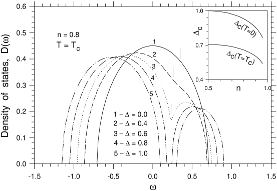
FIG. 1.: Density of states as a function of frequency for different disorder strengths $\Delta$ (in the paramagnetic phase). Vertical lines indicate the location of the chemical potential. Note that the density of states is plotted on an absolute energy scale, so the chemical potential is not shifted to lie at $\omega=0$. The inset displays the dependence of the critical values of disorder in the paramagnetic [$\Delta(T=T_{c})\equiv\Delta_{c}^{P}$] and ferromagnetic [$\Delta_{c\uparrow}(T=0)\equiv\Delta_{c}^{F}$] phases as a function of the electron filling $n$.

Figure 1 shows the influence of disorder on the conduction-electron density of states in the paramagnetic phase at $n=0.8$. When the strength of the disorder is small, the band is only slightly distorted from the semicircular shape. As the disorder increases, a pseudogap first appears and then a true gap develops when the disorder is larger than a critical value. Because the double-exchange couples ferromagnetism to the mobility of the itinerant electrons, the critical value of the disorder depends on the spin polarization of the system and on the total electron density. This is depicted in the inset to Figure 1, where the critical value of the disorder, required for the metal-insulator transition, is plotted as a function of the total electron density. Two curves are shown: (i) the critical disorder strength ($\Delta_{c}^{P}$) needed for the transition in the high-temperature paramagnetic phase $T>T_{c}$, where there is no spin polarization (bottom curve); and (ii) the critical disorder strength ($\Delta_{c}^{F}$) in the fully polarized ferromagnetic phase at $T=0$ (top curve). Since the ferromagnetic order makes the bandwidth larger, the critical value of disorder needed for the MIT increases as one enters the ferromagnetic phase. If the disorder is large enough, it is always an insulator (even in the ferromagnetic phase)—but there is a regime, where the system can be an insulator in the paramagnetic phase, and a metal in the ferromagnetic phase (at least it is metallic for the majority [spin-up] electrons, it would be insulating for the minority [spin-down] electrons). This is the regime that is relevant for the CMR materials.

In the limit where $\Delta\to\infty$, the band is always split, and the upper subband is pushed to infinite energy and can be neglected. From Eq. (32) we have

$${\rm Im}a(\omega-\mu)=\frac{1}{2}\sqrt{2t^{*2}n-\omega^{2}},\qquad\omega^{2}\leq 2t^{*2}n,$$ (34)

for $H=0$. The magnetization vanishes, because the internal molecular field $\lambda_{F}$ vanishes when $\Delta\to\infty$ as seen from Eq. (14). Hence, there is no ferromagnetic order, and the inverse of the effective medium satisfies $a_{\uparrow}(\omega)=a_{\downarrow}(\omega)=a(\omega)$. Since

$$\frac{2}{\pi t^{*2}}\int d\omega{\rm Im}a(\omega-\mu)=n,$$ (35)

for this case, the lower band is completely occupied and the chemical potential lies in the gap for all $n$.

For finite $\Delta$, the same conclusion is obtained for the high-temperature paramagnetic phase. This follows directly from the numerical calculations, but can be understood from the fact that the total spectral weight in the lower band doesn’t change until the gap closes. The ferromagnetic transition temperature generically increases from zero though. Figure 1 shows the location of the chemical potential at $T_{c}$ with vertical lines for $\Delta=0$, $\Delta=0.4$ and $\Delta=0.6$ (note that in the last case the chemical potential lies in the pseudo-gap). For $\Delta=0.8$ and $\Delta=1.0$ ($\Delta_{c}=0.6581$ at $n=0.8$), the chemical potential lies in the gap.

This situation is similar to what takes place in the static Holstein model, which is solved exactly in infinite dimensions[35, 36]. In this model, bipolaron formation leads to the opening of a gap when the electron-phonon interaction is strong enough, and the chemical potential lies in the gap for all $n$. It differs from the Mott-Hubbard transition which occurs only at half-filling.

IV Magnetic properties

The magnetism of the binary-disorder double-exchange system is determined by the uniform (ferromagnetic) magnetization

$$m=(1-n)m\Bigl{(}\frac{1}{2}\Delta\Bigr{)}+nm\Bigl{(}-\frac{1}{2}\Delta\Bigr{)},$$ (36)

and by the uniform (ferromagnetic) susceptibility

$$\chi=(1-n)\frac{dm(\frac{1}{2}\Delta)}{dh}+n\frac{dm(-\frac{1}{2}\Delta)}{dh}.$$ (37)

The algebraic equations for $dm(\Delta/2)/dh$ and $dm(-\Delta/2)/{dh}$ are taken at $h=H=m=0$ in Eq. (28) with the binary probability distribution for the disorder. The determinant of this system of equations equals zero at the ferromagnetic Curie temperature $T_{c}$.

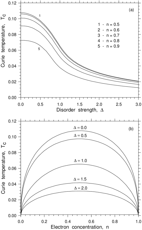
FIG. 2.: Curie temperature as a function of disorder strength $\Delta$ and electron filling $n$: (a) shows results for constant electron filling, while (b) shows results for constant disorder strength.

Figure 2 shows (a) the disorder dependence of the Curie temperature for different electron densities and (b) the electron density dependence of the Curie temperature for different disorder strengths. The value of $T_{c}$ for the pure double-exchange system [the curve $\Delta=0$ in Figure 2(b)] essentially coincides with that obtained by Furukawa for double exchange with classical local spins [12]. One needs to choose the electronic bandwidth to be quite narrow ($W$ on the order of $0.5-1$ ev for $T_{c}$ ranging from $315-630^{o}$K at $n\sim 0.5$). These estimates of $T_{c}$ for the pure double-exchange system are comparable with some materials (like LSMO where $T_{c}\sim 380^{o}$K), and are much smaller than those predicted in Ref.[6]. Nevertheless, if we take a more reasonable value for the bandwidth ($W\sim 2$ ev), then it is clear that double exchange alone cannot explain the values of $T_{c}$ for the manganites.

Figure 2 shows that disorder suppresses the ferromagnetic transition temperature. The physics of this is clear. Carrier motion promotes the double-exchange ferromagnetic order, whereas disorder reduces the electron motion, and thereby it reduces the ability of the double-exchange process to produce ferromagnetism—the net effect is to reduce $T_{c}$. The calculated disorder dependence of $T_{c}$ agrees qualitatively with that found for the combined double-exchange–Holstein model[7] and with Narimanov and Varma’s calculation[22] with a Gaussian disorder probability distribution.

Figure 2 shows also that three disorder regimes can be distinguished for our model. The first regime (renormalized double-exchange) is the regime where $T_{c}$ depends only weakly on disorder and corresponds to the flat regions of the curves in Figure  2(a) [$\Delta<0.5$]. We find that $T_{c}$ is suppressed most strongly at $0.5<\Delta<1.0$ [see Figure 2(a)]; i.e. in the vicinity of the critical values of disorder where a gap in the density of states is created. We call this regime the transition regime, where the ferromagnetism process is changing from a renormalized double-exchange process to a renormalized strong-coupling process. In this range of $\Delta$, two crossovers occur: (i) the metallic conductivity is replaced by a thermally activated (insulating) conductivity, and (ii) double-exchange ferromagnetism is replaced by a ferromagnetism that is caused by virtual electron transfers from the filled lower band to the empty upper subband (and vice versa). Indeed, the double-exchange mechanism for the ferromagnetic ordering of the local spins is caused by real electron transfers, which are possible only at small disorder. For strong disorder $(\Delta>1$), when the itinerant electrons are localized, the ferromagnetic ordering is caused by virtual transfers to neighboring sites (that have an additional local potential $\Delta$) and back. (All sites without this additional potential are filled so hopping onto those sites is impossible.) Hence, the Curie temperature is inversely proportional to $\Delta$ at strong disorder [the $1/\Delta$ behavior is clearly seen in Figure 2(a) for $\Delta>1.5$].

Usually, virtual electron transfers lead to a Heisenberg type of ferromagnetic ordering, i.e. the magnetic energy contains a $\cos{\Theta}$ dependence, not the $\cos{\Theta/2}$ dependence of double exchange. Therefore, the crossover from double-exchange ferromagnetism to disorder-induced ferromagnetism (with a Heisenberg type of magnetic energy) must be seen in the changing of the behavior of magnetic quantities (for example, paramagnetic susceptibility and magnetization) as the disorder strength increases.

In particular, an increase of the disorder strength changes the temperature dependence of the uniform susceptibility. Indeed, the pure double-exchange system ($\Delta=0$) reveals Curie-type behavior for $\chi$ at high temperatures $(\chi\sim 1/T$), i.e. the Curie temperature is equal to zero. As the temperature is decreased, the curvature of the inverse susceptibility $\chi^{-1}$ changes, so that it intersects the temperature axis at a finite temperature, yielding a nonzero value for $T_{c}$ and a Curie-Weiss law for $\chi$. This feature of double exchange was noted in the pioneering work by Anderson and Hasegawa [3] (see also Ref. [28]). (It should be noted that this aspect of double exchange is still not completely understood. See, for example, Ref. [37] where a high-temperature expansion is employed).

Numerical calculation of the uniform susceptibility, Eq. (37), at strong disorder shows that $\chi$ obeys a Curie-Weiss law with a nonzero Curie temperature in this case. Thus, the crossover to a disordered-induced mechanism of ferromagnetic ordering leads to a change in the temperature dependence of $\chi$.

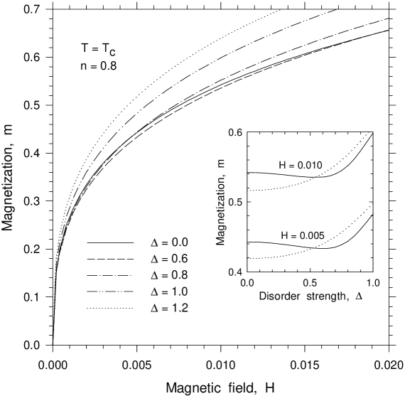
FIG. 3.: Magnetization of the local-spins $m$ as a function of the external magnetic field $H$ for different disorder strengths $\Delta$. The inset shows the disorder dependence of $m$ at $H=0.005$ and $H=0.01$ for the double-exchange model (solid lines) and for the Ising model in the mean-field approximation (dotted lines).

In Figure 3 we plot the magnetization $m$ as a function of external magnetic field $H$ at $T=T_{c}$ for a number of different disorder strengths. The field-induced magnetization at fixed magnetic field depends on disorder and the inset to Figure 3 shows that the magnetization (solid lines) initially decreases as the disorder strength increases until one reaches the region where the conduction band has a well-developed pseudogap and begins to split ($\Delta_{c}=0.6581$ for $n=0.8$). As the disorder increases further, the magnetization starts to increase and it can be described by the following mean-field equation

$$m=\tanh{\beta\Bigl{(}mT_{c}+\frac{1}{2}H\Bigr{)}},$$ (38)

for the magnetization of an Ising model (or a Heisenberg model with $S=1/2$). Dotted lines in the inset show the field-induced magnetization evaluated from (38) where $T_{c}$ is equal to the Curie temperature of the disordered double-exchange model at a given $\Delta$. Hence, the disorder dependence of the magnetization at fixed magnetic field also shows the crossover from double-exchange-induced to disorder-induced ferromagnetism at strong disorder.

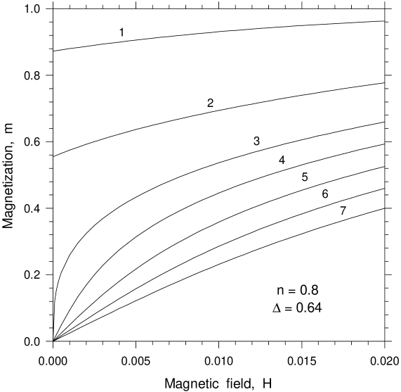
FIG. 4.: Magnetization of the local-spins, $m$, as a function of the external magnetic field $H$ for different relative temperatures $\tau=T/T_{c}$: 1 - $\tau=0.4$, 2 - $\tau=0.8$, 3 - $\tau=1.0$, 4 - $\tau=1.1$, 5 - $\tau=1.2$, 6 - $\tau=1.3$, 7 - $\tau=1.4$.

From Figure 3 we see that the most favorable conditions for a large field-induced magnetization are strong disorder and strong magnetic fields. Figure 4 shows the field dependence of $m$ for different relative temperatures $\tau=T/T_{c}$ and fixed disorder. The largest absolute value for $m$ is observed at small $\tau$ ($\tau=0.4$) but the relative increase of $m$ (when $H$ is also increased) is weak. The strongest growth of $m$ at weak fields is seen near the Curie temperature. At $T=T_{c}$ ($\tau=1.0$) this growth is maximal, but even at $\tau=1.4$ the $H$ dependence of $m$ is linear. Note that such behavior of the field-induced magnetization is in good agreement with the experimental data on the manganites [14].

Our analysis of the magnetic properties has shown the emergence of three different regimes: (i) a renormalized double-exchange regime (or weak-disorder regime); (ii) a strong-coupling physics regime (or strong-disorder regime); and (iii) a transition regime where the properties crossover from metal to insulator and from double-exchange ferromagnetic ordering to strong-coupling-induced ferromagnetism. This classification scheme will be more sharply defined as we examine the transport properties in Section V.

V Transport properties

In this section, we consider the electrical and thermal transport properties of the double-exchange system in zero external magnetic field. The transport is determined from the following set of equations[38]. The electrical conductivity $\sigma=1/\rho$ is

$$\sigma=L_{11};$$ (39)

the thermopower is

$$S=-\frac{k_{B}}{|e|}\frac{1}{T}\frac{L_{12}}{L_{11}},\qquad\frac{k_{B}}{|e|}\simeq 86\mu\mbox{VK${}^{-1}$};$$ (40)

and the thermal conductivity (of the electronic system) satisfies

$$\kappa=\biggl{(}\frac{k_{B}}{e}\biggr{)}^{2}\frac{1}{T}\Bigl{\{}L_{22}-\frac{L_{12}^{2}}{L_{11}}\Bigr{\}};$$ (41)

where the transport coefficients $L_{ij}$ are defined by

$$L_{ij} = \pi\sigma_{0}\sum_{\sigma}\int\limits_{-\infty}^{\infty}d\varepsilon v^{2}(\varepsilon)D^{0}(\varepsilon)$$ (42)

$$\int\limits_{-\infty}^{\infty} d\omega\biggl{(}-\frac{df(\omega)}{d\omega}\biggr{)}(\omega-\mu)^{i+j-2}A^{2}_{\sigma}(\varepsilon,\omega-\mu).$$ (43)

Here the spectral function is given by

$$A_{\sigma}(\varepsilon,\omega)=-\frac{1}{\pi}\mbox{Im}{\cal G}_{\sigma}(\varepsilon,\omega),$$ (44)

$\sigma_{0}$ is the unit of conductivity, ${\cal G}_{\sigma}(\varepsilon,\omega)$ is given in Eq. (17) and $v(\varepsilon)$ is the current vertex which is equal to

$$\sqrt{(4t^{*2}-\varepsilon^{2})/3},$$ (45)

for the Bethe lattice[39, 40] with $z\to\infty$.

Figure 5 shows the temperature dependence of the resistivity for different electron fillings in the three different disorder regimes. (In this and the following Figures, the resistivity is plotted in units of $\rho_{0}=1/\sigma_{0}$). In Figure 5(a), the weak-disorder regime, the transport properties are determined by the double-exchange mechanism. From Eqs. (21) and (32), one obtains the following expression for the electronic self-energy

$$\Sigma_{\sigma}(\omega+i\delta)=-\frac{1}{2}\biggl{(}\frac{1-\sigma m}{1+\sigma m}\biggr{)}$$

$$\times\Bigl{\{}\omega+\mu\pm\sqrt{(\omega+\mu)^{2}-2t^{*2}(1+\sigma m)}\Bigr{\}},$$ (46)

at $\Delta=0$. Therefore,

$${\rm Im}\Sigma_{\sigma}(\omega+i\delta)=-\frac{1}{2}\biggl{(}\frac{1-\sigma m}{1+\sigma m}\biggr{)}$$

$$\times\sqrt{2t^{*2}(1+\sigma m)-(\omega+\mu)^{2}},$$ (47)

for $(\omega+\mu)^{2}\leq 2t^{*2}(1+\sigma m)$ and $\mbox{Im}\Sigma_{\sigma}(\omega+i\delta)=0$ otherwise.

Note that the factor

$$\frac{1-\sigma m}{1+\sigma m},$$ (48)

in Eq. (47) is contained in the expression for the self-energy in Ref.[41] for the pure double-exchange system with classical local spins and a Lorentzian density of states (we use a semicircular density of states here). This factor plays an essential role in the low-temperature behavior of the resistivity [Figure 5(a)]. It provides a decrease in the resistivity when the magnetization increases. Indeed, in the limit $m\to 1$ or $T\to 0$, we have

$$A_{\uparrow}(\varepsilon,\omega)=\delta(\omega+\mu-\varepsilon),\qquad A_{\downarrow}(\varepsilon,\omega)=0,$$ (49)

and the conduction-electron subsystem becomes a free-electron gas of spin-up electrons with a conductivity that is a delta function at zero frequency (whose strength is the Drude weight).

On the other hand, in the high-temperature paramagnetic phase, $m=0$, and the correlated bandwidth is narrowed by a factor of $\sqrt{2}$ due to paramagnetic spin disorder. In this case, the expression for the self-energy exactly coincides with the one obtained in Ref. [7] for the pure double-exchange system. Since the density of states is independent of temperature here, all of the temperature dependence of the resistivity arises from the Fermi factor $[-df(\omega)/d\omega]$ [see Eq. (43)]. If one makes the assumption that the chemical potential is also temperature-independent, so that the derivative of the Fermi factor depends only weakly on temperature, then one would conclude[12, 22] that the resistivity in the paramagnetic phase (due to double exchange only) is essentially a constant. However, more accurate calculations, that take into account the temperature dependence of the chemical potential, show that the pure double-exchange system becomes a bad-metal with $d\rho/dT>0$ [see, for example, Ref. [7] where the bad-metal behavior was shown in a double-exchange system with weak electron-phonon interaction in their Figure 6(a)].

The sharp decrease of the resistivity at $T<T_{c}$ for all $n$ is caused by the rapid increase of the magnetization $m$. This discontinuity in the slope $d\rho/dT$ at $T=T_{c}$ is a consequence of the dynamical mean-field approach. Incorporation of spatial spin fluctuations[27] will smooth out the temperature dependence of the resistivity in the vicinity of $T_{c}$, but this is beyond dynamical mean field theory.

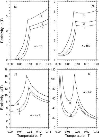
FIG. 5.: Temperature dependence of the resistivity $\rho$ for different disorder strengths $\Delta$: (a) $\Delta=0$, (b) $\Delta=0.5$, (c) $\Delta=0.75$ and (d) $\Delta=1.0$. The curves labeled by 1 correspond to an electron filling of $n=0.6$; 2 denotes $n=0.7$; and 3 denotes $n=0.8$.

As disorder is added to the system, the properties are initially changed little. When the disorder becomes large enough $\Delta\approx 0.4$, then we start to feel a more direct influence of the disorder as it produces a pseudogap in the density of states and we enter the transition regime of moderate disorder. In this regime, the slope of the resistivity can become negative $d\rho/dT$ above $T_{c}$ as shown in Figures 5(b) and 5(c). The value $\Delta\simeq 0.4$ is the boundary value that separates the weak-disorder and the moderate-disorder regimes for $n=0.8$. As the disorder is increased further, the metallic conductivity is gradually replaced by a thermally activated conductivity (this starts at $\Delta\approx\Delta_{c}^{P}$). As one enters the strong-disorder regime, there is a MIT at $T_{c}$. Here the system displays insulating behavior everywhere, except just below the Curie point, where the rapid increase in the magnetization can cause the resistance to drop over a small temperature range before it turns around and increases again. This occurs in the transition from the paramagnetic insulator to the ferromagnetic insulator because the charge gap in the ferromagnetic insulator is smaller than the charge gap in the paramagnetic insulator. Those sharp cusps seen in Figure 5(d) will generically be smoothed out by spatial fluctuations.

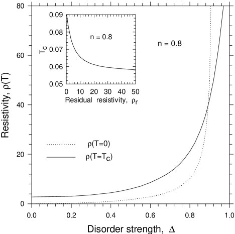
FIG. 6.: Resistivity at $T=0$ (dotted line) and at $T=T_{c}$ (solid line) versus disorder strength. Inset is a plot of the Curie temperature $T_{c}$ versus the residual resistivity $\rho_{r}=\rho(T=0)$. Note how the two resistivity curves cross at a critical value of disorder, which determines the beginning of the transition region from the moderate to strong-disorder regimes.

We can analyze the transition from moderate to strong disorder more quantitatively. We focus on two characteristic resistivities: the resistivity at $T_{c}$ and the resistivity at $T=0$ (residual resistivity). For weak disorder the residual resistivity is much smaller than the resistivity at $T_{c}$. When we reach the moderate disorder regime, the residual resistivity starts to increase rapidly, eventually overtaking the resistivity at $T_{c}$ in the strong-disorder regime. We denote the boundary between the moderate and strong-disorder regimes by the value of disorder where $\rho(T=0)=\rho(T=T_{c})$. This occurs at $\Delta\simeq 0.892$ for $n=0.8$ as shown in Figure 6. This transition occurs when the density of states has developed a strong pseudogap, but has not yet become an insulator ($\Delta_{c}^{F}=0.931$ for $n=0.8$). The range of disorder between these two limits, ($0.892<\Delta<\Delta_{c}^{F}=0.931$ for $n=0.8$) is the transitional region between the moderate-disorder and the strong-disorder regimes.

This analysis is in qualitative agreement with the calculations that use a Lorentzian density of states[23] and especially with calculations[18] that show a divergence of the $T=0$ resistivity at a critical disorder strength. Note that Anderson localization is the cause of the MIT in Ref. [18].

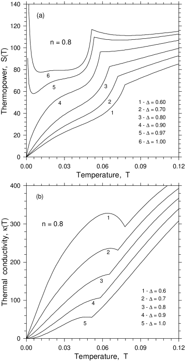
FIG. 7.: Temperature dependence of (a) the thermopower and (b) the electronic thermal conductivity for different values of disorder.

The inset to Figure 6 shows the Curie temperature as a function of the residual resistivity $\rho(T=0)$. This plot was obtained by combining the $\Delta$ dependences of $\rho(T=0)$ and $T_{c}$ (see Figure 2). It is clearly seen that the suppression of $T_{c}$ due to disorder is accompanied by the increase of the residual resistivity. We find that our functional dependence of $T_{c}$ on $\rho(T=0)$ is smoother than that found in Ref. [18] and agrees better with experiment [18, 42].

Now we examine the thermal properties of our system including the thermopower $S(T)$ and the electronic thermal conductivity $\kappa(T)$ which are shown in Figure 7. The behavior of these two quantities are quite different from each other—while the thermal conductivity always vanishes as $T\to 0$, the thermopower will either vanish or diverge depending on whether the system is metallic or insulating as $T\to 0$. The thermal conductivity behaves as expected with a sharp increase at $T_{c}$ due to the opening of conduction channels as the magnetization grows, and a linear decrease to zero at low temperatures. Note that the thermal conductivity vanishes at low temperatures even in the metal, because the heat current vanishes.

The thermopower behaves quite a bit differently. It too shows a strong effect at $T_{c}$ (in this case a sharp decrease), but the low temperature behavior is most interesting. For weak disorder (metallic phases), the thermopower vanishes as $T\to 0$, but once a gap opens in the density of states, the thermopower diverges as $T\to 0$ since the chemical potential lies in the gap. Peltier’s coefficient, $P=TS(T)$, is approximately given by a straight line for strong disorder ($\Delta=1.0$) and low temperature (where the magnetization has saturated $m\simeq 1$), i.e. $P=\alpha+\gamma T,$ $\alpha\simeq 0.17\mu$V. Hence, the thermopower $S(T)$ can be approximately represented by

$$S(T)\simeq\frac{\alpha}{T}+\gamma,$$ (50)

for low temperature and strong disorder. This relation is typical of what is seen in intrinsic semiconductors [43] Note that the thermopower behaves similarly for electronic systems that undergo Anderson localization[44]: if the chemical potential is in the region of localized states, then $S(T)$ also diverges as $T\to 0$.

The slope of the thermopower $dS/dT$ has a discontinuity at $T_{c}$, but $S(T)$ does not change sign in our model. The prediction[45] that $S(T)$ alter its sign at $T=T_{c}$ in double-exchange systems was founded on two principles: (i) the itinerant-electron subsystem is a Fermi-liquid and (ii) the derivative of the chemical potential $d\mu/dT$ changes sign at $T=T_{c}$. While we find that the derivative $d\mu/dT$ does change sign at $T=T_{c}$ in agreement with others[12, 28], the itinerant-electron subsystem is not a Fermi-liquid in our model, because the imaginary part of the self-energy does not vanish as $T\to 0$ at the Fermi-energy. Hence, the reasoning that led to the prediction of a sign change cannot be applied here.

The high-temperature behavior of the thermopower for strong disorder is similar to that of $S(T)$ in a small-polaron model[46] where the conductivity is thermally activated and $S(T)\sim\ln[{c/(1-c)}]$; with $c$ the small-polaron concentration and $c\leq 1$. Indeed, the thermopower has a weak temperature dependence for strong disorder [see Figure 8(a)] in the paramagnetic phase and $T\gg T_{c}$. Furthermore, for fixed temperature, we find that $S(T)$ decreases when the electron filling is decreased to $n=0.5$. At $n=0.5$ the thermopower is equal to zero at all temperatures as in the small-polaron theory. Below $n=0.5$, we find that the thermopower changes sign. Hence we only find a sign change of the thermopower when the electron filling is varied.

VI Magnetoresistance

The most interesting property of the manganites is the fact that the resistance changes so dramatically in a magnetic field. This makes them useful as possible magnetic field sensors for the magnetic storage community. We find similar magnetoresistance effects in our model, especially when we are close to the Curie point. The origin of the magnetoresistance lies in the sensitivity of the resistivity to the magnetization, and the ease with which $m$ can be tuned by a magnetic field. Typically, the field increases $m$, which then reduces the resistivity. Experimentally[14], there is a strong correlation between the field-induced changes in $\rho$ and $m$.

In order to calculate the magnetoresistance, we must first solve for the conductivity in the presence of an external magnetic field. If we perform a simple shift in the definition of the inverse effective medium $a_{n\sigma}\to a_{n\sigma}+H\sigma/2$ and replace the integration variable in Eq. (32) by $\omega\to\omega+H\sigma/2$, then the only modification is that the derivative of the Fermi factor $[-df(\omega)/d\omega]$ now has an explicit $H$ dependence and the spectral function $A_{\sigma}$ in Eq. (34) depends on $H$ through the magnetization $m$. The direct dependence of $\rho$ on $H$ via the factor $[-df(\omega)/d\omega]$ always yields a small positive magnetoresistance that is caused by the Zeeman interaction with the external magnetic field; it can be neglected in weak fields.

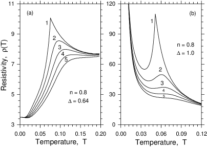
FIG. 8.: Temperature dependence of the resistivity $\rho(T)$ for different magnetic fields $H$: 1 - $H=0.0$, 2 - $H=0.005$, 3 - $H=0.01$, 4 - $H=0.015$, 5 - $H=0.02$.

Figure 8 shows the temperature dependence of the resistivity for different magnetic fields and two disorder regimes: (a) moderate-disorder and (b) strong-disorder. The field-induced modifications to the magnetization suppress the resistivity. This effect is strongest in the vicinity of the Curie point, because the spin susceptibility is large there; hence the field changes the magnetization most strongly there. The peak position in $\rho(T)$ shifts to higher temperature with increasing $H$ and there is a critical value of $H$ above of which the MIT disappears (i.e., $d\rho/dT>0$ for all temperatures). This picture qualitatively agrees with the experimental data on manganites [1, 14].

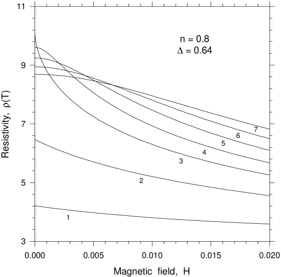
FIG. 9.: Resistivity $\rho(T)$ as a function of external magnetic field $H$ for different relative temperatures $\tau=T/T_{c}$: 1- $\tau=0.4$, 2 - $\tau=0.8$, 3 - $\tau=1.0$, 4 - $\tau=1.1$, 5 - $\tau=1.2$, 6 - $\tau=1.3$ and 7 - $\tau=1.4$.

The magnetic-field dependence of the resistivity at different relative temperatures $\tau=T/T_{c}$ (Figure 9) also indicates the close correlation between the field-induced changes in $\rho$ and $m$. Indeed, the comparison of Figures 4 and 9 shows that the magnitude of resistivity correlates with the change in the magnetization: the suppression of the resistivity is large around $T_{c}$ where the largest growth of $m$ is seen (see Figure 4) but is weak far below and above $T_{c}$. Our calculation of the $H$ dependence of $\rho$ is in good qualitative agreement with experiment (see Figure 7 in Ref. [14]).

We define the magnitude of the relative magnetoresistance as

$$\frac{\delta\rho}{\rho}=\frac{\rho(T,0)-\rho(T,H)}{\rho(T,0)}.$$ (51)

In this definition, $\delta\rho/\rho$ is positive and cannot exceed 100%. Figure 10 shows the magnetoresistance as (a) a function of $H$ and (b) as a function of $m^{2}$ for different disorder strengths at $T=T_{c}$. It is seen from the comparison of Figure 3 and Figure 10(a) that the field-dependence of the magnetization is directly reflected in the field-dependence of the magnetoresistance. The $\Delta$ dependence of $\delta\rho/\rho$ at fixed $H$ is shown in the inset to the Figure 10(a). The comparison of this inset with the inset to Figure 3 shows that disorder dependences of $\delta\rho/\rho$ and $m$ at fixed $H$ are also similar. In the weak-disorder regime, $\delta\rho/\rho$ is slightly decreased. Although the double-exchange mechanism of ferromagnetic ordering becomes weaker in this regime, it is still active. In the moderate-disorder regime, strong-coupling-induced ferromagnetism (discussed in Section IV) replaces the double exchange, and the magnetization begins to increase with increasing disorder. This leads to an increase of the magnetoresistance for both the moderate-disorder and strong-disorder regimes. At $\Delta=1.0$, $\delta\rho/\rho$ can attain values near 70% in a weak field of $H=0.01$.

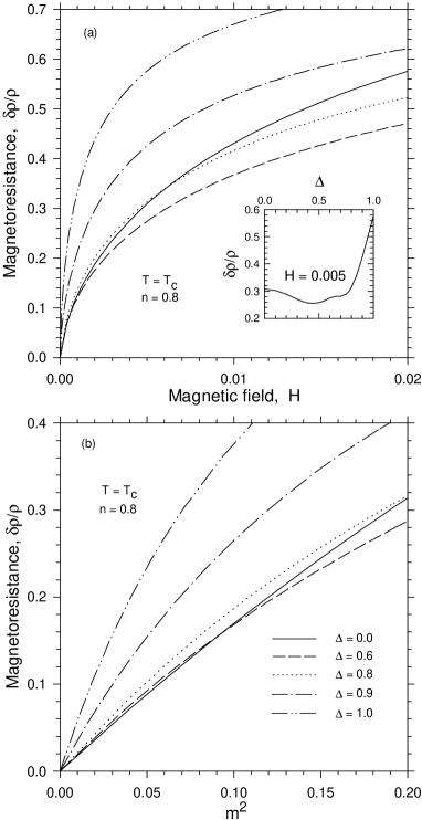
FIG. 10.: (a) Magnetoresistance $\delta\rho/\rho$ as a function of the external magnetic field $H$ and (b) magnetoresistance as a function of $m^{2}$ for different disorder strengths. The inset shows the disorder-dependence of $\delta\rho/\rho$ for $H=0.005$. The line styles in (a) are the same as in (b).

Figure 10(b) shows that the magnetoresistance can be expressed by a scaling law

$$\frac{\delta\rho}{\rho}=Cm^{2},$$ (52)

where the scaling constant $C$ is independent of $T$ only for the pure double-exchange system ($\Delta=0$). The relation (52) is approximately satisfied for finite disorder $0\leq\Delta\leq 1.0$ (at least for $m^{2}<0.01$), but the coefficient $C$ is rather high, about 4, for $\Delta=1.0$ ($n=0.8$). versus its value of 1.9 for weak-to-moderate-disorder $(0<\Delta<0.6)$. Note that Furukawa’s calculation [47] performed for the pure-double exchange system with classical local spins gives the value of 4 for $C$ (when $n$ is also equal to 0.8). The difference between our estimate of $C$ and Furukawa’s arises from the different density of states. Note that Kubo and Ohata [5] obtain $C=1$ for the quantum double-exchange system. The scaling constant $C$ also depends on band filling. $C$ decreases with decreasing electron filling. In particular, $C=1.7$ $(\Delta=0)$ and $C=2.5~{}(\Delta=1.0)$ for $n=0.67$. Thus, we can conclude that the band filling near $n=0.8$ and relatively strong disorder ($\Delta>0.9$) are the most favorable conditions for a large magnetoresistance.

VII Conclusion

We have considered the influence of diagonal disorder on a simple double-exchange model with local Ising spins by employing dynamical mean-field theory. We choose a binary probability distribution for the disorder which greatly simplified the analysis and allowed us to examine directly the MIT. The manganites are too complicated a system to be described completely by this simple model. Nevertheless, we still arrive at some useful conclusions: (i) double exchange alone cannot explain the metal-insulator transition in manganites (in the best case, it can be applicable to LSMO at $x\simeq 0.3$ which has a relatively high Curie temperature and displays bad-metal behavior in the paramagnetic phase); (ii) double exchange plus disorder cannot explain the temperature dependence of the thermopower $S(T)$ because it does not yield a change of sign in the paramagnetic phase. An explanation of the large peak in $S(T)$ (in the ferromagnetic phase) is beyond dynamical mean field theory, because it does not include magnon drag[48]; (iii) the effect of diagonal disorder (induced by chemical substitution) is important, and can influence the properties of the material if the disorder strength is large enough to be close to the MIT; and (iv) we identified three disorder regimes which display different characteristic behavior. The weak-disorder regime has little effect on the system and just renormalizes the double-exchange mechanism of ferromagnetic ordering. The moderate-disorder regime, corresponds to the transition region between weak and strong disorder. The interacting density of states develops a pseudogap that promotes behavior similar to thermal activation. The double-exchange mechanism is gradually replaced by a strong-coupling ferromagnetism (see Section IV) which has a mean-field-like magnetism. In this regime, the Curie temperature is sharply decreased and the temperature dependence of the resistivity reveals a MIT at $T=T_{c}$. The strong-disorder regime, is characterized by a gap in the interacting density of states at high temperature and the residual resistivity exceeds the resistivity at $T=T_{c}$. Ferromagnetic ordering of local spins (with small values of $T_{c}\sim 1/\Delta$) occurs due to strong-coupling physics. This regime is most favorable to obtain a large magnetoresistance.

- [1] For a review see A. P. Ramirez, J. Phys.: Condens. Matter 9, 8171 (1997).
- [2] P. W. Anderson and H. Hasegawa, Phys. Rev. 100, 675 (1955).
- [3] C. Zener, Phys. Rev. 82, 403 (1951).
- [4] P.-G. de Gennes, Phys. Rev. 118, 141 (1960).
- [5] K. Kubo and N. Ohata, J. Phys. Soc. Japan 33, 221 (1972).
- [6] A. J. Millis, P. B. Littlewood and B. I. Shraiman, Phys. Rev. Lett. 74, 5144 (1995).
- [7] A. J. Millis, R. Mueller and B. I. Shraiman, Phys. Rev. B 54, 5405 (1996).
- [8] H. Röder, J. Zang and A. R. Bishop, Phys. Rev. B 53, R8840 (1996).
- [9] A. S. Alexandrov and A. M. Bratkovsky, Phys. Rev. Lett. 82, 141 (1999).
- [10] A. C. M. Green, cond-mat/002297; A.C.M. Green and D.M. Edwards, Physica B 281-282, 534 (2000); D.M. Edwards, A.C.M. Green, and K. Kubo, Physica B 259-261, 810 (1999); J. Phys.: Condens. Matter 11, 2791 (1999).
- [11] C. M. Varma, Phys. Rev. B 54, 7308 (1996).
- [12] N. Furukawa, in Physics of Manganites, edited by T. A. Kaplan and S. D. Mahanti, (New York, Kluwer/Plenum, 1999).
- [13] S. K. Sarker, J. Phys.: Condens. Matter 8, 1515 (1996).
- [14] A. Urushibara, Y. Morimoto, T. Arima, A. Asamitsu, G. Kido and Y. Tokura, Phys. Rev. B 51, 14103 (1995).
- [15] S. H. Chun, M. B. Salamon, Y. Tomioka and Y. Tokura, Phys. Rev. B 61, R9225 (2000).
- [16] Y. Lyanda- Geller, S. H. Chun, M. B. Salamon, P. M. Goldbart, P. D. Han, Y. Tomioka, A. Asamitsu and Y. Tokura, cond-mat/0012462.
- [17] Q. Li, J. Zang, A. R. Bishop and C. M. Soukoulis, Phys. Rev. B 56, 4541 (1996).
- [18] L. Sheng, D. Y. Xing, D. N. Sheng and C. S. Ting, Phys. Rev. B 56, R7053 (1997).
- [19] L. Sheng, D. Y. Xing, D. N. Sheng and C. S. Ting, Phys. Rev. Lett. 79, 1710 (1997).
- [20] N. G. Bebenin, R. I Zainullina, V. V. Mashkautsan, V. S. Gaviko, V. V. Ustinov, Ya. M. Mukovskii and D. A. Shulyatev, Zh. Eks. Teor. Fiz. 117, 1181 (2000) [Sov. Phys. JETP 90, 1027 (2000)].
- [21] F. Zhong, J. Dong and Z. D. Wang, Phys. Rev. B 58, 15310 (1998).
- [22] E. E. Narimanov and C. M. Varma, cond-mat/0002191.
- [23] M. Auslender and E. Kogan, cond-mat/0006184.
- [24] I. M. Lifshitz, Sov. Phys. Usp. 7, 549 (1964).
- [25] M. S. Laad, L. Craco and E. Müller-Hartmann, cond-mat/9911378.
- [26] V. N. Smolyaninova, X. C. Xie, F. C. Zhang, M. Rajeswari, R. L. Greene and S. Das Sarma, Phys. Rev. B 62, 3010 (2000).
- [27] S. Ishizaka and S. Ishihara, Phys. Rev. B 59, R8375 (1999).
- [28] B. M. Letfulov, Eur. Phys. J. B 4, 195 (1998); B 14, 19 (2000).
- [29] B. Vlaming and D. Vollhardt, Phys. Rev. B 45, 4637 (1992).
- [30] L.M. Falicov and J.C. Kimball, Phys. Rev. Lett. 22, 997 (1969).
- [31] U. Brandt and C. Mielsch, Z. Phys. B 75, 365 (1989); ibid. 79, 295 (1990); U. Brandt, A. Fledderjohann, and G. Hülsenbeck, ibid. 81, 409 (1990); U. Brandt and A. Fledderjohann, ibid. 87, 111 (1992); J.K. Freericks and V. Zlatić, Phys. Rev. B 58, 322 (1998).
- [32] V. Jaňis and D. Vollhardt, Phys. Rev. B 46, 15712 (1992).
- [33] J. H. Park, C. T. Chen, S.-W. Cheong, W. Bao, G. Meigs, V. Chakarian and Y. U. Idzerda, Phys. Rev. Lett. 76, 4215 (1996).
- [34] P.G.J. Van Dongen, Phys. Rev. B 45, 2267 (1992); P.G.J. Van Dongen and C. Leinung, Ann. Phys. (Leipzig) 6, 45 (1997).
- [35] J.K. Freericks, M. Jarrell and D. J. Scalapino, Phys. Rev. B 48, 6302 (1993).
- [36] A. J. Millis, R. Mueller and B. I. Shraiman, Phys. Rev. B 54, 5389 (1996).
- [37] H. Röder, R. R. P. Singh and J. Zang, Phys. Rev. B 56, 5084 (1997).
- [38] M. Jonson and G.D. Mahan, Phys. Rev. B 21, 4223 (1980); ibid. 42, 9350 (1990); Th. Pruschke, M. Jarrell and J. K. Freericks, Adv. Phys. 44, 187 (1995); G.D. Mahan and J.O. Sofo, Proc. Natl. Acad. Sci. 93, 7436 (1996); G.D. Mahan, Sol. State Phys. 51, 81 (1998).
- [39] W. Chung and J.K. Freericks, Phys. Rev. B 57, 11955 (1998).
- [40] A. Chattopadhyay, A. J. Millis and S. Das Sarma, Phys. Rev. B 61, 10738 (2000).
- [41] N. Furukawa, J. Phys. Soc. Japan 64, 2734 (1994).
- [42] J. M. D. Coey, M. Viret, L. Ranno and K. Ounadjela, Phys. Rev. Lett. 75, 3910 (1995).
- [43] N. F. Mott and E. A. Davis, Electronic Processes in Non-Crystalline Materials, (London and New York, Oxford University Press, 1971).
- [44] C. Villagonzalo and R. Römer, Ann. Phys. (Leipzig) 7, 394 (1998); C. Villagonzalo, R. Römer, and M. Schreiber, Eur. Phys. J. (France) B 12, 179 (1999).
- [45] D. P. Arovas, G. Gomes-Santos and F. Guinea, Phys. Rev. B 59, 13569 (1999).
- [46] G. Mahan, Many-Particle Physics (New York and London, Plenum, 1981), Chapter 7.
- [47] N. Furukawa, J. Phys. Soc. Japan 63, 3214 (1994).
- [48] P. Mandal, Phys. Rev. B 61, 14675 (2000).