ARPES Line Shapes in FL and non-FL Quasi-Low-Dimensional Inorganic Metals

Abstract

Quasi-low-dimensional (quasi-low-D) inorganic materials are not only ideally suited for angle resolved photoemission spectroscopy (ARPES) but also they offer a rich ground for studying key concepts for the emerging paradigm of non-Fermi liquid (non-FL) physics. In this article, we discuss the ARPES technique applied to three quasi-low-D inorganic metals: a paradigm Fermi liquid (FL) material TiTe₂, a well-known quasi-1D charge density wave (CDW) material K_0.3MoO₃ and a quasi-1D non-CDW material Li_0.9Mo₆O₁₇. With TiTe₂, we establish that a many body theoretical interpretation of the ARPES line shape is possible. We also address the fundamental question of how to accurately determine the k_F value from ARPES. Both K_0.3MoO₃ and Li_0.9Mo₆O₁₇ show quasi-1D electronic structures with non-FL line shapes. A CDW gap opening is observed for K_0.3MoO₃, whereas no gap is observed for Li_0.9Mo₆O₁₇. We show, however, that the standard CDW theory, even with strong fluctuations, is not sufficient to describe the non-FL line shapes of K_0.3MoO₃. We argue that a Luttinger liquid (LL) model is relevant for both bronzes, but also point out difficulties encountered in comparing data with theory. We interpret this situation to mean that a more complete and realistic theory is necessary to understand these data.

Keywords: Angle resolved photoemission line shape; Fermi liquid; Luttinger liquid; Charge density wave

1 Introduction

Angle resolved photoemission spectroscopy (ARPES) is one of the most direct probes of the electronic structure of solids. By directly measuring single-particle excitation spectra as a function of momentum and energy, it can determine the most basic quantities of condensed matter physics, e.g. the band structure, Fermi surface (FS) and electronic gap opening. Furthermore, the (AR)PES line shape can give crucial information about important ground state properties as discussed in other articles in this volume. For technical reasons, ARPES is especially well suited to quasi-2-dimensional (quasi-2D) and quasi-1D layered materials in which the electron dispersion perpendicular to the cleavage surface is small. In this case, it becomes simpler to interpret ARPES because one is primarily concerned with momenta parallel to the surface which are conserved quantities in the photoemission process and because the photohole line shape is free from the finite photoelectron lifetime induced momentum averaging effect [1, 2], which can severely limit the momentum resolution along the surface normal direction and give an added broadening of the line shape.

Quasi-low-D materials are interesting because interacting 1D systems are fundamentally different from interacting 3D systems. In 3D, the Landau Fermi liquid (FL) theory [3, 4] is a well-accepted paradigm. In this theory, a system of strongly interacting electrons (and holes) is viewed as that of weakly interacting quasi-particles with enhanced masses. In 1D, a FL is completely unstable. First, forward scatterings between electrons give rise to a Luttinger liquid (LL) [5], in which a quasi-particle no longer exists and spin and charge collective excitations completely describe the low energy physics. We will discuss the LL further in Section 5. Second, backward scattering of an electron from one FS to the other leads to spontaneous charge density wave (CDW) formation [6], which opens up a gap at $E_{F}$, making the material become an insulator [7]. The standard CDW model is the Frölich model [8]. The mean field solution of this model is formally equivalent to the BCS solution for superconductivity. However, in a quasi-1D system, fluctuation effects are expected to be very important and, e.g. lead to a pseudo-gap in the normal state. We will discuss the CDW theory further in Section 6.

Lately, interest in low-D physics seems to be expanding rapidly, partly due to high interest in low-D artificial structures and nano-scale materials. However, at this stage, it may be said that a proper understanding of real low-D materials is lacking. For example, high temperature superconductors show behaviors in photoemission, e.g. pseudo-gaps [9, 10], signs of critical fluctuations [11] and strange normal state line shapes [12], which are clearly not understood within the standard BCS theory and which still await a coherent explanation. Similarly, CDW materials, such as the blue bronze [13] and TTF-TCNQ [14] show anomalies that are not reconcilable within the standard mean-field Frölich model. In studying quasi-1D materials, it seems a necessity to learn the importance of the two phenomena inherent to 1D – the CDW and the LL. Note also that a real system is never strictly 1D but always has residual 3D couplings between chains. Therefore, a proper understanding of 3D couplings is also important. In fact, one may say that 3D couplings are essential to understand quasi-1D materials, because (1) a finite $T$ CDW transition is possible only because of them, and (2) interacting electrons strictly in 1D form a Wigner lattice [15] instead of the LL, due to unscreened long range Coulomb interaction.

In this article, we show how ARPES data let us confront these difficult but fascinating issues. Especially using a state of the art high resolution spectrometer such confrontations become more revealing than previously. We discuss three systems, a FL reference TiTe₂, a quasi-1D non-CDW, the "Li purple bronze" Li_0.9Mo₆O₁₇, and a quasi-1D CDW, the "blue bronze" K_0.3MoO₃. These three materials represent three quite different categories but, like the high temperature superconductor (HTSC) Bi2212, all are inorganic layered 3D crystals for which large samples are available. Such materials are high on the priority list for ARPES studies. Cleaving yields high quality surfaces of large area which are more stable for ARPES than those of many organic low-D conductors. Thus it is easier to obtain reproducible bulk-representative ARPES data. Also conventional thermal and transport data are readily available to be correlated with the ARPES data. Meeting all these prerequisites simultaneously is often difficult for other kinds of low-D materials.

This paper is organized as follows. Section 2 describes the theoretical background for ARPES and Section 3 summarizes experimental conditions. Section 4 describes the FL interpretation of ARPES data for the Ti $3d$ band of TiTe₂. The special property of the Ti $3d$ band that its Fermi velocity ($v_{F}$) is small leads to a quite unusual situation in which the ARPES dispersion moves across the chemical potential, $\mu$. We report such data and compare the $\mathbf{k}_{F}$ value determined from it with values estimated by other methods used by ARPES practitioners. Section 5 describes the photoemission data of Li_0.9MoO₁₇ and Section 6 describes the photoemission data of K_0.3MoO₃. We report the absence in Li_0.9MoO₁₇ and the presence in K_0.3MoO₃ of a gap opening associated with their phase transitions. We discuss non-FL line shapes found for these materials in view of currently available LL and CDW theories.

2 Theoretical Framework

Within the sudden approximation [16], the ARPES line shape is described, up to a matrix element factor, as

$$I(\mathbf{k},\omega,T)=\sum_{\omega^{\prime}}f(\omega^{\prime},T)\,\sum_{\mathbf{k}^{\prime}}A(\mathbf{k}^{\prime},\omega^{\prime},T)$$ (1)

where $f$ is the Fermi-Dirac distribution function, $A$ is the single particle spectral function and $T$ is temperature. Sums over $\mathbf{k}^{\prime}$ and $\omega^{\prime}$ account for the momentum and energy resolutions of the instrument, respectively, with resolution functions implied in the summation notation for simplicity. The energy resolution function can be obtained from the Fermi edge of a reference sample (polycrystalline Ag, Au or Pt) and, in our case, is found to be a gaussian function to a good approximation. The momentum resolution function can be modeled based on geometrical considerations. For our cases, where the band dispersion is dominant along one direction, it can be modeled as a gaussian sum over momentum along that direction.

In order to understand the ARPES line shape, it is quite useful to mentally process Eq. (1) from right to left. The final step – convolution in $\omega^{\prime}$ – is not important for a qualitative understanding, because its effect is “just” energy broadening. The most important part in Eq. (1) is the spectral function $A$, which is by definition $\mathrm{Im}\,G/\pi$, where $G$ is the single particle Green’s function. Often, $G$ is written as $1/(\omega-\epsilon(\mathbf{k})-\Sigma(\mathbf{k},\omega))$ where $\epsilon(\mathbf{k})$ is the one-electron band energy for momentum $\mathbf{k}$ and $\Sigma(\mathbf{k},\omega)$ is the so-called self energy, which contains all the information about the single-particle interaction physics of the system.

There are other general effects that we do not consider in this article. First, an additional sum over momentum along the surface normal direction, $\mathbf{k}_{\perp}$, must be included to account for the finite photo-electron lifetime [1]. This effect is minimized for quasi-low-D materials, as already noted in the previous section, because then $A$ is not dependent on $\mathbf{k}_{\perp}$ to a first approximation. An estimate of an upper-bound for the line broadening due to this effect can be made for each of our materials, as is done for TiTe₂ [17], and confirms that this effect can be safely neglected. Another effect is the inelastic background [18]. In general, this is quite difficult to quantify for ARPES, and remains an important issue especially for the HTSC’s [19]. In the next section, we will see that the TiTe₂ data show an extremely low background. We take this to imply the likelihood that the inelastic background is very small within $\sim 1$ eV from the chemical potential $\mu$ for ARPES data taken with photon energy $\sim 20$ eV on good cleaved surfaces of other samples as well.

3 Experimental Setup

ARPES data reported in this article were obtained at the Wisconsin Synchrotron Radiation Center (SRC). ARPES data were taken at the Ames/Montana beamline with a 50 mm radius VSW analyzer having a $\pm 1^{o}$ angle acceptance cone. ARPES data with angle resolution $\pm 0.18^{o}$ along the main band dispersion axis were obtained at the 4m NIM line or the PGM line with a Scienta SES 200 analyzer. Angle integrated PES data were obtained with a VG ESCALAB Mk II spectrometer ($\pm 12^{o}$ angle acceptance cone) in the home lab or with the Scienta SES 200 analyzer in the angle integrated mode (angle resolution $\pm 6^{o}$ along the main band dispersion axis). The angle resolution of the Scienta analyzer perpendicular to the main band dispersion, $\pm 0.1^{o}$ to $\pm 0.25^{o}$, is irrelevant for the discussion here. Hereafter, we will implicitly use the relevant angle resolution as a unique identifier for the spectrometer with which the data were taken. All samples were oriented with Laue photographs and were cleaved in situ with a top-post method.

4 TiTe₂ – FL Line Shape

TiTe₂ is a layered compound which is a semi-metal due to the small energetic overlap of a set of nominally Te $5p$ bands and one orbitally non-degenerate Ti $3d$ band [17]. Its transport properties give no indication of any behavior lying outside of the FL framework [20], and it is known to be metallic down to the lowest measured temperature 1.1 K [21]. This physical property makes TiTe₂ an attractive candidate for ARPES study as a reference FL system, to which ARPES data for exotic materials can be compared.

TiTe₂ is a gift of nature for an ARPES line shape study. The overall band structure of this material is now well understood [17] both theoretically and experimentally. There is good agreement between the band calculation and experiment regarding the number of bands and the character and the shape of the FS pieces, which have also been measured by the intensity map method [22]. What makes this material so special for ARPES is the fact that the Ti $3d$ band is well isolated from other bands. In addition, the spectra are exceptionally clean, almost entirely free of an inelastic background signal.

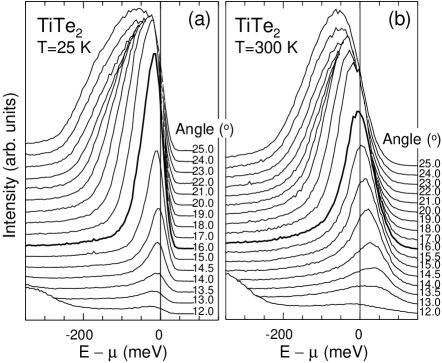
Figure 1: ARPES data of the Ti $3d$ band of TiTe₂ taken at $h\nu=21.2$ eV. Energy and angle resolutions are 35 meV and $\pm 1^{o}$, respectively. Thick lines are for $\mathbf{k}=\mathbf{k}_{F}$.

Fig. 1 shows our ARPES data taken at 25K and 300K. Previously, we have reported FL line shape fits of a 25 K data set [23, 24]. The new 25 K data in Fig. 1 are practically identical with our previously reported data [23, 24]. Note that the constant intensity at high binding energy, at least part of which is due to inelastic background, is negligibly low compared to the peak height in the data.

In previous reports [23, 24], we have shown that the line shapes at low $T$ are described well by Eq. 1 with a FL theory. The FL theory that we used in Ref. [References] is a simple phenomenological causal theory that has the correct FL behavior at low energies and satisfies the spectral sum rule on the global scale. As explained in Ref. [References] in detail, this theory involves two poles in the Green’s function, a quasi-particle pole and a “background” pole. The overall line shape evolution as a function of $|\epsilon(\mathbf{k})|$ shows crossover from a heavy quasi-particle band dispersion to an un-renormalized band dispersion. In the crossover region, the two poles interfere to produce an interesting two peak line shape, which we identified with the exceptionally broad line shape at large angles (e.g. 25^o). This crossover behavior is quite analogous to the similar behaviors found in the strong electron-phonon coupling systems [25, 26, 27] or in the HTSC’s [28]. The main finding of the previous fit efforts was that the quadratically falling tail at the high binding energy side of the peak distinguishes the FL model from other models. Here, we will focus on the temperature dependence of the line shape.

Eq. 1 shows that $T$ dependent line shape changes can occur due to both $A$ and $f$. For TiTe₂, which undergoes no phase transition or crossover, the change in $A$ is expected to be simply a gradual increase in the line width as $T$ increases. Without knowing the exact $T$ dependence of $A$, we will first ignore it as an approximation, and then investigate to what extent this approximation departs from observation. The $T$ dependence of the Fermi-Dirac function $f$ is simple: the step at $\mu$ becomes wider and flatter. The $T$-linear increase of the step width means that a larger portion of $A$ above $\mu$ becomes visible in photoemission.

Within this approximation, the most outstanding feature of the ARPES data at 300 K, i.e. that the dispersing peak is observed across $\mu$, can be understood by simple considerations. Near $\mu$, the intrinsic quasi-particle spectral function is approximately a delta function. However, the finite angular resolution requires that the spectral function must be summed over a momentum window $\Delta\mathbf{k}$ to give an effective energy width $\hbar v^{\prime}_{F}\Delta\mathbf{k}$ where $\hbar v^{\prime}_{F}$ is the peak velocity near $\mu$. Taking the FWHM of the $\omega$-derivative of $f$, the width of the step in f is approximately $4k_{B}T$. An interesting case occurs if this width is larger than the width of the peak, $\hbar v^{\prime}_{F}\Delta\mathbf{k}$. In this case, a peak slightly, say $k_{B}T$, above $\mu$, has most of its intensity above $\mu$, so that even after the multiplication by $f$ in Eq. 1, the line shape shows a peak above $\mu$. For the current case, $\hbar v^{\prime}_{F}$ is $\sim 0.5$ eVÅ and $\Delta\mathbf{k}$ is $0.07$ Å^-1, which gives an estimate of $\hbar v^{\prime}_{F}\Delta\mathbf{k}=35$ meV. At 300 K, $4k_{B}T=100\mathrm{meV}$, significantly larger than 35 meV, and indeed, we see the peak crossing $\mu$.

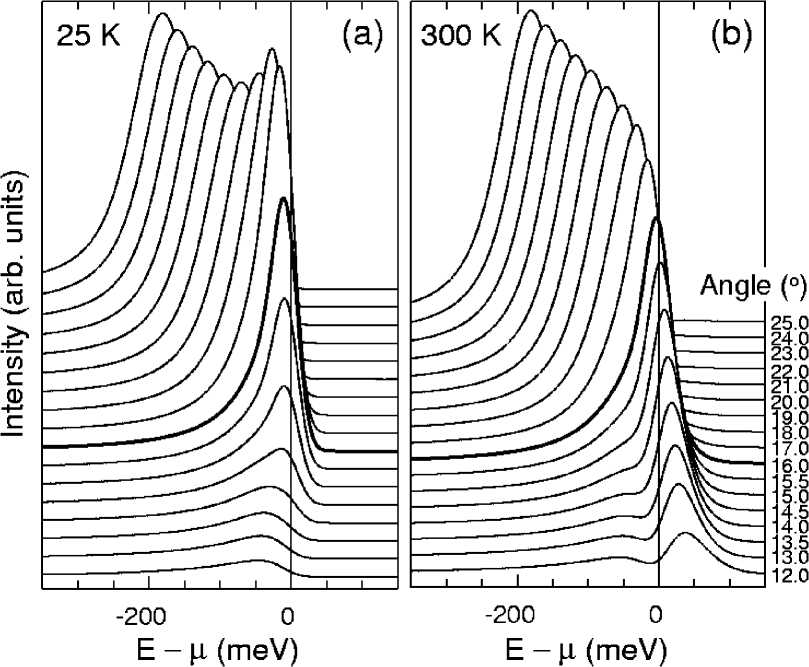
Figure 2: FL line shape simulations for the data of Fig. 1. The model parameters [24] are $Z/Q=0.4$, $Q\hbar v_{F}=0.6$ eVÅ, and $1/\beta^{\prime}=40$ meV. Thick lines are for $\mathbf{k}=\mathbf{k}_{F}$.

This argument is well supported by our line shape model calculation, shown in Fig. 2, using the Green’s function used in Ref. [References]. In this calculation, the $\mathbf{k}_{F}$ angle is defined to be 16^o. Other parameter values are in the vicinity of the values used in Ref. [References], and are chosen to describe the line shape near the 16^o spectrum shown in Fig. 1. For illustration purpose, the electron band dispersion is taken to be linear. The salient experimental features are reproduced well, i.e. the peaks and their back-bending below $\mu$ at 25K and their appearance across $\mu$ at 300K. Note that at 25K, $\mu$ lies very close to the top of the peak for $\mathbf{k}\approx\mathbf{k}_{F}$. This happens because the line shape near the FS crossing is a sharp peak very close to $\mu$, which is then pushed slightly to the left side of $\mu$ by the function $f$. This can occur whether the line shape is FL or non-FL, as long as there is a sharp peak near $\mu$. We note that ARPES peaks above $\mu$ have been previously demonstrated beautifully for Ni [29]. However, the three dimensional nature of Ni makes a line shape analysis much more difficult.

To be sure, there are differences between the data and the line shape calculations. First, the line shape calculated at 300K is too sharp – after crossing it shows a distinct two-peak structure which is not observed in the data. We attribute this to additional broadenings expected at high temperature but not included in the modeling – i.e. failure of our approximation of a $T$ independent $A$. As the result, the theoretical simulation shows peaks dispersing above $\mu$ farther up in energy, while in the experiment the peak reaches a maximum energy at 14^o and then bends back. Second, there are small differences in various estimates of k_F that one can make based on the line shapes. This is of great significance because $\mathbf{k}_{F}$ is one of the most basic quantities in condensed matter physics. Therefore we discuss this matter in the rest of this section.

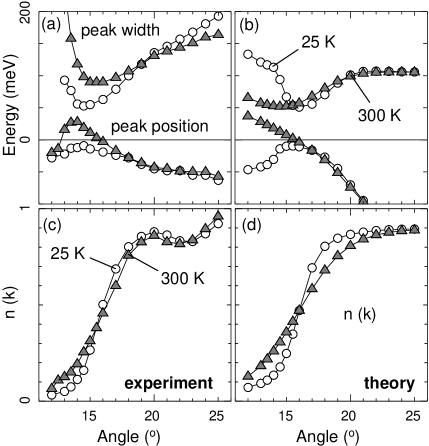
Figure 3: Line shape attributes of experimental (Fig. 1) and theoretical (Fig. 2) line shapes.

We summarize in Fig. 3 the peak position, peak width, and area under the spectrum as a function of k. The various k_F estimates are summarized in Table 1. In the theory, the various estimates are in quite good agreement with each other, if we ignore the 300 K peak width criterion which is expected to be rather unreliable due to the neglect of the $T$ dependent broadening in $A$, but in the data, they differ significantly. Notably, the minimum line width and the minimum binding energy criteria applied to the 25 K data give significantly lower values for k_F.

Criterion	theory	experiment
Peak position (300 K)	16o	16o
Peak width (300 K)	14.5o	15.0–16.0o
Peak position (25 K)	16.5o	14.5o
Peak width (25 K)	16o	14.5o
Fixed point of $n(\mathbf{k})$	16o	15.5o

Table 1: Various estimates of the $\mathbf{k}_{F}$ angle for line shapes of Fig. 1 and Fig. 2. The true $\mathbf{k}_{F}$ angle in the theory is 16^o, by definition.

The results in Table 1 are rather alarming. The two groups of criteria, one being the minimum binding energy and minimum line width at 25 K and the other being the rest, are all good criteria in theory. However, applied to the data, the two groups of criteria give quite different results. The question is then which criterion is the most robust. We argue that this is the peak-crossing criterion at 300K, because it relies on the single fact that effectively the total spectral function $A$ is observed in the $\mathbf{k},\omega$ region of interest, due to the slow variation of $f$ in Eq. 1. In contrast, the k_F value extracted from data using the first group of criteria, 14.5^o, is clearly not good because at this angle the ARPES peak exists above $\mu$ at 300K, a fact very hard to understand if this were indeed the crossing point.

In the least squares fit procedure applied to the 25 K data in Ref. [References], the k_F value was determined, not surprisingly, to be 14.5^o. Our conclusion is then that this is not a robust feature of the fit. We have demonstrated [30] that the fit can give the correct k_F value if other effects are included in the theory, such as electron hole asymmetry, k-mass, impurity scattering, and the uncertainty in the chemical potential. Recently, Kipp et al. [31] presented a temperature differential method to determine the k_F value for their TiTe₂ data, and determined the k_F angle to be 16.6^o. Their criterion is in principle equivalent to our $n(\mathbf{k})$ fixed point criterion, which, as Table 1 shows, gives a result similar to that from our best criterion. However, we note that the absolute value of their k_F angle differs from ours by $\sim 1^{o}$, which we interpret to mean that the data are different. In addition, we have some cautionary remarks about the $n(\mathbf{k})$ criterion. First, the argument of Ref. [References] depends critically on the assumption of the electron-hole symmetry (within the energy range of $\mu\pm 2k_{B}T$). Such symmetry may be more the exception than the rule. Second, any $T$ dependence in $A$ will move the fixed point of $n(\mathbf{k})$ away from k_F. In contrast, the observation of the peak crossing $\mu$ gives a more robust criterion for k_F. First, electron hole asymmetry gives an asymmetric line shape but no change in peak position. Second, $T$ dependence in $A$ broadens the line shape and gives a narrower range of momentum over which the dispersing peak across $\mu$ is observed, as we infer from the comparison shown in Fig. 3. However, as long as the dispersing peak is observed across $\mu$ for a finite range of $\mathbf{k}$, the determination of $\mathbf{k}_{F}$ is not affected.

It is an interesting question how our results can be generalized to other materials. The condition $4k_{B}T\gg\hbar v^{\prime}_{F}\Delta\mathbf{k}$ can be satisfied for either large $T$, small $v^{\prime}_{F}$ or small $\Delta\mathbf{k}$. Note that the current state of the art Scienta analyzer provides a $\Delta\mathbf{k}$ which is about a factor of 10 smaller than that used here, so that the condition $4k_{B}T\gg\hbar v^{\prime}_{F}\Delta\mathbf{k}$ can be easily satisfied for most materials at moderately high temperatures. Therefore, it should be examined whether a behavior similar to that reported here can be observed in other materials. If it turns out that such behavior is not observed despite the condition $4k_{B}T\gg\hbar v^{\prime}_{F}\Delta\mathbf{k}$, then that is a sign that the intrinsic line shape is too broad or that the assumption of a dispersing peak representing a metallic band is wrong.

5 Li_0.9Mo₆O₁₇ – non-CDW non-FL Line Shape

5.1 Background

Li_0.9Mo₆O₁₇ is a quasi-1D metal with two phase transitions, at 24 K and 1.9 K. The transition at 24 K ($T_{x}$) is not understood well, and that at 1.9 K is a superconducting transition. The lowest temperature of our PES measurement is 12 K, so hereafter we will concern ourselves with the phase transition at $T_{x}$ only. This transition shows up as a hump in the specific heat [32] and a resistivity uprise [33]. However, no gap opening is observed in the magnetic susceptibility [34] and the optical reflectivity [35]. Furthermore, no structural distortion is observed in X ray diffraction [36]. Therefore, we conclude that the transition is not a CDW transition, because these measurements routinely detect CDW gaps and Peierls lattice distortions in other materials such as the blue bronze. Nevertheless, one may be tempted to explain the resistivity uprise below $T_{x}$ as a gap opening. Then a gap (2$\Delta$) of 0.3 meV [33] would be estimated. Even if this gap picture is valid [37], such a gap is clearly not an ordinary CDW gap. Also, it should be noted that there exists an explanation [34] based on localization physics.

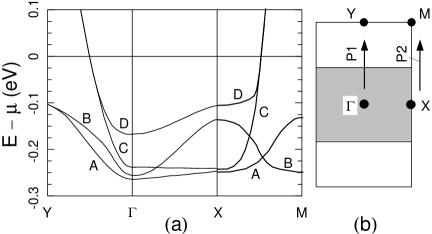
Figure 4: (a) Band dispersions and (b) FS of Li_0.9Mo₆O₁₇. These results are taken from the band theory of Ref. [References], except for the bands along the XM direction, which are sketches of the extension of the theory, based on our ARPES data.

The band structure of the Li purple bronze was calculated along the $\Gamma$X and $\Gamma$Y directions by Whangbo et al. [38], and is reproduced in Fig. 4. For completeness the figure also shows dispersions along XM deduced from ARPES data presented further below. According to the calculation, there are four orbitally non-degenerate Mo $4d$ bands near $\mu$. The four bands are labeled as A,B,C and D in the order of decreasing binding energy at the $\Gamma$ point. Only C and D cross $\mu$ and they become degenerate before the crossing. The calculated FS is perfectly 1D, and is given by $k_{\Gamma Y}=0.45\Gamma Y$. Note that each of the A,C and D bands show large and similar dispersions along the $\Gamma$Y direction and along the XM direction, while showing only minor dispersions along the $\Gamma$X direction. On the other hand, the band B shows similar dispersions along the directions $\Gamma$X and $\Gamma$Y, and shows opposite dispersions along the directions $\Gamma$X and XM, parallel to the 1D chain.

So far, three groups have reported ARPES data on the Li purple bronze. Initial data taken by Smith et al. [39] and our group [13] show almost dispersion-less peaks with $\mu$ crossings implied only by a spectral weight change. Subsequent data taken by Grioni et al. [40] with improved energy resolution, 15 meV, showed a hint of states crossing $\mu$, but these authors could not identify any crossing because their angle sampling was coarse and because the dispersing peak intensity was very weak. Our recent study [41] made use of a geometry in which the bands C and D are strongest along a special $\mathbf{k}$ path, P2 of Fig. 4, and discussed the observed non-FL line shape. We will summarize this result in the next section. Shortly after, Xue et al. [42] reported their new result obtained with a Scienta SES 200 analyzer, the observation of a Fermi edge in $\mathbf{k}$-summed ARPES spectra above $T_{x}$, implying FL line shapes, and also a gap opening below $T_{x}$. The gap below $T_{x}$ was cited as being consistent with the resistivity measurement, discussed above. Their finding of a FL line shape, in conflict with not only our data [41] but also all the preceding data, was then attributed to the high angular resolution of the new spectrometer. In our recent Comment [43] (also, see the Reply [44]), we pointed out that (i) the basic band structure implied by their data is in conflict with the band structure that emerges coherently from band theory, our data and that of Grioni et al. [40], (ii) our newly acquired similarly high resolution data show the band structure same as the latter and continue to show non-FL line shapes, (iii) their differing conclusion of a Fermi edge does not flow from higher angle resolution, but rather from the fundamental difference in the data, and (iv) their reported gap (80 meV) immensely exceeds the value 0.3 meV implied in a gap model of the resistivity. In this section, we give a more complete summary of our data than was possible in previous publications, and also recapitulate some essential findings of our published works. More details to support the points of our Comment can be found in Sections 5.2, 5.4 and 5.5, for points (iv), (i and ii) and (ii and iii) respectively.

5.2 Absence of PES Gap Opening

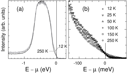
Figure 5: $T$ dependent angle integrated PES data for Li_0.9Mo₆O₁₇, measured at $h\nu=33$ eV, $\Delta E=30$ meV, $\Delta\theta=\pm 6^{o}$.

Perhaps the single most important feature of the Li purple bronze is that it is, up to now, unique as a non-CDW quasi-1D metal studied by ARPES. In this regard $T$ dependent PES is of great interest. Fig. 5 shows our result, which does not show any sign of a gap opening, within the energy resolution. The only observable change in the line shape is the sharpening of the leading edge scaling with temperature [45]. Our finding here is consistent with other measurements discussed above, and does not necessarily preclude the possibility that there is a small non-CDW gap. We expect that such a gap, if it exists, would have a value similar to or less than the value 0.3 meV implied in a gap model of the resistivity.

5.3 ARPES Line Shape – Comparison with LL

The Li purple bronze is a good candidate for being a LL at $T\gg T_{x}$, because its electronic structure is highly 1D [41] and is free of CDW formation. Gapping associated with the phase transition at $T_{x}$, if it occurs at all, is on such a low energy scale that a simple pseudo-gap effect cannot underlie the NFL properties observed above $T_{x}$.

LL Theory

A LL is defined as a system whose low energy fixed point is given by the Tomonaga-Luttinger (TL) model [46, 47]. In this model, electrons obey a linear band dispersion relation and the electron-electron interaction is truncated so that electrons undergo only forward scattering. An amazing feature of this model is that it is exactly solvable. The solution is characterized by two key features which distinguish a LL from a 3D FL system: (1) an anomalous dimension $\alpha$ and (2) spin-charge separation. The first directly implies the absence of Landau quasi-particles and the second means that the spin and charge quantum numbers of an electron are carried by distinct elementary excitations, i.e. waves of the spin density and the charge density.

PES line shapes for the TL model at $T=0$ are known in detail [48, 49]. The angle integrated spectrum vanishes as a power-law $|\omega|^{\alpha}$ at $E_{F}$. ARPES spectra for $\mathbf{k}$ inside the FS have two peaks (or one peak and an edge if $\alpha>0.5$) at positions corresponding to charge and spin wave energies at $\mathbf{k}$, and an edge for $\mathbf{k}$ outside the FS. We use the TL model [48] obtained by truncating the general electron-electron interaction of a continuum band to forward scattering only. In this TL model with repulsive spin-independent interactions, the spin velocity $v_{s}$ is equal to $v_{F}$, the charge velocity $v_{c}$ exceeds $v_{F}$ by a factor $\beta$ that is determined entirely by $\alpha$, and the edge singularity for $\mathbf{k}$ outside the FS disperses with velocity $v_{c}$. We note that $v_{s}=v_{F}$ is a property of a spin-rotationally invariant interaction in this TL model, but not in the most general form of the TL model [49]. For example, in the 1D Hubbard model which is spin-rotationally invariant and can be mapped onto the TL model in the low energy scale [50], $v_{s}$ is strongly renormalized. Similarly, the relation between $\alpha$ and $\beta$ of Ref. [References] is particular to the TL model used there. However, because the electronic states giving rise to the quasi-1D properties of the Li purple bronze are based on an extended Mo $4d$ wave-function, we believe that the TL model of Ref. [References] is the most appropriate starting point.

Solutions of the TL model can be extended to include weak interchain couplings [51] and finite temperature [52, 53]. These calculations show that the low energy LL behavior is modified within the energy scales of the interchain hopping parameter $t_{\perp}$ and temperature $T$, but the theory remains essentially the same as that of the $T=0$ purely 1D model for energies larger than these. Therefore, it is clear that in order to compare theory with experiment, one needs to be aware of these energy scales and additionally a purely experimental energy scale – the energy resolution $\Delta E$. With this in mind, we will use the $T=0$ solution of the TL model and include the $T$ dependence of the ARPES line shape only through the multiplication of the $f$ function in Eq. 1. Note that the band theory and our $\mu$ intensity map [41] indicate $t_{\perp}\approx 0$ for the Li purple bronze, i.e. the FS is nearly flat as predicted by band theory (Fig. 4).

Comparison

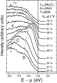
Figure 6: ARPES data of Li_0.9Mo₆O₁₇ along the path P2 at $h\nu=24$ eV, with $\Delta E=50$ meV and $\Delta\theta=\pm 1^{o}$.

We show our ARPES data [41] taken along the special path P2 in Fig. 6. So far, this data set remains as the one which shows the dispersing line shapes of both the $\mu$-crossing C,D excitations most strongly. This path was chosen to intersect a spot in our $\mu$ intensity map [41] that is exceptionally bright for the photon energy used and for the particular ARPES geometry of the Ames/Montana end-station.

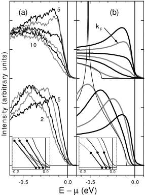
Figure 7: (a) A replot of the ARPES data of Li_0.9Mo₆O₁₇ in Fig. 6 and (b) LL theory simulation with $\alpha=0.9$.

Fig. 7 shows our comparison of the ARPES data of Fig. 6 with line shapes for a spin-independent repulsive TL model [48]. In the absence of any LL line shape theory including interactions between two bands, we apply line shapes calculated for the one-band TL model to the two degenerate bands crossing $\mu$. The value used for the anomalous dimension $\alpha$ was 0.9. The electron-electron potential screening length $r_{c}$ was taken to be 0.1 Å so that the calculated spectral functions are well within the validity limit of the universal LL behavior [54]. We chose the $v_{F}$ value so that for this value of $\alpha$ the renormalized charge velocity $\beta$$v_{F}$ ($\beta=5$ for $\alpha=0.9$) coincides with the linear dispersion that is observed over a range to $\approx 0.2$ eV below $\mu$ for peaks C and D while they are degenerate and to $\approx 0.5$ eV for peak C alone. Thin lines in Fig. 7 (b) show $A(\mathbf{k},\omega)$ without any experimental broadening, and demonstrate the charge peak and the spin edge for $\mathbf{k}$ inside the FS and the charge edge for $\mathbf{k}$ outside the FS. The theoretical simulation gives the $\mu$ weight close to that of the data, that being the reason for choosing an $\alpha$ value a little larger than the value 0.6 deduced from the power law exponent for the angle integrated spectrum [30]. Similarities of the theory and the data also include the velocity $v_{s}$ = $v_{F}$ of the leading spin edge movement before crossing (see insets), significant because the agreement is not forced by our procedure for choosing parameter values, and the loss of a spectral peaky upturn after the crossing. The general goodness of the agreement for spectra 5 through 7 leads us to take the value $k_{\Gamma Y}=51$% of $\Gamma Y$ as our best estimate for $\mathbf{k}_{F}$. Differences between the data and the theory include there being more intensity in the gap region before crossing and there being a much slower backward movement of the charge edge after crossing, which we attributed to the effects of 3D kinematics and to the presence of other bands not included in the model, respectively.

5.4 ARPES and Band Theory

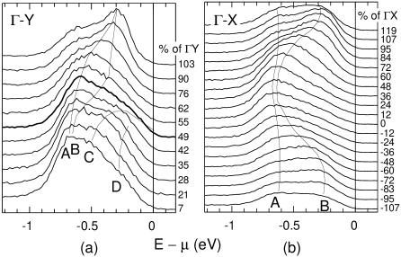
Figure 8: ARPES data of Li_0.9Mo₆O₁₇ taken along $\Gamma$Y ($T=200$ K) and $\Gamma$X ($T=50$ K), at $h\nu=24$ eV, $\Delta E=100$ meV, $\Delta\theta=\pm 1^{o}$. Thick line corresponds to $\mathbf{k}=\mathbf{k}_{F}$ spectrum.

It is equally as important to know the global band structure as it is to know what happens near the $\mu$ crossing. Fig. 8 shows ARPES data along $\Gamma$X and $\Gamma$Y. The sample surface is literally the same as the surface used in Fig. 6. Here, the most easily observed features are the A,B bands. Along $\Gamma$Y, band C is observed to cross $\mu$ and a hint of D is seen near the $\Gamma$ point. The data along $\Gamma$X show the A,B bands most clearly. Note also that there is an unexplained tendency, seen also [13] in other compositionally similar bronzes KMo₆O₁₇ and NaMo₆O₁₇, for non-dispersive weight to cling to the bottom of the band.

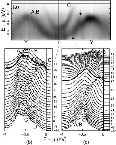
Figure 9: (a), (b) ARPES data of Li_0.9Mo₆O₁₇ taken along $\Gamma$Y at $h\nu=24$ eV, $T=250$ K, $\Delta E=35$ meV, $\Delta\theta=\pm 0.18^{o}$ and (c) at $h\nu=30$ eV, $T=200$ K, $\Delta E=36$ meV, $\Delta\theta=\pm 0.18^{o}$. For the meaning of arrows in (a), see text. Thick lines in (b) and (c) are $\mathbf{k}=\mathbf{k}_{F}$ spectra.

The data taken along $\Gamma$Y with the Scienta analyzer are shown in Fig. 9. The gray scale map, shown in (a), spans more than 1.5 unit cells in $\mathbf{k}$ space. This map was obtained by merging 12 overlapping angular mode Scienta data, and therefore the intensity profiles in the overlapping angle (i.e. momentum) regions do not always connect perfectly smoothly (e.g., see regions pointed by arrows) due to the discontinuous change of the ARPES geometry from one angular scan to the next. Nevertheless, it is clear that the map shows the C band dispersing to $\mu$, and that the dispersions of the A,B bands are consistent with the bulk crystal periodicity. EDC’s are shown in (b) and (c). Here, due to the better angle and energy resolutions, the bands are resolved better than in Fig. 8. In particular, the C band is clearly observed to cross $\mu$ in (b) and (c). In (b), the splitting of the A,B bands is clearly observed. The small difference between the $\mathbf{k}_{F}$ value for these data and that for the preceding ARPES data is attributed to a small variation of the Li ion numbers on the surface for different cleaved surfaces. Note also that the line shape at $\mathbf{k}_{F}$ shows an increased $\mu$ weight relative to the peak height. We attribute this to the improved angle resolution, which we will discuss shortly.

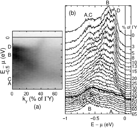
Figure 10: Scienta data of Li_0.9Mo₆O₁₇ taken along the special direction P2 (Fig. 4) at $h\nu=24$ eV, $T=30$ K, $\Delta E=26$ meV and $\Delta\theta=\pm 0.18^{o}$. Thick line corresponds to $\mathbf{k}=\mathbf{k}_{F}$ spectrum.

The experimental bands observed along $\Gamma$Y and $\Gamma$X are in good agreement with the band theory of Fig. 4, except for the overall band width. We now show Scienta data taken along the special path P2 in Fig. 10. Compared to the data of Fig. 6, the peaks are clearly better resolved. Especially, the bands B and D are completely resolved, much like in the band theory. As a result, the dispersion of peak B, which could not be observed in the data of Fig. 6, is now clearly observed, and the dispersion of peak D is now clearer. Note that the relative intensities of the peaks in this data set are not identical with those of Fig. 6. The difference is due to the difference in the geometry of the two experiments, i.e. a different photon incidence angle relative to the surface normal. In particular, the peaks C,D are not as strong as in Fig. 6. Even so, the line shape at the $\mu$ crossing point is clearly observed and shows much more weight than that of the line shape of Fig. 6. We discuss this aspect of the data next.

5.5 Discussion

In the last section, we showed that the $(\mathbf{k}_{F},\mu)$ weight increases as the angle resolution is improved. This is an expected general behavior if the $\mathbf{k}=\mathbf{k}_{F}$ spectrum is strongly peaky at $\mu$. For example, the TL line shape for $\mathbf{k}_{F}$ has a power law behavior $|\omega|^{\alpha-1}$, diverging at $\mu$ for $\alpha<1$. Therefore, as is easily shown by direct numerical simulation, when the angle resolution is improved gradually, the $\mu$ weight steadily increases. Thus the mere observation of more $\mu$ weight with better angle resolution is not by itself evidence for a FL line shape. In fact, with regard to the weight at $\mu$, the only sure way of distinguishing the FL and non-FL line shapes is to examine the angle integrated spectrum.

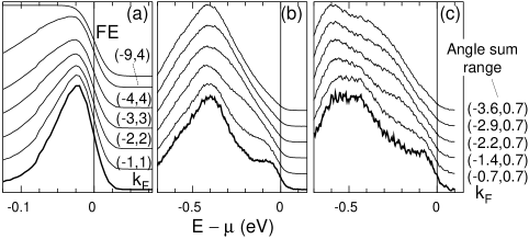
Figure 11: Progressive angle integration of (a) TiTe₂ data (Fig. 1 (a)), (b) Li_0.9Mo₆O₁₇ data (Fig. 9 (c)), and (c) Li_0.9Mo₆O₁₇ data (Fig. 9 (b)). The negative (positive) number in the angle sum range means the angle for which the band energy $\epsilon(\mathbf{k})$ is negative (positive). In (a), a Fermi edge (FE) is drawn at the top. (b) and (c) have the same formats. The stated angle sum range does not include the inherent angle resolution of an individual spectrum, $\pm 1^{o}$ for (a) and $\pm 0.18^{o}$ for (b) and (c).

Theoretically the $\mathbf{k}$-sum (angle integration) of the FL line shape and that of the TL line shape give quite different results. The former gives a Fermi edge and the latter gives a power law. It is very important to test whether this difference can be seen experimentally. Here we examine the data from our FL reference TiTe₂ and from the Li purple bronze to see if this theoretical scenario comes true. Fig. 11 shows the result. As more and more angles are summed, the TiTe₂ line shape converges to a Fermi edge shape. The steep decrease on the high binding energy side of the spectrum is due to the narrow band width of the Ti $3d$ band. In great contrast, the line shape for the Li bronze loses the edge shape rapidly as more and more angles are summed, converging to the power law behavior we have observed using an angle integrating spectrometer in our home lab [30]. Our observation here directly contradicts the claim of Xue et al. [42] of a Fermi edge in a partially angle integrated spectrum.

The Li purple bronze remains as a unique case of a CDW-free quasi-1D metal accessible by photoemission. The global band structure is well understood in both theory and experiment. Furthermore, the two main characteristics of the LL, the anomalous dimension $\alpha$ and the spin-charge separation, are identified in the data, the former in the absence of Fermi edge and the power-law onset of the angle integrated spectral function and the latter by interpreting, appropriately for $\alpha>0.5$, the $\mu$-crossing peak as the charge peak and the extrapolated finite energy onset of the peak as the spin edge. Among these features the spin edge is perhaps the least convincing feature due to the smoothness of the edge in the data. A likely source of this smoothness is 3D kinematics, as we mentioned at the end of Section 5.3. Also, the spin velocity itself needs to be understood better. Within the TL theory used here, it is supposed to be the same as the band velocity, but the value used in our line shape analysis is about a factor of 2 too small compared with the value of the band theory (Fig. 4). This may be due to the inaccuracy of the tight binding calculation or the simplistic nature of the LL theory we used. For example, it is reasonable to think that the backward scattering terms, completely neglected here, will in reality have a residual effect of changing the relation between $\alpha$ and the spin and/or charge velocity, analogously to the Hubbard model case mentioned in Section 5.3. Therefore, a more detailed understanding calls for a first principles band theory and a better understanding of the electron-electron interactions.

6 Blue Bronze – CDW non-FL Line Shape

6.1 CDW Theory

Because the CDW is an essential ingredient for describing the physics of the blue bronze, we start this section with a discussion of CDW theory. The so-called FS nesting condition, that one part of the FS matches another part of the FS via a translation by a single wavevector, implies an instability towards the formation of a CDW with periodicity given by the nesting vector and the consequent formation of a CDW gap at $\mu$ [6]. Via electron-phonon coupling, the lattice is distorted with the same wave vector. The nesting condition is fulfilled perfectly in 1D, and can be met approximately but with increasing difficulty in 2D and 3D. In the standard mean-field description of the Frölich Hamiltonian [55], which is formally equivalent to the BCS theory of superconductivity, a phase transition occurs at a finite temperature $T_{c}$ where the lattice modulation at the nesting vector becomes static. Below $T_{c}$, the CDW gap opens up with the same $T$ dependence as the BCS gap. Above $T_{c}$, the electronic state is that of a simple FL metal.

The mean-field picture of the CDW requires significant modification to account for fluctuations, especially in low dimensions. In fact, for a perfectly 1D system, a finite $T$ phase transition does not occur, due to the well known fact [56, 57] that in 1D the entropy increase associated with the break-up of long range order into many short range orders wins over the energy minimization associated with the long range order. Therefore, it is obvious that a CDW fluctuation theory must be also a 3D theory in order to have the power to predict a realistic finite $T$ phase transition.

Much work has been done on CDW fluctuations. A study by McKenzie and Wilkins [58] predicts a significant filling-in of the gap region at low $T$ due to CDW fluctuations and also quantum lattice fluctuations. Most theories are concerned however with $T\geq T_{c}$. Some theories [59, 60] treat fluctuations exactly but deal with a single 1D chain, and others, e.g. that of Rice and Strässler (RS) [61], treat fluctuations perturbatively but include interchain couplings. We find the latter type of theory to be more useful because there are enough ingredients to permit a realistic comparison to experiments. We also find that the line shapes predicted using the former type of theory, specifically that of Sadovskii [59], are actually quite similar to those predicted by the RS theory for the same correlation length.

The result of the RS theory is summarized in its self energy, $\Sigma_{RS}(\mathbf{k},\omega)$,

$$\frac{\psi}{-i\,f}\,\log\left(1-\frac{i\,f}{\omega/\psi-\epsilon(\mathbf{k}\pm\mathbf{q}_{CDW})/\psi-i\,\gamma}\right)$$ (2)

where $\psi$, $f$ and $\gamma$ are all $T$ dependent quantities. $\psi$ is the “pseudo-gap” parameter, i.e. the root-mean-square fluctuation of the order parameter, and $\gamma=\hbar v_{F}/(\xi\psi)$ where $\xi$ is the correlation length of the CDW fluctuation. The parameter $f$ is basically an effective 3D coupling strength parameter, and distinguishes this theory from that of Lee, Rice and Anderson (LRA) [62], which is a perturbative 1D theory. RS theory predicts, in the limit of strong fluctuation (i.e. $f\leq O(1)$),

$$T_{c}/T_{MF}=0.26f(T_{c})^{1/3},$$ (3)

which implies $T_{c}\ll T_{MF}$.

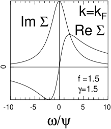
Figure 12: Self energy for the RS theory. Theoretical parameters are those for our simulation of blue bronze data at 250 K.

The self energy of Eq. 2 is shown in Fig. 12. In contrast to the situation in the simple mean-field solution, the normal state is not a FL in this theory. Im$\Sigma$ has a finite value and a negative curvature at $\mu$, and Re$\Sigma$ has a positive slope at $\mu$, directly contradicting the well-known FL self energy behavior [63]. These properties were pointed out by McKenzie [64] for Sodovskii’s results.

6.2 Background

K_0.3MoO₃, is one of the most intensely studied CDW materials, and yet some basic properties are still difficult to understand. Its CDW wavevector, studied by X ray diffraction [65] and neutron scattering [66], is unusual in that it shows a $T$ dependence. The magnetic susceptibility and the resistivity measurements are intriguing because in the normal state, the magnetic susceptibility increases steadily up to the highest measured temperature of 720K [67] while the resistivity shows perfectly metallic behavior. Later in this section we will discuss these issues further.

The crystal structure of the blue bronze is centered monoclinic [68, 69], and the repeating motif is the Mo₁₀O₃₂ chain which defines the $b$ axis – the “easy” axis. The quasi-1D nature of the electron conduction is shown by the resistivity [70] and the optical properties [71]. The basic band structure was calculated first by Whangbo and Schneemeyer [72]. The calculation shows that two orbitally non-degenerate Mo $4d$ bands are partially occupied by electrons donated by the K⁺ ions, making the material conducting. In the notation of these authors, which we follow here, the BZ boundary along the quasi-1D b axis is called the X point, and we wish to remind readers that the equivalent point for the Li purple bronze was called the Y point in Section 5.

Veuillen et al. [73] first reported ARPES results on the blue bronze. Their result shows a single broad peak dispersing to a $\mu$ crossing at a k value in good agreement with the CDW wavevector. A subsequent high resolution angle integrated PES study by Dardel et al. [74] showed a spectrum with anomalously low $\mu$ weight and no distinct Fermi edge. They also reported $T$ dependent data [75] which showed evidence of a CDW gap opening. Breuer et al. [76] did a detailed study of the surface damage caused by photon and electron/ion bombardment. The major symptom of surface damage is the emergence of a peak at $\sim 2$ eV binding energy and the shift of the spectral weight at $\mu$ to higher binding energy. By taking precautions to minimize photon bombardment above the absorption threshold energy ($>36$ eV), we have obtained ARPES spectra [13, 77] with strikingly low inelastic background and two dispersing peaks crossing $\mu$. We have also demonstrated [13] that the two dispersing peaks cross $\mu$ at different k values by taking a $\mu$ intensity map. The two dispersing peaks were subsequently reproduced by Grioni et al. [40], and more recently by Fedorov et al. [78]. The latter authors also reported a $T$ dependence of the nesting vector measured in ARPES along $\Gamma$X to be in good agreement with that of the CDW wave vector measured in neutron scattering (See, however, our discussion in Section 6.5).

The non-FL line shape of the blue bronze, namely the absence of a PES Fermi edge, remains unexplained. In this section, we show that this feature is not reconcilable with the standard CDW picture even when the pseudo-gap mechanism is included.

6.3 Data

In this section we introduce some new ARPES data, as well as summarize some key results from the literature. In particular new $T$ dependent high resolution data are, to our knowledge, the first to show how the ARPES line shapes of the EDC’s change across $T_{C}$ (180 K).

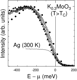
Figure 13: Angle integrated photoemission data of K_0.3MoO₃ in the normal metallic state. Filled circles: angle sum of data in Ref. [References] (also shown in Fig. 15), $h\nu=20$ eV, $\Delta E=100$ meV, $\Delta\theta=\pm 10^{o}$, $T=220$ K. Empty circles: this work, $h\nu=13$ eV, $\Delta E=27$ meV, $\Delta\theta=\pm 6^{o}$, $T=250$ K. Empty triangles and line: Ref. [References], $h\nu=21.2$ eV, $\Delta E=33$ meV, $\Delta\theta=\pm 12^{o}$, $T=300$ K. Filled triangles: Ref. [References], $h\nu=21.2$ eV, $\Delta E=20$ meV, $\Delta\theta=\pm 3^{o}$, $T=313$ K.

Fig. 13 shows various high resolution angle integrated photoemission spectra and contrasts them with a reference spectrum taken on Ag. These angle integrated spectra are taken in the metallic state well above the phase transition. Nevertheless, the Fermi edge that is characteristic of a 3D metal is completely absent. It is interesting to note that a related material, NaMo₆O₁₇, whose electronic structure is that of three weakly interacting 1D chains oriented at 120 degrees to one another in planes, does show a Fermi edge, as we reported in Ref. [References].

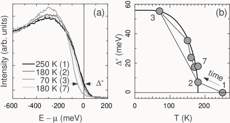
Figure 14: (a) $T$ dependent angle integrated photoemission data of K_0.3MoO₃. $h\nu=13$ eV, $\Delta E=27$ meV, $\Delta\theta=\pm 6^{o}$. (b) The “gap” parameter $\Delta^{*}$ deduced from data. The thick curve is the BCS gap function.

One may wonder whether the absence of the Fermi edge is merely the result of a bad surface, not representative of the bulk. However, this is not so. Our $\mu$ intensity map showed a FS consisting of two pairs of lines which imply a nesting vector in agreement with the CDW wavevector [66]. Also the bulk phase transition is clearly detectable in $T$ dependent measurement of angle integrated spectra [75]. Fig. 14 shows our own $T$ dependent PES data, taken with a Scienta SES 200 analyzer using its angle integrated mode. The sequence of $T$ in the measurement was 250 K, 180 K, 70 K, 150 K, 160 K, 170 K and 180 K. This $T$ sequence was deliberately chosen to reveal any effects of irreversible sample damage during the $T$ variation. The two 180 K spectra in Fig. 14(a), taken initially and at the end of the cycle, are almost identical with each other, indicating that the data are largely free from such an undesirable irreversibility.

The spectral change observed in Fig. 14 is in good agreement with the results reported in Ref. [References]. Below the transition point (180 K), the spectral edge moves to a higher binding energy, signaling gap opening. These spectra should be contrasted with those of Fig. 5 for the Li purple bronze, where a gap does not open. To exactly quantify the gap opening is a difficult task due to the odd line shape, and we define a first approximation $\Delta^{*}$ (see Fig. 14 (a)) as the shift of the spectral edge at the intensity value corresponding to $\mu$ at 250 K. Our method is different from the one used by Dardel et al. [75], i.e. taking the inflection point to quantify the gap opening, but gives similar results, shown in Fig. 14 (b). The difference at 180 K of the final point 7 from the initial point 2 is probably due to a slight degradation of the surface. Similar to the findings by Dardel et al. [75], the temperature variation of the gap opening is roughly BCS like. The $\Delta^{*}(T=0)$ value deduced from our procedure, 56 meV, is a lower bound, for reasons that we will discuss later.

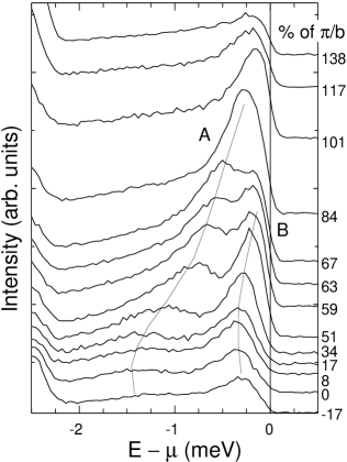
Figure 15: ARPES data of K_0.3MoO₃ taken at $h\nu=20$ eV, $\Delta E=100$ meV, $\Delta\theta=\pm 1^{o}$ and $T=220$ K. Thin lines are guides to the eye for dispersions.

Fig. 15 shows our early modest resolution high temperature ARPES data, most of which were already reported in Ref. [References]. This ARPES data set attests to a very clean surface because the background intensity level is very low and there is no sign of the defect peak at $2$ eV binding energy. For this reason, we have included the angle sum of this data set in the collection of angle integrated data of Fig. 13.

As we have shown before [13], the two peaks of Fig. 15 cross at distinct k_F values. The $\mu$ intensity map taken at $h\nu=17$ eV [13] shows that band B crosses at $\approx$62 % of $\pi$/b. The exact crossing point of band A is not easily determined because the map shows maximum intensity centered at the X point. Similarly the EDC’s of Fig. 15 and Ref. [References] show an almost symmetric band having a maximum at the point X. Therefore, in these moderate resolution data, we take the spectrum at the X point (e.g. the 101 % spectrum in Fig. 15) to be representative of the k $=$ k_F spectrum.

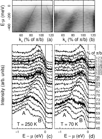
Figure 16: $T$ dependent ARPES data of K_0.3MoO₃ taken at $h\nu=13$ eV, $\Delta E=27$ meV, and $\Delta\theta=\pm 0.18^{o}$. Thin lines in (a) are guides to the eye for dispersions. Thick lines in (c) and (d) are $\mathbf{k}=\mathbf{k}_{F}$ spectra.

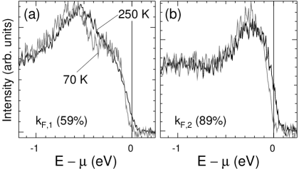
Figure 17: $T$ dependence of spectra at FS crossings for the K_0.3MoO₃ data of Fig. 16.

Fig. 16 shows our new high resolution data taken with $13$ eV photons near the X point at 250 K and 70 K. Each data set was taken immediately after taking the angle integrated 250 K and the 70 K spectra of Fig. 14, respectively, i.e., they were taken on an undamaged surface showing the CDW gap opening. This new data set is an improvement over the previous lower resolution data set, in that the crossing near the X point is now resolved due to better angle resolution. The $\mu$ intensity pattern shows a minimum at the X point, instead of a maximum, and it enables identification of FS crossing points for band A (90 %) and for band B (59 %). For later discussion in Sections 6.4 and 7, we directly compare the T dependence of the spectra at these crossing points in Fig. 17. From these crossings, we get an estimate of the CDW wavevector of 75 % of $b^{*}$, which seems to be in good agreement with the observed value which varies from 72 % to 75 % as $T$ varies from 180 K to 0 K. We note that from our $\mu$ intensity map [13] one cannot rule out a somewhat 2D FS for band A. In this case we would have an imperfect nesting condition such as we have observed for SmTe₃ [79] where the nesting vector along one particular direction (e.g. the $\Gamma$X direction) generally differs from that of the CDW wavevector, which is a compromise value determined by global energy minimization across the entire 2D FS.

A surprising finding from comparing the data of Fig. 15 and Fig. 16 is that the widths of the A,B peaks and also the $({\mathbf{k}}_{F},\mu)$ weight relative to the peak height do not change significantly as the angle resolution is improved. This is a direct spectroscopic contrast between the Li purple bronze and the blue bronze.

6.4 Line Shapes

In this section, we compare CDW and LL line shape theories with our data. The theories used here are single band theories, while there are actually two $\mu$ crossing bands in the blue bronze. The $\mu$ crossing line shapes of band B are obscured by the presence of band A, while those of band A are isolated near the X point. Therefore, our ARPES comparison is focused on band A.

CDW

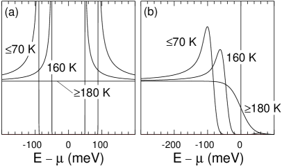
Figure 18: (a) Temperature dependent density of states and (b) angle integrated photoemission data calculated within the mean-field CDW theory. Strictly speaking, theory is $T$ dependent below 70 K, but is negligibly so. Experimental energy resolution for the data of Fig. 14 is included in (b).

An obvious starting point for comparing the data to theory is the mean field CDW theory. The prediction of the mean field theory for the ARPES line shape is simple: the band dispersion relation $\epsilon(\mathbf{k})$ is replaced by $-\sqrt{\epsilon(\mathbf{k})^{2}+\Delta^{2}}$ [80] and the gap $\Delta(T)$ has the BCS $T$ dependence. The magnitude of $\Delta(0)$ for the blue bronze shows a significant variation in the literature: $\sim 40$ meV (resistivity [81]), $\sim 50$ meV (magnetic susceptibility [67]) and $\sim 90$ meV (optics [82]). Hereafter, we will use the result from the optical measurement, consistent with taking our estimate of 56 meV to be a lower bound for $\Delta(0)$, as explained below. The angle integrated spectral functions calculated in the mean field theory are shown in Fig. 18.

The mean field CDW theory cannot adequately describe our photoemission data. First of all, the normal state angle integrated PES data do not show a Fermi edge (Fig. 13), in contrast to the calculation of Fig. 18. Second, the experimental line shape changes in the angle integrated PES data due to the CDW gap opening (Fig. 14) are difficult to understand. These changes include the low $T$ intensity pile-up occurring at a much larger energy $\sim 0.3$ eV compared to the gap energy, as was noted already by Dardel et al. [75], and the existence of the significant sub-gap tail at 70 K. Third, the peak shift by $-\Delta$ expected to occur for the $\mathbf{k}=\mathbf{k}_{F}$ ARPES data is not observable in Fig. 17. Instead, only an intensity redistribution within the ARPES peak seems to occur. This can be contrasted to the case of the high temperature CDW material SmTe₃ [79], for which the dispersion relation $-\sqrt{\epsilon(\mathbf{k})^{2}+\Delta^{2}}$ [80] is clearly observed.

It is an obvious next step to test whether the inclusion of CDW fluctuations improves the comparison of the data with the CDW theory. Evidences for CDW fluctuations are ample. Below $T_{c}$, a strong sub-gap tail is observed in optics [82], in qualitative agreement with the theory by McKenzie and Wilkins [58] and also with our observation of a strong sub-gap tail existing at 70 K. This is why we take our estimate $\Delta^{*}$ to be a lower bound. In this article, our main interest however is in the fluctuations in the normal state above $T_{c}$. Evidences for fluctuations above $T_{c}$ are the diffuse scattering observed by X ray experiments [83, 84], and the large value of $2\Delta(0)/(k_{B}T_{c})$, 5–12, compared to the mean field value 3.52.

Next we estimate parameters for the RS theory. For the estimate of $T_{MF}$, we use the mean-field relation $3.52k_{B}T_{MF}=2\Delta(0)$, and get $T_{MF}=590$ K for $\Delta(0)=90$ meV. Then, from Eq. 3, we get $f(T_{c})=1.5$. Then, the weak, and unimportant, $T$ dependence of $f$ is included as outlined in Ref. [References]. For our $f(T_{c})$ value, Eq. 9 of Ref. [References] gives $\psi(T_{c})=54$ meV. The pseudo-gap is expected to decrease as $T$ increases, and a calculation [85] does show such behavior. In our modeling, we simply ignore this $T$ dependence. By so doing, we are somewhat overestimating the pseudo-gap above $T_{c}$. Note that our estimate that $\psi(T_{c})$ is roughly half of $\Delta(0)$ is in good agreement with estimates by others [67, 81]. For $\hbar v_{F}$, we measure the peak dispersion in the ARPES data and get $\sim 4.5$ eVÅ for band A and $\sim 3$ eVÅ for band B. The nesting occurs between these two bands, and therefore $v_{F}$ to be used in the expression for $\gamma$ should be an “average” of these two values. Instead, we simply use the value for band B and again slightly overestimate the effect of the pseudo-gap. Lastly, for the correlation length $\xi(T)$, we use the result measured by X-ray diffraction [83, 86].

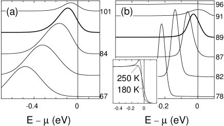
Figure 19: Simulation of CDW fluctuation line shape (a) for the data of Fig. 15 and (b) for those of Fig. 16 ($T=250$ K). Thick lines are $\mathbf{k}=\mathbf{k}_{F}$ spectra. Inset: Simulation of the data of Fig. 14 at 250 K and 180 K.

Fig. 19 shows our simulation. For the angle integrated spectrum shown in the inset, note that the simulation does show suppression of weight at $\mu$. However, the $\mu$ weight at 250 K is significantly larger ($35$ %) than that for the 250 K data of Fig. 14 (a) (25 %). Furthermore, the $T$ dependence observed above $T_{c}$ is far too weak compared to the simulation. Perhaps most importantly, the simulation shows a Fermi-edge-like line shape at 250 K, albeit with reduced $\mu$ weight, but this is not observed in the data.

The ARPES simulations shown in (a) and (b) of Fig. 19 give a more detailed view. Line shapes at and above $\mathbf{k}_{F}$ are most interesting. For both (a) and (b), the maximum $\mu$ weight occurs for $\mathbf{k}$ somewhat greater than $\mathbf{k}_{F}$. For the moderate resolutions used in (a), the $\mu$ weight at 101 % is significantly larger than half the peak height, but the data show slightly less than half. The comparison becomes more problematic for high resolutions used in (b). In this case, the peak occurs at $\mu$ for 91 %, and disappears quickly after that. Experimentally, however, the $\mu$ weight is never greater than half the peak height and the line shape after crossing is nearly the same as that at the crossing. In addition, notice that the large line width reduction from (a) to (b) is not observed in the data.

LL

In this section, we compare the blue bronze data with line shapes for a spin-independent TL model [48], in the same fashion as was done in Section 5. First, we examine whether the experimental data show the power law predicted by the LL theory. This can be done by examining the data of Fig. 13 in a log-log plot, and identifying the region where the plot is linear. As we noted before, this region is expected to start at a finite binding energy, determined by $t_{\perp}$, $T$ and $\Delta E$. We estimate an upper bound of $t_{\perp}$ to be $\approx 30$ meV [87]. The data of Fig. 13 show power law behavior, $\alpha=0.5-0.8$, starting from energy $\approx\max(2k_{B}T,\Delta E/2,t_{\perp})$ to 150–200 meV. The variation of the $\alpha$ value seems to correlate with $T$, but may also have correlations with other factors such as angular resolution and sample. We choose the value of $\alpha=0.7$ obtained from our data taken at 300 K – the farthest from the phase transition – and having the largest angle acceptance.

Next we compare the ARPES data with the calculated TL model line shapes of Fig. 20. The parameters used for this TL model are $\alpha=0.7$, $\hbar v_{F}=0.98$ eVÅ, and $r_{c}=0.1$Å. The $v_{F}$ value was chosen in order to reproduce the dispersing peak with velocity 4.5 eVÅ. The $r_{c}$ value was chosen so that the calculated spectral functions are well within the validity limit of the universal LL behavior [54].

The theoretical angle integrated spectrum in Fig. 20 improves comparison with the data relative to that for the RS theory, in that the TL theory predicts less $\mu$ weight and no Fermi edge. The amount of $\mu$ weight has some uncertainty due to the fact that the theory here does not include $T$ and $t_{\perp}$. In its current form, the theory predicts less $\mu$ weight in the angle integrated spectrum than occurs in the data. Perhaps inclusion of $T$ and $t_{\perp}$ would make the agreement better in this regard.

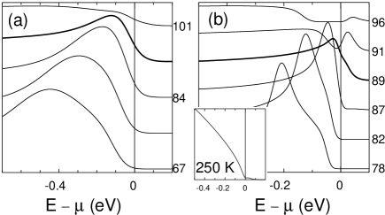
Figure 20: Simulation of LL line shape, in a similar fashion as Fig. 19.

The comparison to the ARPES data is more involved. While the generally lower $\mu$ weight than in the CDW RS theory is in better agreement with data, it is difficult to identify some key features of the $\mathbf{k}$-resolved theory in the data. The spin edge singularities, which provided an interpretation of the leading edges in the Li purple bronze line shapes, are hard to identify in the blue bronze data. The charge edge singularity after $\mu$ crossing is also hard to see. The high resolution simulation of (b) reveals discrepancies: the theory shows a peak above $\mu$ after crossing and a greatly reduced line width before crossing, none of which is observed in the data.

6.5 Discussion

The comparisons of the preceding section show that neither of the two theories explains the ARPES line shapes satisfactorily. The essential findings are that (1) the absence of a Fermi edge (up to 313 K; see Fig. 13) is very hard to reconcile with the CDW theory, (2) the higher resolution ARPES simulation for both theories predict too much weight at $\mu$ and too strong a $\mathbf{k}$ dependence for $\mathbf{k}\geq\mathbf{k}_{F}$, and (3) the edge line shapes in the LL theory are not identified in the data. The single EDC shown by Fedorov et al. [78] enable us to infer point (2) also from their data.

The severe disagreement of the high resolution data with theory needs careful thinking. Let us recall from Section 4 that if intrinsic line shapes are sharp enough, then it is possible to observe peaks moving above $\mu$, as is indeed the case for our TL line shape simulation of Fig. 20. That this behavior is not observed in the data then implies that the intrinsic line shape is not sharp enough. We have already noted in fact that the data do not show significant line width reduction upon resolution improvement. This implies that the ARPES line width is not resolution limited and is very large – a few hundred meV’s. The origin of such a large line width is an open question. A mundane explanation invoking a non-ideal surface condition – a mixture of mosaics or a warped surface – seems unlikely, because we observe two $\mu$ crossings at the X point (Section 6.3) and a sharp Laue diffraction pattern.

Underlying the reasoning in the preceding paragraph is the assumption that the intrinsic line shape is not gapped. However, this assumption is dubious for the blue bronze. As noted first by Voit [88], the normal state transport data shows spin-charge separation in that the spin susceptibility shows gapped behavior ($\Delta=20$ meV) while the resistivity shows metallic behavior. Therefore, he suggested that the Luther-Emery (LE) model [89] gives a good description of the normal state of the blue bronze. In this model, certain backward scattering between electrons is included, in addition to the forward scattering already included in the TL model, and a gap opens up in the spin channel. Because a single particle excitation involves simultaneous excitations of spin and charge, this spin gap appears in the single particle line shapes [53, 90]. Such a gap could be a reason why the $\mu$ weight does not increase further upon resolution improvement.

The contrasting behaviors of the spin susceptibility and the resistivity was recognized earlier by Pouget [91], who proposed a simple explanation within the one electron band theory. An essential component of this explanation is a flat band $56$ meV above $\mu$, which is thermally occupied as $T$ increases. This flat band also was used in an explanation of the $T$ dependent CDW wavevector. Indeed, the band calculation by Whangbo and Schneemeyer showed such a band near the $\Gamma$ point. If this scenario is right, then this shallow band should be detectable in ARPES at high $T$, e.g. in the normal state. However, this band is neither reproduced by new local density approximation (LDA) band calculations [92, 93] nor observed by ARPES. Therefore, the more exotic explanation for the $T$ dependent susceptibility by Voit, discussed in the previous paragraph, gains more credibility. The $T$ dependent CDW wavevector would then require an alternate explanation as well. Recently, Fedorov et al. [78] proposed a model in which $T$ dependent electron hopping integrals are responsible for the $T$ dependent CDW wavevector. However, the data presented by these authors are insufficient to support the model because the data were taken along a single line in the 2D BZ. In the model of the paper the 2D character of the FS is essential, implying imperfect nesting. Then the CDW wave vector should not be the same as the nesting vector along a single line. Very qualitatively, the 2D character of the FS found in our $\mu$ intensity map [13] appears to be less than envisioned in the model or predicted by band theory. In our opinion additional experiments and a further consideration of various models of the $T$ dependent CDW wavevector are merited.

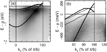
Figure 21: Comparison of ARPES and band calculations for the blue bronze. Thin lines are tight-binding calculation [72] and thick lines are LDA calculation [92].

One of the characteristics of the repulsive TL model is that the charge velocity is renormalized to be bigger than $v_{F}$, in contrast to the quasi-particle Fermi velocity smaller than $v_{F}$ in the case of the FL. It is therefore an interesting question how the ARPES dispersions compare with the theory. Fig. 21 shows the comparison. We show two band calculation results – the tight binding theory by Whangbo and Schneemeyer [72] and first-principles LDA theory by Kim et al. [92]. As noted previously [13, 77], the dispersion of band A is a factor of 5 larger, compared to tight binding theory, and that of band B is a factor of 2 larger. The new LDA theory, which should be more accurate, is quite different from the tight binding theory. The new LDA band calculation is confirmed by that of another group [93]. Therefore the uncertainties in the magnitudes of the one electron band dispersions seem finally to be gone. The dispersion of band A is in good agreement with that of the LDA theory and that of band B is still about a factor of 2 larger. This finding remains as a piece of the whole blue bronze puzzle, and seems to require a better understanding of the dependence of spin and charge velocities on $\alpha$ as we discussed in Section 5.5.

7 Concluding Remarks

In this article, we have discussed three examples of ARPES line shape studies of quasi-2D and quasi-1D samples showing FL and non-FL line shapes. The complex and intriguing line shapes of these prototypical materials are not completely understood, and we strongly feel that they are worth studying more both experimentally and theoretically, because they connect to fundamental concepts of condensed matter physics.

Before concluding we comment on the common aspects of the LL parameters for the bronzes, the large $\alpha$ and energy scale. In the TL model description we used an $\alpha$ value of 0.7 (blue bronze) and 0.9 (Li purple bronze). Such an $\alpha$ value may seem too large from the point of view of the well-known 1D Hubbard model which has the maximum $\alpha$ value of 0.125. However, a better model to describe the Mo $4d$ bands may be that of a free electron band with screened Coulomb interactions. In this case, a coupled chain theory [51], evaluated for parameters appropriate for the bronzes, shows that $\alpha\approx 1$ or larger is expected. In addition, the Thomas-Fermi screening lengths for the bronzes are estimated to be $\approx$0.7 Å [94]. This means that the universal form of the TL line shape used in Fig.’s 7 and 20 are valid for $|\mathbf{k}-\mathbf{k}_{F}|\leq$ 1.1 Å^-1 and $|\omega|\leq$ 0.7 eV, appropriately validating our model calculation.

One recent theoretical approach to the HTSC’s is to consider them as locally 1D quantum liquids. In essence, the basic model is the same as the one considered here for the bronzes – i.e. that of coupled 1D chains – although the underlying physical Hamiltonians – Hubbard-like or free-electron-like – are different. In fact, the phenomena that we discussed in this article – a pseudo-gap, a non-FL normal state, a non-mean-field-like gap opening – are also found in HTSC’s. We believe that our results on known quasi-1D systems can be used as a standard in testing the 1D pictures for the HTSC’s. In this context, it is interesting that the non-mean-field-like $T$ dependence observed in the blue bronze data (Fig.17) is reminiscent of a recent theoretical result [95] obtained for a superconducting transition of coupled chains, in that both show a mere intensity redistribution of ARPES spectra without a mean-field-like peak shift as $T$ is lowered across the transition. However, for a further elucidation of the blue bronze line shape, a similar theory designed for the CDW is necessary. In such a theory, LL and CDW should be viewed as tightly connected to, rather than independent of, each other. For example, recently it was indicated how the $T$ dependence of the X-ray diffuse scattering that arises from the CDW fluctuations in the quasi-1D organic TTF-TCNQ family can be used to extract an LL exponent [96].

References

- [1] W. Bardyszewski and L. Hedin, Physica Scripta 32, 439 (1985).
- [2] N. V. Smith, P. Thiry, and Y. Petroff, Phys. Rev. B 47, 15476 (1993).
- [3] L. D. Laudau, Sov. Phys. JETP 30, 1058 (1956).
- [4] L. D. Laudau, Sov. Phys. JETP 32, 59 (1957).
- [5] F. D. M. Haldane, J. Phys. C 14, 2585 (1981).
- [6] R. E. Peierls, Quantum Theory of Solids (Clarendon Press, Oxford, 1955).
- [7] The same mechanism can also lead to the formation of spin density wave (SDW), especially if strong Hubbard-type electron-electron interactions exist. SDW’s are not known to occur for the materials studied in this article, and so the SDW is not discussed.
- [8] F. R. S. Fröhlich, Proc. R. Soc. London Ser. A223, 296 (1954).
- [9] H. Ding, T. Yokoya, J. C. Campuzano, T. Takahashi, M. Randeria, M. R. Norman, T. Mochiku, K. Kadowaki, and J. Giapintzakis, Nature 382, 51 (1996).
- [10] A. G. Loeser, Z.-X. Shen, D. S. Dessau, D. S. Marshall, C. H. Park, P. Fournier, and A. Kapitulnik, Science 273, 325 (1996).
- [11] D. L. Feng, D. H. Lu, K. M. Shen, C. Kim, H. Eisaki, A. Damascelli, R. Yoshizaki, J. Shimoyama, K. Kishio, G. D. Gu, S. Oh, A. Andrus, J. O’donnell, J. N. Eckstein, and Z.-X. Shen, Science 289, 277 (2000).
- [12] C. G. Olson, R. Liu, D. W. Lynch, R. S. List, A. J. Arko, B. W. Veal, Y. C. Chang, P. Z. Jiang, and A. P. Paulikas, Phys. Rev. B 42, 381 (1990).
- [13] G.-H. Gweon, J. W. Allen, R. Claessen, J. A. Clack, D. M. Poirier, P. J. Benning, C. G. Olson, W. P. Ellis, Y. X. Zhang, L. F. Schneemeyer, J. Marcus, and C. Schlenker, J. Phys.-Condes. Matter 8, 9923 (1996).
- [14] F. Zwick, D. Jerome, G. Margaritondo, M. Onellion, J. Voit, and M. Grioni, Phys. Rev. Lett. 81, 2974 (1998).
- [15] H. J. Schulz, Phys. Rev. Lett. 71, 1864 (1993).
- [16] L. Hedin and S. Lundqvist, in Solid State Physics, edited by H. Ehrenreich, D. Turnbull, and F. Seitz (Academic, New York, 1969), Vol. 23, p. 1.
- [17] R. Claessen, R. O. Anderson, G.-H. Gweon, J. W. Allen, W. P. Ellis, C. Janowitz, C. G. Olson, Z.-X. Shen, V. Eyert, M. Skibowski, K. Friemelt, E. Bucher, and S. Hüfner, Phys. Rev. B 54, 2453 (1996).
- [18] D. A. Shirley, Phys. Rev. B 5, 4709 (1972).
- [19] M. R. Norman, M. Randeria, H. Ding, and J. C. Campuzano, Phys. Rev. B 59, 11191 (1999).
- [20] K. Koike, M. Okamura, T. Nakanomyo, and T. Fukase, J. Phys. Soc. Jpn. 52, 597 (1983).
- [21] P. Allen and N. Chetty, Phys. Rev. B 50, 14855 (1994).
- [22] T. Straub, R. Claessen, P. Steiner, S. Hüfner, V. Eyert, K. Friemelt, and E. Bucher, Phys. Rev. B 55, 13473 (1997).
- [23] R. Claessen, R. O. Anderson, J. W. Allen, C. G. Olson, C. Janowitz, W. P. Ellis, S. Harm, M. Kalning, R. Manzke, and M. Skibowski, Phys. Rev. Lett. 69, 808 (1992).
- [24] J. W. Allen, G.-H. Gweon, R. Claessen, and K. Matho, J. Phys. Chem. Solids 56, 1849 (1995).
- [25] M. Hengsberger, D. Purdie, P. Segovia, M. Garnier, and Y. Baer, Phys. Rev. Lett. 83, 592 (1999).
- [26] T. Valla, A. V. Fedorov, P. D. Johnson, and S. L. Hulbert, Phys. Rev. Lett. 83, 2085 (1999).
- [27] S. Lashell, E. Jensen, and T. Balasubramanian, Phys. Rev. B 61, 2371 (2000).
- [28] A. V. Balatsky and Z.-X. Shen, Science 284, 1137 (1999).
- [29] T. Greber, T. J. Kreutz, and J. Osterwalder, Phys. Rev. Lett. 79, 4465 (1997).
- [30] G.-H. Gweon, Ph.D. thesis, University of Michigan, 1999.
- [31] L. Kipp, K. Rossnagel, C. Solterbeck, T. Strasser, W. Schattke, and M. Skibowski, Phys. Rev. Lett. 83, 5551 (1999).
- [32] C. Schlenker, H. Schwenk, C. Escribefilippini, and J. Marcus, Physica B&C 135, 511 (1985).
- [33] M. Greenblatt, W. H. Mccarroll, R. Neifeld, M. Croft, and J. V. Waszczak, Solid State Commun. 51, 671 (1984).
- [34] Y. Matsuda, M. Sato, M. Onoda, and K. Nakao, J. Phys. C 19, 6039 (1986).
- [35] L. Degiorgi, P. Wachter, M. Greenblatt, W. H. Mccarroll, K. V. Ramanujachary, J. Marcus, and C. Schlenker, Phys. Rev. B 38, 5821 (1988).
- [36] J. P. Pouget, private communication.
- [37] This gap does not necessarily contradict the optical spectroscopy study [35], where the minimum energy of the measurement was 1 meV.
- [38] M. H. Whangbo and E. Canadell, J. Am. Chem. Soc. 110, 358 (1988).
- [39] K. E. Smith, K. Breuer, M. Greenblatt, and W. Mccarroll, Phys. Rev. Lett. 70, 3772 (1993).
- [40] M. Grioni, H. Berger, M. Garnier, F. Bommeli, L. Degiorgi, and C. Schlenker, Phys. Scr. T66, 172 (1996).
- [41] J. D. Denlinger, G.-H. Gweon, J. W. Allen, C. G. Olson, J. Marcus, C. Schlenker, and L. S. Hsu, Phys. Rev. Lett. 82, 2540 (1999).
- [42] J. Y. Xue, L. C. Duda, K. E. Smith, A. V. Fedorov, P. D. Johnson, S. L. Hulbert, W. Mccarroll, and M. Greenblatt, Phys. Rev. Lett. 83, 1235 (1999).
- [43] G.-H. Gweon, J. D. Denlinger, J. W. Allen, C. G. Olson, H. Höchst, J. Marcus, and C. Schlenker, Phys. Rev. Lett. 85, 3985 (2000).
- [44] K. E. Smith, J. Xue, L.-C. Duda, A. V. Fedorov, P. D. Johnson, S. Hulbert, W. H. McCarroll, and M. Greenblatt, Phys. Rev. Lett. 85, 3986 (2000).
- [45] The edge sharpening occurs down to temperature , below which the edge width is fixed by the energy resolution .
- [46] S. Tomonaga, Prog. Theor. Phys. 5, 544 (1950).
- [47] J. M. Luttinger, J. Math. Phys. 4, 1154 (1963).
- [48] V. Meden and K. Schönhammer, Phys. Rev. B 46, 15753 (1992).
- [49] J. Voit, Phys. Rev. B 47, 6740 (1993).
- [50] H. J. Schulz, Int. J. Mod. Phys. B 5, 57 (1991).
- [51] P. Kopietz, V. Meden, and K. Schönhammer, Phys. Rev. B 56, 7232 (1997).
- [52] N. Nakamura and Y. Suzumura, Prog. Theor. Phys. 98, 29 (1997).
- [53] D. Orgad, cond-mat/0005181 (2000).
- [54] K. Schönhammer and V. Meden, Phys. Rev. B 47, 16205 (1993).
- [55] G. Grüner, Density Waves in Solids (Addison-Wesley, Reading, Massachusetts, 1994).
- [56] N. D. Mermin and H. Wagner, Phys. Rev. Lett. 28, 1133 (1966).
- [57] P. C. Hohenberg, Phys. Rev. 158, 383 (1967).
- [58] R. H. McKenzie and J. W. Wilkins, Phys. Rev. Lett. 69, 1085 (1992).
- [59] M. V. Sadovskii, Sov. Phys. JETP 50, 989 (1979).
- [60] A. J. Millis and H. Monien, Phys. Rev. B 61, 12496 (2000).
- [61] M. J. Rice and S. Strässler, Solid State Comm. 13, 1389 (1973).
- [62] P. A. Lee, T. M. Rice, and P. W. Anderson, Phys. Rev. Lett. 31, 462 (1973).
- [63] J. M. Luttinger, Phys. Rev. 121, 942 (1961).
- [64] R. H. McKenzie and D. Scarratt, Phys. Rev. B 54, R12709 (1996).
- [65] J. P. Pouget, S. Kagoshima, C. Schlenker, and J. Marcus, J. de Physique 44, L (1983).
- [66] C. Escriberfilippini, J. P. Pouget, R. Currat, B. Hennion, and J. Marcus, Lect. Notes Phys. 217, 71 (1985).
- [67] D. C. Johnston, Phys. Rev. Lett. 52, 2049 (1984).
- [68] J. Graham and A. D. Wadsley, Acta Crystallogr. 20, 93 (1966).
- [69] M. Ghedira, J. Chenavas, M. Marezio, and J. Marcus, Solid State Chem. 57, 300 (1985).
- [70] R. Brusetti, B. K. Chakraverty, J. Devenyi, J. Dumas, J. Marcus, and C. Schlenker, in Recent Developments in Condensed Matter Physics, edited by J. T. Devreese, L. F. Lemmens, V. E. V. Doren, and J. V. Royen (Plenum, New York, 1981), Vol. 2, p. 181.
- [71] G. Travaglini, P. Wachter, J. Marcus, and C. Schlenker, Solid State Comm. 37, 599 (1981).
- [72] M. H. Whangbo and L. F. Schneemeyer, Inorg. Chem. 25, 2424 (1986).
- [73] J. Y. Veuillen, R. C. Cinti, and E. A. K. Nemeh, Europhys. Lett. 3, 355 (1987).
- [74] B. Dardel, D. Malterre, M. Grioni, P. Weibel, Y. Baer, and F. Levy, Phys. Rev. Lett. 67, 3144 (1991).
- [75] B. Dardel, D. Malterre, M. Grioni, P. Weibel, Y. Baer, C. Schlenker, and Y. Petroff, Europhys. Lett. 19, 525 (1992).
- [76] K. Breuer, K. E. Smith, M. Greenblatt, and W. McCarroll, J. Vac. Sci. Tech. A 12, 2196 (1994).
- [77] R. Claessen, G.-H. Gweon, F. Reinert, J. W. Allen, W. P. Ellis, Z.-X. Shen, C. G. Olson, L. F. Schneemeyer, and F. Levy, J. Electron Spectrosc. Relat. Phenom. 76, 121 (1995).
- [78] A. V. Fedorov, S. A. Brazovskii, V. N. Muthukumar, P. D. Johnson, J. Xue, L. C. Duda, K. E. Smith, W. H. Mccarroll, M. Greenblatt, and S. L. Hulbert, J. Phys.-Condes. Matter 12, L191 (2000).
- [79] G.-H. Gweon, J. D. Denlinger, J. A. Clack, J. W. Allen, C. G. Olson, E. Dimasi, M. C. Aronson, B. Foran, and S. Lee, Phys. Rev. Lett. 81, 886 (1998).
- [80] Because the two nested bands have different slopes at in the blue bronze case, the new band dispersion is slightly more complicated. We leave this detail out in order to avoid unnecessary complication.
- [81] W. Brütting, P. H. Nguyen, W. Riess, and G. Paasch, Phys. Rev. B 51, 9533 (1995).
- [82] L. Degiorgi, St. Thieme, B. Alavi, G. Grüner, R. H. Mckenzie, K. Kim, and F. Levy, Phys. Rev. B 52, 5603 (1995).
- [83] J. P. Pouget, C. Noguera, A. H. Moudden, and R. Moret, J. Phys. (Paris) 46, 1731 (1985).
- [84] Low-Dimensional Electronic Properties of Molybdenum Bronzes and Oxides, edited by C. Schlenker (Kluwer Academic Publishers, Dordrecht, 1989).
- [85] R. H. McKenzie, Phys. Rev. B 52, 16428 (1995).
- [86] The value reported in Ref. [References] is 170 K, different from ours, 180 K. Therefore, we take the curve and scale it with our K.
- [87] Our ARPES data taken along the directions perpendicular to the 1D chain axis do not show noticeable dispersions. In fact, the only hint of non-zero is the intensity map [13], from which we estimate an upper bound for the FS travel in to be Å-1 (band A) and Å-1 (band B). For small , this is equal to [55]. Therefore meV (band A) and meV (band B).
- [88] J. Voit, J. Phys.-Condes. Matter 5, 8305 (1993).
- [89] A. Luther and V. J. Emery, Phys. Rev. Lett. 33, 589 (1974).
- [90] J. Voit, Eur. Phys. J. B 5, 505 (1998).
- [91] J. P. Pouget, C. Noguera, A. Moudden, and R. Moret, J. de Physique 46, 1731 (1985).
- [92] H. Kim, U. V. Waghmire, and E. Kaxiras, private communication.
- [93] P. Ordejón and E. Canadell, private communication.
- [94] This is basically the parameter used in the simulation of Fig. 7 and Fig. 20. For both simulations Å was used. For Å, however, the line shapes are practically independent of .
- [95] E. W. Carlson, D. Orgad, S. A. Kivelson, and V. J. Emery, Phys. Rev. B 62, 3422 (2000).
- [96] J. P. Pouget, J. Phys. IV 10, 43 (2000).