Singular Fermi Liquids

Abstract

An introductory survey of the theoretical ideas and calculations and the experimental results which depart from Landau Fermi-liquids is presented. Common themes and possible routes to the singularities leading to the breakdown of Landau Fermi liquids are categorized following an elementary discussion of the theory. Soluble examples of Singular Fermi liquids include models of impurities in metals with special symmetries and one-dimensional interacting fermions. A review of these is followed by a discussion of Singular Fermi liquids in a wide variety of experimental situations and theoretical models. These include the effects of low-energy collective fluctuations, gauge fields due either to symmetries in the hamiltonian or possible dynamically generated symmetries, fluctuations around quantum critical points, the normal state of high temperature superconductors and the two-dimensional metallic state. For the last three systems, the principal experimental results are summarized and the outstanding theoretical issues highlighted.

1 Introduction

1.1 Aim and scope of this paper

In the last two decades a variety of metals have been discovered which display thermodynamic and transport properties at low temperatures which are fundamentally different from those of the usual metallic systems which are well described by the Landau Fermi-liquid theory. They have often been referred to as Non-Fermi-liquids. A fundamental characteristic of such systems is that the low-energy properties in a wide range of their phase diagram are dominated by singularities as a function of energy and temperature. Since these problems still relate to a liquid state of fermions and since it is not a good practice to name things after what they are not, we prefer to call them Singular Fermi-liquids (SFL).

The basic notions of Fermi-liquid theory have actually been with us at an intuitive level since the time of Sommerfeld: He showed that the linear low temperature specific heat behavior of metals as well as their asymptotic low temperature resisitivity and optical conductivity could be understood by assuming that the electrons in a metal could be thought of as a gas of non-interacting fermions, i.e., in terms of quantum mechanical particles which do not have any direct interaction but which do obey Fermi statistics. Meanwhile Pauli calculated that the paramagnetic susceptibility of non-interacting electrons is independent of temperature, also in accord with experiments in metals. At the same time it was understood, at least since the work of Bloch and Wigner, that the interaction energies of the electrons in the metallic range of densities are not small compared to the kinetic energy. The rationalization for the qualitative success of the non-interacting model was provided in a masterly pair of papers by Landau [144, 145] who initially was concerned with the properties of liquid ${}^{3}He$. This work introduced a new way of thinking about the properties of interacting systems which is a cornerstone of our understanding of condensed matter physics. The notion of quasiparticles and elementary excitations and the methodology of asking useful questions about the low-energy excitations of the system based on concepts of symmetry, without worrying about the myriad unnecessary details, is epitomized in Landau’s phenomenlogical theory of Fermi-liquids. The microscopic derivation of the theory was also soon developed.

Our perspective on Fermi-liquids has changed significantly in the last two decades or so. This is due both to changes in our theoretical perspective, and due to the experimental developments: on the experimental side, new materials have been found which exhibit Fermi-liquid behavior in the temperature dependence of their low temperature properties with the coefficients often a factor of order $10^{3}$ different from the non-interacting electron values. These observations dramatically illustrate the power and range of validity of the Fermi-liquid ideas. On the other hand, new materials have been discovered whose properties are qualitatively different from the predictions of Fermi-liquid theory (FLT). The most prominently discussed of these materials are the normal phase of high-temperature superconducting materials for a range of compositions near their highest $T_{c}$. Almost every idea discussed in this review has been used to understand the high-$T_{c}$ problem, but there is no consensus yet on the solution.

It has of course been known for a long time that FLT breaks down in the fluctuation regime of classical phase transitions. This breakdown happens in a more substantial region of the phase diagram around the quantum critical point (QCP) where the transition temperature tends to zero as a function of some parameter, see Fig. 1. This phenomenon has been extensively investigated for a wide variety of magnetic transitions in metals where the transition temperature can be tuned through application of pressure or by varying the electronic density through alloying. Heavy fermion with their close competition between states of magnetic order with localized moments and itinerant states due to Kondo-effects appear particularly prone to such QCP’s. Equally interesting are questions having to do with the change in properties due to impurities in systems which are near a QCP in the pure limit.

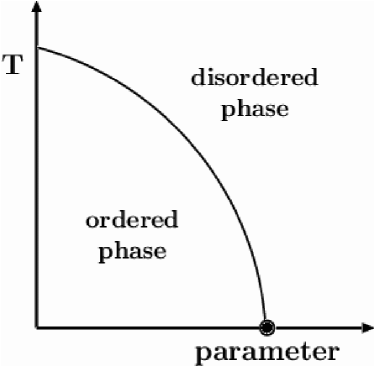
Figure 1: Schematic phase diagram near a Quantum Critical Point. The parameter along the $x$-axis can be quite general, like the pressure or a ratio of coupling constants. Whenever the critical temperature vanishes, a QCP, indicated with a dot in the figure, is encountered. In the vicinity of such a point quantum mechanical, zero-point fluctuations become very important. However when $T_{c}$ is finite, critical slowing down implies that the relevant frequency scale goes as $\omega\sim|T_{c}-T|^{\nu z}$, dwarfing quantum effects; the standard classical critical methodology then applies. An example of a phase diagram of this type for $MnSi$ is shown in Fig. 34 below.

The density-density correlations of itinerant disordered electrons at long wavelengths and low energies must have a diffusive form. In two-dimensions this leads to logarithmic singularities in the effective interactions when the interactions are treated perturbatively. The problem of finding the ground state and low-lying excitations in this situation is unsolved. On the experimental side the discovery of the metal-insulator transition in two dimensions and the unusual properties observed in the metallic state makes this an important problem to resolve.

The one-dimensional electron gas reveals logarithmic singularities in the effective interactions even in a second-order perturbation calculation. A variety of mathematical techniques have been used to solve a whole class of interacting one-dimensional problems and one now knows the essentials of the correlation functions even in the most general case. An important issue is whether and how this knowledge can be used in higher dimensions.

The solution of the Kondo problem and the realization that its low temperature properties may be discussed in the language of FLT has led in turn to the formulation and solution of impurity models with singular low energy properties. Such models have a QCP for a particular relation between the coupling constants; in some examples they exhibit a quantum critical line. The thermodynamic and transport properties around such critical points or lines are those of local singular Fermi-liquids. Although the direct experimental relevance of such models (as of one-dimensional models) to experiments is often questionable, these models, being soluble, can be quite instructive in helping to understand the conditions necessary for the breakdown of FLT and associated quasiparticle concepts. The knowledge from zero-dimensional and one-dimensional problems must nevertheless be used with care.

A problem which we do not discuss but which belongs in the study of SFL’s is the Quantum Hall Effect problem. The massive degeneracies of two-dimensional electrons in a magnetic-field leads to spectacular new properties and involves new fractional quantum numbers. The essentials of this problem were solved following Laughlin’s inspired variational calculation. The principal reason for the omission is firstly that excellent papers reviewing the developments are available [199, 71, 107] and secondly that the methodology used in this problem is in general distinct from those for discussing the other SFL’s which have a certain unity. We will however have occasions to refer to aspects of the quantum Hall effect problem often. Especially interesting from our point of view is the weakly singular Fermi-liquid behavior predicted in the $\nu=1/2$ Quantum Hall Effect [113].

One of the aspects that we want to bring to the foreground in this review is the fact that SFL’s all have in common some fundamental features which can be stated usefully in several different ways. (i) they have degenerate ground states to within an energy of order $k_{B}T$. This degeneracy is not due to static external potentials or constraints as in, for example the spin-glass problem, but degeneracies which are dynamically generated.(ii) Such degeneracies inevitably lead to a breakdown of perturbative calculations because they generate infra-red singularities in the correlation functions. (iii) If a bare particle or hole is added to the system, it is attended by a divergent number of low energy particle-hole pairs, so that the one-to-one correspondence between the one-particle excitation of the interacting problem and those of the non-interacting problem, which is the basis for FLT, breaks down.

On the theoretical side, one may now view Fermi-liquid theory as a forerunner of the Renormalisation Group ideas. The renormalisation group has led to a sophisticated understanding of singularities in the collective behavior of many-particle systems. Therefore these methods have an important role to play in understanding the breakdown of FLT.

The aim of this paper is to provide a pedagogical introduction to SFL’s, focused on the essential conceptual ideas and on issues which are settled and which can be expected to survive future developments. Therefore, we will not attempt to give an exhaustive review of the literature on this problem or of all the experimental systems which show hints of SFL behavior. The experimental examples we discuss have been selected to illustrate both what is essentially understood and what is not understood even in principle. On the theoretical side, we will shy away from presenting in depth the sophisticated methods necessary for a detailed evaluation of correlation functions near QCP — for this we refer to the book by Sachdev [210] — or for an exact solution of local impurity models (see, e.g., [118, 212, 244]). Likewise, for a discussion of the application of quantum critical scaling ideas to Josephson arrays or quantum Hall effects, we refer to the nice introduction by Sondhi et al. [232].

1.2 Outline of the paper

The outline of this paper is as follows. We start by summarizing in section 2 some of the key features of Landau’s FLT — in doing so, we will not attempt to retrace all of the ingredients which can be found in many of the classical textbooks [194, 36]; instead our discussion will be focused on those elements of the theory and the relation with its microscopic derivation that allow us to understand the possible routes in which the FLT can break down. This is followed in section 3 by the Fermi-liquid formulation of the Kondo problem and of the SFL variants of the Kondo problem and of two-interacting Kondo impurities. The intention here is to reinforce the concepts of FLT in a different context as well as to provide examples of SFL behavior which offer important insights because they are both simple and solvable. We then discuss the problem of one spatial dimension ($d=1$), presenting the principal features of the solutions obtained. We discuss why $d=1$ is special, and the problems encountered in extending the methods and the physics to $d>1$. We move then from the comforts of solvable models to the reality of the discussion of possible mechanisms for SFL behavior in higher dimensions. First we analyze in section 5 the paradigmatic case of long range interactions. Coulomb interactions will not do in this regard, since they are always screened in a metal, but transverse electromagnetic fields do give rise to long-range interactions. The fact that as a result no metal is a Fermi-liquid for sufficiently low temperatures was already realized long ago [120] — from a practical point of view this mechanism is not very relevant, since the temperatures where these effects become important are of order $10^{-16}$ Kelvin; nevertheless, conceptually this is important since it is a simple example of a gauge theory giving rise to SFL behavior. Gauge theories on lattices have been introduced to discuss problems of fermions moving with the constraint of only zero or single occupation per site. We then discuss in section 6 the properties near a quantum critical point, taking first an example in which the ferromagnetic transition temperature goes to zero as a function of some externally chosen suitable parameter. We refer in this section to several experiments in heavy fermion compounds which are only partially understood or not understood even in principle. We then turn to a discussion of the marginal Fermi-liquid phenemenology for the SFL state of copper-oxide High - $T_{c}$ materials and discuss the requirements on a microscopic theory that the phenemenology imposes. A sketch of a microscopic derivation of the phenemenology is also given. We close the paper in section 8 with a discussion of the metallic state in $d=2$ and the state of the theory treating the diffusive singularities in $d=2$ and its relation to the metal-insulator transition.

2 Landau’s Fermi-liquid

2.1 Essentials of Landau Fermi-liquids

The basic idea underlying Landau’s Fermi-liquid theory [144, 145, 194, 36] is that of analyticity, i.e. that states with the same symmetry can be adiabatically connected. Simply put this means that whether or not we can actually do the calculation we know that the eigenstates of the full Hamiltonian of the same symmetry can be obtained perturbatively from those of a simpler Hamiltonian. At the same time states of different symmetry can not be obtained by “continuation” from the same state. This suggests that given a hard problem which is impossible to solve, we may guess a right simple problem. The low energy and long wavelength excitations, as well as the correlation and the response functions of the impossible problem bear a one-to-one correspondence with the simpler problem in their analytic properties. This leaves fixing only numerical values. These are to be determined by parameters, the minimum number of which is fixed by the symmetries. Experiments often provide intuition as to what the right simple problem may be: for the interacting electrons, in the metallic range of densities, it is the problem of kinetic energy of particles with Fermi statistics (If one had started with the opposite limit, just the potential energy alone, the starting ground state is the Wigner crystal — a bad place to start thinking about a metal!). If we start with non-interacting fermions, and then turn on the interactions, the qualitative behavior of the system does not change as long as the system does not go through (or is close to) a phase transition. Because of the analyticity, we can even consider strongly interacting systems — the low energy excitations in these have strongly renormalized values of their parameters compared to the non-interacting problem, but their qualitative behavior is the same of that of the simpler problem.

The heavy fermion problem provides an extreme example of the domain of validity of the Landau approach. This is illustrated in Fig. 2, which shows the specific heat of the heavy fermion compound $CeAl_{3}$. As in the Sommerfeld model, the specific heat is linear in the temperature at low $T$, but if we write $C_{v}\approx\gamma T$ at low temperatures, the value of $\gamma$ is about a thousand times as large as one would estimate from the density of states of a typical metal, using the free electron mass. For a Fermi gas the density of states $N(0)$ at the Fermi energy is proportional to an effective mass $m^{*}$:

$$N(0)={{m^{*}k_{F}}\over{\pi^{2}\hbar^{2}}}~{},$$ (1)

with $k_{F}$ the Fermi wavenumber. Then the fact that the density of states at the chemical potential is a thousand times larger than for normal metals can be expressed by the statement that the effective mass $m^{*}$ of the quasiparticles is a thousand times larger than the free electron mass $m$. Likewise, as Fig. 3 shows, the resistivity of $CeAl_{3}$ at low temperatures increases as $T^{2}$. This also is a characteristic sign of a Fermi-liquid, in which the quasiparticle lifetime $\tau$ at the Fermi surface, determined by electron-electron interactions, behaves as $\tau\sim 1/T^{2}$. However, just as the prefactor $\gamma$ of the specific heat is a factor thousand times larger than usual, the prefactor of the $T^{2}$ term in the resistivity is a factor $10^{6}$ larger — while $\gamma$ scales linearly with the effective mass ratio $m^{*}/m$, the prefactor of the $T^{2}$ term in the resistivity increases for this class of Fermi-liquids as $(m^{*}/m)^{2}$.

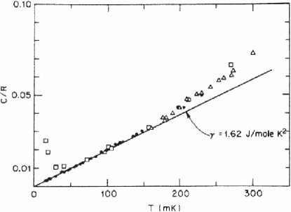
Figure 2: Specific heat of $CeAl_{3}$ at low temperatures from Andres et al. [28]. The slope of the linear specific heat is about 3000 times that of the linear specific heat of say $Cu$. But the high-temperature cut-off of this linear term is smaller than that of $Cu$ by a similar amount. The rise of the specific heat in a magnetic field at low temperatures is the nuclear contribution, irrelevant to our discussion.

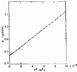
Figure 3: Electrical resistivity of $CeAl_{3}$ below 100 $mK$, plotted against $T^{2}$. From Andres et al. [28].

It should be remarked that the right simple problem is not always easy to guess. The right simple problem for liquid ${}^{4}He$ is not the non-interacting Bose gas but the weakly interacting Bose gas (i.e. the Bogoliubov problem [44, 146]). The right simple problem for the Kondo problem (a low-temperature local Fermi liquid) was guessed [184] only after the numerical renormalization group solution was obtained by Wilson [273]. The right simple problem for two-dimensional interacting disordered electrons in the ”‘metallic” range of densities (section 8 in this paper) is at present unknown.

For SFL’s the problem is different: usually one is in a regime of parameters where no simple problem is a starting point — in some cases the fluctuations between solutions to different simple problems determines the physical properties, while in others even this dubious anchor is lacking.

2.2 Landau Fermi-liquid and the wave function renormalization $Z$

Landau theory is the forerunner of our modern way of thinking about low-energy effective Hamiltonians in complicated problems and of the renormalisation group. The formal statements of Landau theory in their original form are often somewhat cryptic and mysterious — this both reflects Landau’s style and his ingenuity. We shall take a more pedestrian approach.

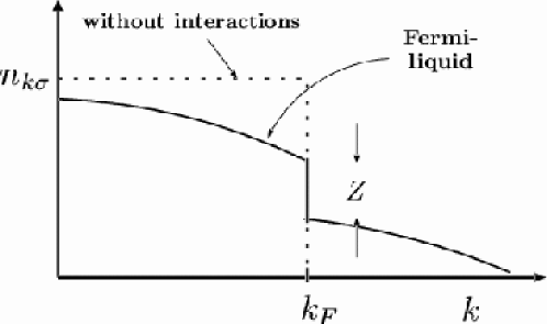
Figure 4: Bare-particle distribution at $T=0$ for a given spin-direction in a translationally invariant Fermi-system with interactions (full line) and without interactions (dashed line). Note that the position of the discontinuity, i.e. the Fermi wavenumber $k_{F}$, is not renormalized by interactions.

Let us consider the essential difference between non-interacting fermions and an interacting Fermi-liquid from a simple microscopic perspective. For free fermions, the momentum states $|{\bf k}\rangle$ are also eigenstates with energy eigenvalue

$$\epsilon_{\bf k}={{\hbar^{2}k^{2}}\over{2m}}$$ (2)

of the Hamiltonian. Moreover, the distribution of particles is given by the Fermi-Dirac function for the thermal occupation $n^{0}_{{\bf k}\sigma}$, where $\sigma$ denotes the spin label. At $T=0$ the distribution jumps from 1 (all states occupied within the Fermi sphere) to zero (no states occupied within the Fermi sphere) at$|{\bf k}|=k_{F}$ and energy equal to the chemical potential $\mu$. This is illustrated in Fig. 4.

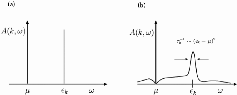
Figure 5: (a) The non-interacting spectral function $A(k,\omega)$ at fixed $k$ as a function of $\omega$. (b) The spectral function of single-electron excitations in a Fermi-liquid at fixed $k$ as a function of $\omega$. If $\frac{1}{\pi}A(k,\omega)$ is normalized to 1, signifying one bare particle, the weight under the Lorentzian, i.e. the quasi-particle part, is $Z$. As explained in the text, at the same time $Z$ is the discontinuity in Fig. 4.

A good way to probe a system is to investigate the spectral function; the spectral function $A(k,\omega)$ gives the distribution of energies $\omega$ in the system when a particle with momentum ${\bf k}$ is added or removed from it (Remember that removing a particle excitation below the Fermi energy means that we add a hole excitation). As sketched in Fig. 5(a), for the non-interacting system, $A_{0}({\bf k},\omega)$ is simply a delta-function peak at the energy $\epsilon_{\bf k}$, because all momentum states are also energy eigenstates:

$$A_{0}({\bf k},\omega) = \delta(\omega-(\epsilon_{\bf k}-\mu))~{},~{}~{}~{}\mbox{for}~{}\omega>\mu~{},$$ (3)

$$= -{{1}\over{\pi}}\mbox{Im}{{1}\over{\omega-(\epsilon_{\bf k}-\mu)+i\delta}}=-{{1}\over{\pi}}\mbox{Im}G^{0}({\bf k},\omega)~{}.$$ (4)

Here $\delta$ is small and positive; it reflects that particles or holes are introduced adiabatically, and is taken to zero at the end of the calculation for the pure non-interacting problem. The first step of the second line is just a simple mathematical rewriting of the delta function; in the second line the Green’s function $G^{0}$ for non-interacting electrons is introduced. More generally the single-particle Green’s function $G({\bf k},\omega)$ is defined in terms of the correlation function of particle creation and annihilation operators in standard textbooks [182, 4, 208, 159]. For our present purposes, it is sufficient to note that it is related to the spectral function $A({\bf k},\omega)$, which has a clear physical meaning and which can be deduced through Angle Resolved Photoemission Experiments :

$$G({\bf k},\omega)=\int_{-\infty}^{\infty}dx~{}{{A({\bf k},x)}\over{\omega-\mu-x+i\delta\>\mbox{sgn}(\omega-\mu)}}.$$ (5)

$A({\bf k},\omega)$ thus is the spectral representation of the complex function $G(k,\omega)$. Here we have defined the so-called ${\it retarded}$ Green’s function which is especially useful since its real and imaginary parts obey the Kramers-Kronig relations. In the problem with interactions $G({\bf k},\omega)$ will differ from $G^{0}({\bf k},\omega)$. This difference can be quite generally defined through the single-particle self-energy function $\Sigma({\bf k},\omega)$:

$$\left(G({\bf k},\omega)\right)^{-1}=\left(G^{0}({\bf k},\omega)\right)^{-1}-\Sigma({\bf k},\omega)~{}.$$ (6)

Eq. (5) ensures the relation between $G({\bf k},\omega)$ and $A({\bf k},\omega)$

$$A({\bf k},\omega)=-{{1}\over{\pi}}\mbox{Im}\;G({\bf k},\omega)~{}.$$ (7)

With these preliminaries out of the way, let us consider the form of $A({\bf k},\omega)$ when we add a particle to an interacting system of fermions.

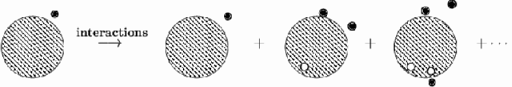
Figure 6: Schematic illustration of the perturbative expansion (8) of the change of wave function as a result of the addition of an electron to the Fermi sea due to interactions with the particles in the Fermi sea.

Due to the interaction (assumed repulsive) between the added particle and those already in the Fermi-sea, the added particle will kick particles from below the Fermi-surface to above. The possible terms in a perturbative description of this process are constrained by the conservation laws of charge, particle number, momentum and spin. Those which are allowed by the aforementioned conservation laws are indicated pictorially in Fig. 6, and lead to an expression of the type

$$|\psi^{N+1}_{{\bf k}\sigma}\rangle = Z_{{\bf k}}^{1/2}c_{{\bf k}\sigma}^{\dagger}|\psi^{N}\rangle+{{1}\over{V^{3/2}}}\sum_{{{\bf k}_{1},{\bf k}_{2},{\bf k}_{3}}}\sum_{\sigma_{1},\sigma_{2},\sigma_{3}}\alpha_{{\bf k}_{1}\sigma_{1}{\bf k}_{2}\sigma_{2}{\bf k}_{3}\sigma_{3}}c^{\dagger}_{{\bf k}_{3}}c_{{\bf k}_{2}}c^{\dagger}_{{\bf k}_{1}}~{}\times$$ (8)

$$\hskip 85.35826pt\times~{}\delta_{{\bf k},{\bf k}_{1}-{\bf k}_{2}+{\bf k}_{3}}\delta(\sigma;\sigma_{1},\sigma_{2},\sigma_{3})|\psi^{N}\rangle+\cdots~{}.$$

Here the $c^{\dagger}_{\bf k}$’s and $c_{\bf k}$’s are the bare particle creation and annihilation operators, and the dots indicate higher order terms, for which two or more particle-hole pairs are created and $\delta(\sigma;\sigma_{1},\sigma_{2},\sigma_{3})$ expresses conservation of spin under vector addition. The multiple-particle-hole pairs for a fixed total momentum can be created with a continuum of momentums of the individual bare particles and holes. Therefore an added particle with fixed total momentum has a wide distribution of energies. However if $Z_{\bf k}$ defined by Eqn. (8) is finite, there will be a well-defined feature in this distribution at some energy which is in general different from the non-interacting value $\hbar^{2}k^{2}/(2m)$. The spectral function in such a case will then be as illustrated in Fig. 5. It is useful to separate the well-defined feature from the broad continuum by writing the spectral function as the sum of two terms, $A({\bf k},\omega)=A_{coh}({\bf k},\omega)+A_{incoh}({\bf k},\omega)$. The single-particle Green’s function can be expressed as a sum of two corresponding terms, $G({\bf k},\omega)=G_{coh}({\bf k},\omega)+G_{incoh}({\bf k},\omega)$. Then

$$G_{coh}({\bf k},\omega)={{Z_{\bf k}}\over{\omega-\tilde{\epsilon}_{\bf k}+i/\tau_{\bf k}}}~{},$$ (9)

which for large lifetimes $\tau_{\bf k}$ gives a Lorentzian peak in the spectral density at the quasiparticle energy $\tilde{\epsilon}_{\bf k}\equiv\epsilon_{\bf k}-\mu$. The incoherent Green’s function is smooth and hence for large $\tau_{\bf k}$ corresponds to the smooth background in the spectral density.

The condition for the occurrence of the well-defined feature can be expressed as the condition on the self-energy $\Sigma({\bf k},\omega)$ that it has an analytic expansion about $\omega=0$ and ${\bf k}={\bf k}_{F}$ and that its real part be much larger than its imaginary part. One can easily see that were it not so the expression (9) for $G_{coh}$ could not be obtained. These conditions are necessary for a Landau Fermi-liquid. Upon expanding $\Sigma({\bf k},\omega)$ in (12) for small $\omega$ and small deviations of ${\bf k}$ from ${\bf k}_{F}$ and writing it in the form (9), we make the identifications

$$\tilde{\epsilon}_{\bf k}=\epsilon_{\bf k}Z_{\bf k}\hat{Z}_{\bf k}~{},~{}~{}~{}~{}~{}~{}~{}~{}{{1}\over{\tau_{\bf k}}}=Z_{\bf k}\>\mbox{Im}\Sigma({\bf k}_{F},\omega=0)~{},$$ (10)

where

$$Z_{\bf k}=\left(1-{{\partial\Sigma}\over{\partial\omega}}\right)_{\omega=0,k=k_{F}}^{-1}~{},~{}~{}~{}~{}~{}~{}~{}~{}~{}~{}\hat{Z}=\left(1+{{1}\over{v_{F}}}{{\partial\Sigma}\over{\partial k}}\right)_{\omega=0,k=k_{F}}~{}.$$ (11)

From Eq. (8) we have a more physical definition of $Z_{\bf k}$: $Z_{\bf k}$ is the projection amplitude of $|\psi_{{\bf k}}^{N+1}\rangle$ onto the state with one bare particle added to the ground state, since all other terms in the expansion vanish in the thermodynamic limit in the perturbative expression embodied by (8),

$$Z_{\bf k}^{1/2}=\langle\psi_{\bf k}^{N+1}|c^{\dagger}_{\bf k}|\psi^{N}\rangle~{}.$$ (12)

In other words, $Z_{\bf k}$ is the overlap of the ground state wavefunction of a system of interacting $N\pm 1$ fermions of total momentum ${\bf k}$ with the wave function of $N$ interacting particles and a bare-particle of momentum ${\bf k}$. $Z_{\bf k}$ is called the quasiparticle amplitude.

The Landau theory tacitly assumes that $Z_{\bf k}$ is finite. Furthermore it asserts that for small $\omega$ and ${\bf k}$ close to ${\bf k}_{F}$, the physical properties can be calculated from quasiparticles which carry the same quantum numbers as the particles, i.e. charge, spin and momentum and which may be defined simply by the creation operator $\gamma^{\dagger}_{{\bf k},\sigma}$:

$$|\psi^{N+1}_{\bf k}\rangle=\gamma^{\dagger}_{\bf k}|\psi^{N}\rangle~{}.$$ (13)

Close to ${\bf k}_{F}$, and for $T$ small compared to the Fermi-energy, the distribution of the quasiparticles is assumed to be the Fermi-Dirac distribution in terms of the renormalized quasiparticle energies. The bare particle distribution is quite different. As is illustrated in Fig. 4, it is depleted below ${\bf k}_{F}$ and augmented above ${\bf k}_{F}$, with a discontinuity at $T=0$ whose value is shown in microscopic theory to be $Z_{\bf k}$. A central result of Fermi-liquid theory is that close to the Fermi energy at zero temperature, the width $1/\tau_{\bf k}$ of the coherent quasiparticle peak is proportional to $(\epsilon_{\bf k}-\mu)^{2}$ so that near the Fermi energy the lifetime is long and quasiparticles are well-defined. Likewise, at the Fermi energy $1/\tau_{\bf k}$ varies with temperature as $T^{2}$. From the microscopic derivation of this result, it follows that the weight in this peak, $Z_{\bf k}$, becomes equal to the jump $Z$ in $n_{{\bf k}\sigma}$ when we approach the Fermi surface: $Z_{\bf k}{\rightarrow Z}$ for ${{\bf k}\rightarrow{\bf k}_{F}}$. For heavy fermions, as we already mentioned, $Z$ can be of the order of $10^{-3}$. But as long as $Z$ is nonzero, one has Fermi-liquid properties for temperatures lower than about $ZE_{F}$. Degeneracy is effectively lost for temperatures much higher than $ZE_{F}$ and classical statistical mechanics prevails.

An additional result from microscopic theory is the so-called Luttinger theorem, which states that the volume enclosed by the Fermi-surface does not change due to interactions [182, 4]. The mathematics behind this theorem is that with the assumptions of FLT, the number of poles in the interacting Green’s function below the chemical potential is the same as that for the non-interacting Green’s function. Recall that the latter is just the number of particles in the system.

Landau actually started his discussion of the Fermi-Liquid by writing the equation for the deviation of the (Gibbs) free-energy from its ground state value as a functional of the deviation of the quasiparticle distribution function $n({\bf k},\sigma)$ from the equilibrium distribution function $n_{0}({\bf k},\sigma)$

$$\delta n({\bf k},\sigma)=n({\bf k},\sigma)-n_{0}({\bf k},\sigma),$$ (14)

as follows:

$$G=G_{0}+{{1}\over{V}}\sum_{{\bf k},\sigma}(\epsilon_{\bf k}-\mu)\delta n_{{\bf k}\sigma}+{{1}\over{2V^{2}}}\sum_{{\bf k}{\bf k}^{\prime},\sigma\sigma^{\prime}}f_{{\bf k}{\bf k}^{\prime},\sigma\sigma^{\prime}}\delta n_{{\bf k}\sigma}\delta n_{{\bf k}^{\prime}\sigma^{\prime}}+\cdots$$ (15)

Note that $(\epsilon_{\bf k}-\mu)$ is itself a function of $\delta n$; so the first term contains at least a contribution of order $(\delta n)^{2}$ which makes the second term quite necessary. In principle, the unknown function $f_{{\bf k}{\bf k}^{\prime},\sigma\sigma^{\prime}}$ depends on spin and momenta. However, spin rotation invariance allows one to write the spin part in terms of two quantities, the symmetric and antisymmetric parts $f^{s}$ and $f^{a}$. Moreover, for low-energy and long-wavelength phenomena only momenta with ${\bf k}\approx{\bf k}_{F}$ play a role; if we consider the simple case of ${}^{3}He$ where the Fermi surface is spherical, rotation invariance implies that for momenta near the Fermi momentum $f$ can only depend on the relative angle between ${\bf k}$ and ${\bf k}^{\prime}$; this allows one to expand in Legendre polynomials $P_{l}(x)$ by writing

$$N(0)f^{s,a}_{{\bf k}{\bf k}^{\prime},\sigma\sigma^{\prime}}\stackrel{{\scriptstyle{\bf k}\approx{\bf k}^{\prime}\approx{\bf k}_{F}}}{{\longrightarrow}}\sum_{l=0}^{\infty}F_{l}^{s,a}P_{l}(\hat{{\bf k}}\cdot\hat{{\bf k}}^{\prime})~{}.$$ (16)

From the expression (15) one can then relate the lowest order so-called Landau coefficients $F_{0}$ and $F_{1}^{s}$ and the effective mass $m^{*}$ to thermodynamic quantities like the specific heat $C_{v}$, the compressibility $\kappa$, and the susceptibility $\chi$:

$${{C_{v}}\over{C_{v0}}}={{m^{*}}\over{m}}~{},~{}~{}~{}~{}~{}{{\kappa}\over{\kappa_{0}}}=(1+F^{s}_{0}){{m^{*}}\over{m}}~{},~{}~{}~{}~{}~{}{{\chi}\over{\chi_{0}}}=(1+F^{a}_{0}){{m^{*}}\over{m}}~{}.$$ (17)

Here subscripts 0 refer to the quantities of the non-interacting reference system, and $m$ is the mass of the fermions. For a Galilean invariant system (like ${}^{3}He$), there is a a simple relation between the mass enhancement and the Landau parameter $F^{s}_{1}$, and there is no renormalization of the particle current ${\bf j}$; however, there is a renormalization of the velocity: one has

$${\bf j}={\bf k}/m~{},~{}~{}~{}~{}~{}~{}~{}{\bf v}={\bf k}/m^{*}~{},~{}~{}~{}~{}~{}~{}~{}{{m^{*}}\over{m}}=\left(1+{{F^{s}_{1}}\over{3}}\right)~{}.$$ (18)

The transport properties are calculated by defining a distribution function $\delta n({\bf k}\sigma;r,t)$ which is slowly varying in space and time and writing a Boltzmann equation for it [194, 36].

It is a delightful conceit of the Landau theory that the expressions of the low-energy properties in terms of the quasiparticles in no place involve the quasiparticle amplitude $Z_{\bf k}$. In fact in a translationally invariant problem as liquid ${}^{3}He$, $Z_{\bf k}$ cannot be measured by any thermodynamic or transport measurements . A masterly use of conservation laws ensures that $Z$’s cancel out in all physical properties (One can extract $Z$ from measurement of the momentum distribution. By neutron scattering measurements, it is found that $Z\approx 1/4$ [108] for $He^{3}$ near the melting line). This is no longer true on a lattice, in the electron-phonon interaction problem [198] or in heavy fermions [250] or even more generally in any situation where the interacting problem contains more than one type of particle with different characteristic frequency scales.

2.3 Understanding microscopically why Fermi-liquid Theory works

Let us try to understand from a more microscopic approach why the Landau theory works so well. We present a qualitative discussion in this subsection and outline the principal features of the formal derivation in the next subsection.

As we already remarked, a crucial element in the approach is to choose the proper non-interacting reference system. That this is possible at all is due to the fact that the number of states to which an added particle can scatter due to interactions is severely limited due to the Pauli principle. As a result non-interacting fermions are a good stable system to perturb about: they have a finite compressibility and susceptibility in the ground state, and so collective modes and thermodynamic quantities change smoothly when the interactions are turned on. This is not true for non-interacting bosons which do not support collective modes like sound waves. So one cannot perturb about the non-interacting bosons as a reference system.

Landau also laid the foundations for the formal justification of Fermi Liquid theory in two and three dimensions. The flurry of activity in this field following the discovery of high-$T_{c}$ phenomena has led to new ways of justifying Fermi-liquid theory (and understanding why the one-dimensional problem is different). But the principal physical reason, which we now discuss, remains the phase space restrictions due to kinematical constraints.

We learned in section 2.2 that to be able to define quasiparticles, it was necessary to have a finite $Z_{{\bf k}_{F}}$ and that this in turn needed a self-energy function $\Sigma({{\bf k}_{F},\omega})$ which is smooth near the chemical potential, i.e. at $\omega=0$. Let us first see why a Fermi gas has such properties when interactions are calculated perturbatively.

In Fig. 7 we show the three possible processes that arise in second order perturbation theory for the scattering of two particles with fixed initial energy $\omega$ and momentum $q$. Note that in two of the diagrams, Fig. 7(a) and 7(b) the intermediate state has a particle and a hole while the intermediate state in diagram 7(c) has a pair of particles.

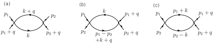
Figure 7: The three second-order processes in a perturbative calculation of the correction to the bare interaction in a Fermi-liquid

We will find that, for our present purpose, the contribution of diagram 7(a) is more important than the other two. It gives a contribution

$$g^{2}\sum_{\bf k}{{f_{\bf k+q}-f_{\bf k}}\over{\omega-(E_{\bf k+q}-E_{\bf k})+i\delta}}~{}.$$ (19)

Here $g$ is a measure of the strength of the scattering potential (the vertex in the diagram) in the limit of small ${\bf q}$. The denominator ensures that the largest contribution to the scattering comes from small scattering momenta ${\bf q}$: for these the energy difference is linear in ${\bf q}$, $E_{{\bf k}+{\bf q}}-E_{\bf k}\approx{\bf q}\cdot{\bf v_{\bf k}}$, where ${\bf v_{\bf k}}$ is a vector of length $v_{F}$ in the direction of ${\bf k}$. Moreover, the term in the numerator is nonzero only in the area contained between two circles (for $d=2$) or spheres (for $d=3$) with their centers displaced by ${\bf q}$ — here is the phase space restriction due to the Pauli principle! This area is also proportional to ${\bf q}\cdot{\bf v_{k}}$, and so in the small ${\bf q}$ approximation we get from diagram 7(a) a term proportional to

$$g^{2}{{{\bf q}\cdot{\bf v_{\bf k}}}\over{\omega-{\bf q}\cdot{\bf v_{\bf k}}+i\delta}}~{}{{df}\over{d\epsilon_{\bf k}}}~{}.$$ (20)

Now we see why we diagram 7(a) is special. There is a singularity at $\omega={\bf q\cdot v_{k}}$ and its value for small $\omega$ and ${\bf q}$ depends on which of the two is smaller. This singularity is responsible for the low energy-long wavelength collective modes of the Fermi liquid in Landau theory. At low temperatures, $df/d\epsilon_{\bf k}=-\delta(\epsilon_{\bf k}-\mu)$, so the summation is restricted to the Fermi surface. The real part of (19) therefore vanishes in the limit $qv_{F}/\omega\rightarrow 0$, while it approaches a finite limit for $\omega\rightarrow 0$. The imaginary part in this limit is proportional to $\omega$,

$$Im\chi({\bf q},\omega)=g^{2}\pi N(0){{\omega}\over{qv_{F}}}~{}~{}~{}~{}\mbox{for}~{}\omega<qv_{F}~{},$$ (21)

while $Im\chi({\bf q},\omega)=0$ for $\omega>v_{F}q$. This behavior is sketched in Fig. 8(b). Explicit evaluation yields for the real part

$$Re\chi({\bf q},\omega)=g^{2}N(0)\left[1+\frac{\omega}{qv_{F}}\ln\left|\frac{\omega-qv_{F}}{\omega+qv_{F}}\right|\>\right]~{},$$ (22)

which gives a constant (leading to a finite compressibility and spin susceptibility) at $\omega$ small compared to $qv_{F}$. For diagram 7(b), we get a term $\omega-(E_{\bf{p_{1}-p_{2}+k+q}}-E_{\bf k})$ in the denominator. This term is always finite for general momenta ${\bf p_{1}}$ and ${\bf p}_{2}$, and hence the contribution from this diagram can always be neglected relative to the one from 7(a). Along similar lines, one finds that diagram 7(c), which describes scattering in the particle-particle channel, is irrelevant except when ${\bf p}_{1}=-{\bf p}_{2}$, when it diverges as $\ln\omega$.

Of course, this scattering process is the one which gives superconductivity. Landau noticed this singularity but ignored its implication. Indeed, as long as the effective interactions do not favor superconductivity or as long as we are at temperatures much higher than the superconducting transition temperature, it is not important for Fermi-liquid theory.

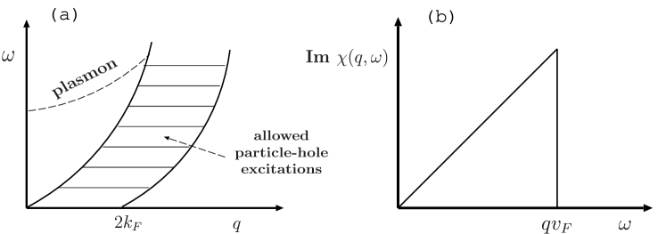
Figure 8: (a) Restriction on allowed particle-hole excitations in a Fermi-sea due to kinematics. The plasmon mode has been drawn for the case $d=3$. (b) The absorptive part of the particle-hole susceptibility (in the charge, current and spin channels) for $\omega<qv_{F}$ in the Fermi gas.

Let us now look further at the absorptive spectrum of particle-hole excitations in two and three dimensions, i.e., we examine the imaginary part of Eq. (19). When the total energy $\omega$ of the pair is small, both the particle and the hole have to live close to the Fermi surface. In this limit, we can make any excitation with momentum $q\leq 2k_{F}$. For fixed but small values of $q$, the maximum excitation energy is $\omega\approx qv_{F}$; this occurs when ${\bf q}$ is in the same direction as the main momentum ${\bf k}$ of each quasiparticle. For $q$ near $2k_{F}$ the maximum possible energy is $\omega=v_{F}|q-2k_{F}|$. Combining these results, we get the sketch in Fig. 8(a), in which the shaded area in the $\omega$-$q$ space is the region of allowed particle-hole excitations. From this spectrum one can calculate the polarizability, or the magnetic susceptibility.

The behavior sketched above is valid generally in two and three dimensions (but as we will see in section 4, not in one dimension). The important point to remember is that the density of particle-hole excitations decreases linearly with $\omega$ for $\omega$ small compared to $qv_{F}$. We shall see later that one way to undo Fermi-liquid theory is to have $\omega$ vary as $k^{2}$ in two dimensions or $\omega\sim k^{3}$ in three dimensions.

We can now use $\mbox{Im}\;\chi({\bf q},\omega)$ to calculate the single-particle self-energy to second order in the interactions. This is shown in Fig. 9 where the wiggly line denotes $\chi({\bf q},\nu)$ which in the present approximation is just given by the diagram of Fig. 7(a).

For the perturbative evaluation of this process, the intermediate particle with energy-momentum $(\omega+\nu)$, $(k+q)$ is a free particle. Second order perturbation theory then yields an imaginary part or decay rate

$$\mbox{Im}\,\Sigma({\bf k},\omega)={{1}\over{\tau({\bf k},\omega)}}=g^{2}N(0)\left({{\omega}\over{E_{F}}}\right)^{2}~{},$$ (23)

in three dimensions for ${\bf k}\approx{\bf k}_{F}$. In two dimensions, the same process yields $\mbox{Im}\,\Sigma({\bf k}_{F},\omega)\sim\omega^{2}\ln(E_{F}/\omega)$.

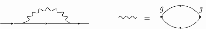
Figure 9: The single-particle self-energy diagram in second order.

The $\omega^{2}$ decay rate is intimately related to the analytic result (22) for $\mbox{Im}~{}\chi(q,\omega)$ exhibited in Fig. (8). As may be found in text books, the same calculation for electron-phonon interactions or for interaction with spin waves in an antiferromagnetic metal gives $\mbox{Im}\,\Sigma({\bf k}_{F},\omega)\sim(\omega/\omega_{c})^{3}$, with $\omega_{c}$ is the phonon Debye frequency in the former and the characteristic zone-boundary spin-wave frequency in the latter.

The real part of the self-energy may be obtained directly or by Kramers–Kronig transformation of (23). It is proportional to $\omega$. Therefore, if the quasiparticle amplitude $Z_{k_{F}}$ is evaluated perturbatively

$$Z_{k_{F}}\approx 1-2g^{2}N(0)/E_{F}~{}.$$ (24)

Thus in a perturbative calculation of the effect of interactions the basic analytic structure of the Green’s function is left the same as for non-interacting fermions. The general proof of the validity of Landau theory consists in showing that what we have seen in second order in $g$ remains true to all orders in $g$. The original proofs [4] are self-consistency arguments — we will consider them briefly in section 2.4. They assume a finite $Z$ in exact single-particle Green’s functions and show effectively that to any order of perturbation, the polarizability functions retain the analytic structure of the non-interacting theory, which in turn ensures a finite $Z$.

In one dimension, phase space restrictions on the possible excitations are crucially different, since the Fermi surface consists of just two points in the one-dimensional space of momenta — see Fig. 10. As a result, whereas in $d=2$ and $d=3$ a continuum of low-energy excitations with finite $q$ is possible, at low energy only excitations with small $k$ or $k\approx 2k_{F}$ are possible. The subsequent equivalence of Fig. 8 for the one-dimensional case is the one shown in Fig. 11. Upon integrating over the momentum $k$ with a cut-off of ${\cal{O}}(k_{F})$ the contribution from this particle-hole scattering channel to $\mbox{Re}\,\chi(q,\omega)$ is

$$\int dk{{1}\over{\omega+(2k+q)v_{F}}}\sim\ln[(\omega+qv_{F})/E_{F}]~{}.$$ (25)

(Note that (25) is true for both $q<<k_{F}$ and $|q-2k_{F}|<<k_{F}$.) This in turn leads to a single particle self-energy calculated by the process in Fig. 9 to be $\mbox{Re}\,\Sigma({\bf k}_{F},\omega)\sim\omega\ln\omega$ giving a hint of trouble. Also the Cooper (particle-particle) channel has the same phase space restrictions, and gives a contribution also proportional to $\ln\omega$. The fact that these sngular contributions are of the same order, leads to a competition between charge/spin fluctuations and Cooper pairing fluctuations, and to power law singularities. Also, the fact that instead of a continuum of low energy excitations as in higher dimensions, the width of the band of allowed particle hole excitations vanishes as $\omega\rightarrow 0$, is the reason that the properties of one-dimensional interacting metals can be understood in terms of bosonic modes. We will present a brief summary of the results for the single-particle Green’s function and correlation functions in section 4.9.

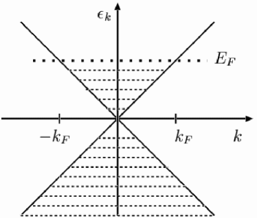
Figure 10: Single-particle energy $\epsilon_{k}$ in one dimension, in the approximation that the dispersion relation is linearized about $k_{F}$. Note the Fermi surface consists of just two points. The spectrum of particle-hole excitations is given by $\omega(q)=\epsilon(k+q)-\epsilon(k)=k_{F}q/m$. Low-energy particle-hole excitations are only possible for $q$ small or for $q$ near $2k_{F}$.

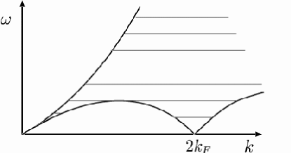
Figure 11: Phase space for particle-hole excitation spectrum in one dimension. Compare with the same in higher dimensions, Fig. 8. For linearized single-particle kinetic energy $\epsilon_{k}=\pm v_{F}(k-k_{F})$, particle-hole excitations are only possible on lines going through $k=0$ and $k=2k_{F}$.

In special cases of nesting in two or three dimensions, one can have situations that resemble the above one-dimensional case. When the non-interacting Fermi surface in a tight binding model has the square shape sketched in Fig. 12(a) — this happens for a tight-binding model with nearest neighbor hopping on a square lattice at half-filling — a continuous range of momenta on opposite sides of the Fermi surface can be transformed into each other by one and the same wavenumber. This so-called nesting leads to $\log$ and $\log^{2}$ singularities for a continuous range of ${\bf k}$ in the perturbation theory for the self energy $\Sigma({\bf k},\omega)$. Likewise, the partially nested Fermi surface of Fig. 12(b) leads to charge density wave and antiferromagnetic instabilities. We will come back to these in sections 2.6 and 6.

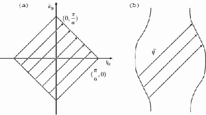
Figure 12: (a) The nested Fermi surface on obtained in a tight binding model on a square lattice with nearest neighbor hopping; (b) A partially nested Fermi surface which leads to charge density wave or antiferromagnetic instabilities

2.4 Principles of the Microscopic Derivation of Landau Theory

In this section we will sketch how the conclusions in the previous section based on second-order perturbation calculation are generalized to all orders in perturbation theory. This section is slightly more technical than the rest; the reader may choose to skip to section 2.6.

We follow the microscopic approach whose foundations were laid by Landau himself and which is discussed in detail in excellent textbooks [184, 194, 36, 4]. For more recent methods with the same conclusions see [222, 121]. Our emphasis will be on highlighting the assumptions in the theory so that in the next section we can summarize the routes by which the Fermi-liquid theory may break down. These assumptions are usually not stated explicitly.

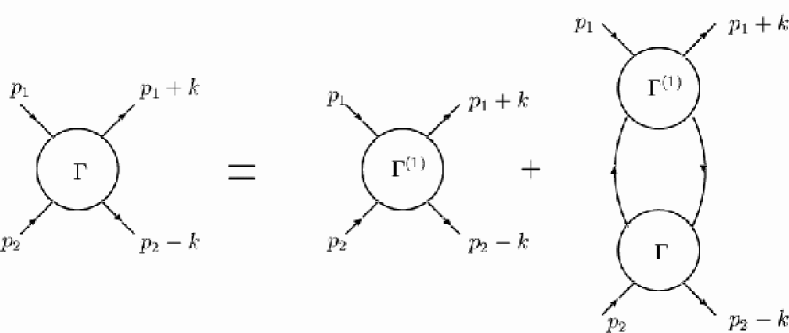
Figure 13: Diagrammatic representation of Eq. (27).

The basic idea is that due to kinematic constraints, any perturbative process with $n$ particle-hole pairs in the intermediate state gives contributions to the polarizability proportional to $(\omega/E_{F})^{n}$. Therefore the low energy properties can be calculated with processes with the same “skeletal” structure as those in Fig. 7, which have only one particle-hole pair in the intermediate state. So one may concentrate on the modification of the four-legged vertices and the single-particle propagators due to interactions to all orders. Accordingly the theory is formulated in terms of the single particle Green’s function $G(p)$ and the two-body scattering vertex,

$$\Gamma\left(p_{1},\ p_{2},\ p_{1}\ +\ k,\ p_{2}\ -k\right)\ =\Gamma\left(p_{1},\ p_{2},\ k\right)$$ (26)

Here and below we use, for sake of brevity, $p$, etc. to denote the energy-momentum four-vector $({\bf p},\omega)$ and we suppress the spin labels. The equation for $\Gamma$ is expanded in one of the two particle-hole channels as

$$\Gamma(p_{1},p_{2},k)\ = \ \Gamma^{(1)}(p_{1},p_{2},k)$$ (27)

$$~{}~{}~{}-i\smallint\ \Gamma^{(1)}(p_{1},q,k)\ G(q)G(q+k)\ \Gamma(q,p_{2},k){d^{4}q\over(2\pi)^{4}}\ ,$$

where $\Gamma^{(1)}$ is the irreducible part in the particle hole channel in which Eq. (27) is expressed. In other words, $\Gamma^{(1)}$ can not be split up into two parts by cutting two Green’s function lines with total momentum $k$. So $\Gamma^{(1)}$ includes the complete vertex in the other (often called cross-) particle-hole channel. The diagrammatic representation of Eq. (27) is shown in Fig. 13. In the simplest approximation $\Gamma^{(1)}$ is just the bare two-body interaction. Landau theory assumes that $\Gamma^{(1)}$ has no singularities An assumption is now further made that $G(p)$ does have a coherent quasiparticle part at $|{\bf p}|\simeq p_{F}$ and $\omega\simeq 0$,

$$G(p)={{Z}\over{\omega-\tilde{\epsilon}_{\bf p}+i\delta\>\mbox{sgn}(\epsilon_{\bf p})}}\ +\ G_{inc}~{},$$ (28)

where $\tilde{\epsilon}_{\bf p}$ is to be identified as the excitation energy of the quasiparticle, $Z$ its weight, and $G_{inc}$ the non-singular part of $G$ (The latter provides the smooth background part of the spectral function in Fig. 5(b) and the former the sharp peak, which is proportional to the $\delta$ function for $\tilde{\epsilon}_{\bf p}=\epsilon_{\bf p}-\mu$. It follows [182, 4] from (28) that

$$G(q)G(q+k)\ =\ {2i\pi z^{2}\over v_{F}}\ {{{\bf v_{q}}\cdot{\bf k}}\over{\omega-{\bf v_{q}}\cdot{\bf k}}}\delta(\nu)\delta(|{\bf q}|-p_{F})+\phi(q)~{},$$ (29)

for small ${\bf k}$ and $\omega$, and where $\nu$ and $(\nu+\omega)$ are frequencies of the two Green’s functions. Note the crucial role of kinematics in the form of the first term which comes from the product of the quasiparticle parts of $G$; $\phi(q)$ comes from the scattering of the incoherent part with itself and with the coherent part and is assumed smooth and featureless (as it is indeed, given that $G_{inc}$ is smooth and featureless and the scattering does not produce an infrared singularity at least perturbatively in the interaction). The vertex $\Gamma$ in regions close to ${\bf k}\approx{\bf k}_{F}$ and $\omega\approx 0$ is therefore dominated by the first term. The derivation of Fermi-liquid theory consists in proving that the equations (27) for the vertex and (28) for the Green’s function are mutually consistent.

The proof proceeds by defining a quantity $\Gamma^{\omega}(p_{1},p_{2},k)$ through

$$\Gamma^{\omega}\left(p_{1},p_{2},k\right)\ = \ \Gamma^{(1)}(p_{1},p_{2},k)$$ (30)

$$~{}~{}~{}-i\smallint\ \Gamma^{(1)}(p_{1},q,k)\phi(q)\ \Gamma^{\omega}(q,p_{2},k)\ {d^{4}q\over(2\pi)^{4}}~{}.$$

$\Gamma^{\omega}$ contains repeated scattering of the incoherent part of the particle-hole pairs among itself and with the coherent part, but no scattering of the coherent part with itself. Then, provided the irreducible part of $\Gamma^{(1)}$ is smooth and not too large, $\Gamma^{\omega}$ is smooth in $k$ because $\phi(q)$ is by construction quite smooth.

Using the fact that the first part of (29) vanishes for $v_{F}|k|/\omega\rightarrow 0$, and comparing (27) and (30) one can write the forward scattering amplitude

$$\lim_{\omega\rightarrow 0}\>\left[\lim_{k\rightarrow 0}\ \Gamma(p_{1},p_{2},k)\right]\ =\ \Gamma^{\omega}(p_{1},p_{2})\ .$$ (31)

This is now used to write the equation for the complete vertex $\Gamma$ in terms of $\Gamma^{\omega}$:

$$\Gamma(p_{1},p_{2},k) = \Gamma^{\omega}(p_{1},p_{2})$$ (32)

$$~{}~{}~{}+{Z^{2}p_{F}^{2}\over(2\pi)^{3}v_{F}}\ \int\ \Gamma^{\omega}(p_{1},q)\Gamma(q,p_{2},k){{{\bf v_{q}}\cdot{\bf k}}\over{\omega-{\bf v_{q}}\cdot{\bf k}}}d\Omega_{q}~{},$$

where in the above $|q|=p_{F}$ and one integrates only over the solid angle $\Omega_{q}$.

Given a non-singular $\Gamma^{\omega}$, a non-singular $\Gamma$ is produced (unless the denominator in Eq. (32) produces singularities after the indicated integration-the Landau-Pomeranchuk singularities discussed below). The one-particle Green’s function $G$ can be expressed exactly in terms of $\Gamma$ — see Fig. 14. This leads to Eq. (28) proving the self-consistency of the ansatz with a finite quasiparticle weight $Z$. The quantity $Z^{2}\Gamma^{\omega}$ is then a smooth function and goes into the determination of the Landau parameters.

The Landau parameters can be written in terms of the forward scattering amplitude. In effect they parametrize the momentum and frequency independent scattering of the incoherent parts among themselves and with the coherent parts so that the end result of the theory is that the physical properties can be expressed purely in terms of the quasiparticle part of the single-particle Green’s function and the Landau parameters. No reference to the incoherent parts needs to be made for low energy properties. For single-component translational invariant fermions (like liquid ³He) even the quasiparticle amplitude $Z$ disappears from all physical properties. This last is not true for renormalization due to electron-phonon interactions and in multi-component systems such as heavy fermions. Special simplifications of the Landau theory occur in such problems and in other problems where the single-particle self-energy is nearly momentum independent [168, 264, 101, 250, 175].

As we also mentioned, the single-particle self-energy $\Sigma$ can be written exactly in terms of the vertex $\Gamma$: the relation between the two is represented diagrammatically in Fig. 14. The relations between $\Sigma$ and $\Gamma$ are due to conservation laws which Landau theory, of course, obeys. But the conservation laws are more general than Landau theory. It is often more convenient to express these conservation laws as relations between the self-energy and the three-point vertices, $\Lambda_{\alpha}(p\epsilon;q\omega)$ which couple external perturbations to either the density (the fourth component, $\alpha=4$) or the current density in the $\alpha=(1,2,3)$ direction The diagrammatic representation of the equation for $\Lambda$ is shown in Fig. 15. The following relations (Ward identities) have been proven for translationally invariant problems:

$$\lim\left({\epsilon\over q}\rightarrow 0,\ q\rightarrow 0\right)\Lambda_{\alpha}({\bf p}\epsilon;{\bf q}\omega) = {p_{\alpha}\over m}-{\partial\over\partial p_{\alpha}}\Sigma({\bf p},\epsilon)~{},~{}~{}~{}~{}(\alpha=1,2,3)$$ (33)

$$\lim\left({\epsilon\over q}\rightarrow 0,\ q\rightarrow 0\right)\Lambda_{4}({\bf p}\epsilon;{\bf q}\omega) = 1+{{\partial\Sigma({\bf p},\epsilon)}\over{\partial\epsilon}}~{},$$ (34)

$$\lim\left({q\over\epsilon}\rightarrow 0,\epsilon\rightarrow 0\right)\Lambda_{\alpha}({\bf p}\epsilon;{\bf q}\omega) = {p_{\alpha}\over m}-{d\over dp_{\alpha}}\Sigma({\bf p},\epsilon)~{},~{}~{}~{}~{}(\alpha=1,2,3)$$ (35)

$$\lim\left({q\over\epsilon}\rightarrow 0,\epsilon\rightarrow 0\right)\Lambda_{4}({\bf p}\epsilon;{\bf q}\omega) = 1+{d\Sigma({\bf p},\epsilon)\over d\mu}~{}.$$ (36)

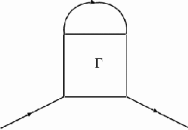
Figure 14: Diagram for the exact single-particle self-energy in terms of the exact vertex $\Gamma$ and the exact single-particle Green’s function.

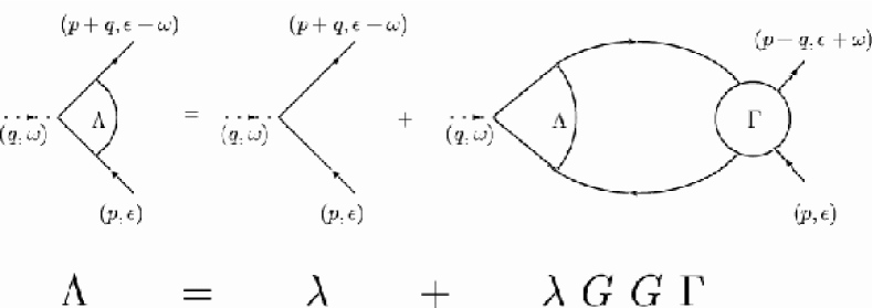
Figure 15: Vertex for coupling to external perturbations at energy-momentum $(\omega,q)$; $\lambda$ is the bare vertex.

A relation analogous to (34) is derived for fields coupling to spin for the case that interactions conserve spin. The total derivative in (35) and (36) [rather than the partial derivative in (33) and (34)] represents that $d\Sigma/d\mu$ is the variation in $\Sigma$ when $\epsilon$ is changed to $\epsilon+d\epsilon$ together with $\mu$ to $\mu+d\mu$, and $d\Sigma/dp_{\alpha}$ represents the variation when the momentum ${\bf p}$ as well as the Fermi-surface is translated by $dp_{\alpha}$.

Eq. (36) is an expression of energy conservation, and Eq. (34) of particle number conservation. Eqs. (33) and (34) together signify the continuity equation. Eq. (35) represents current conservation.

In Landau theory, the right hand sides in Eqs. (33)-(36) are expressible in terms of the Landau parameters. These relations are necessary to derive the renormalization in the various thermodynamic quantities that we quoted in Eqs. (17) and (18) as well as the Landau transport equation. Needless to say, any theory of SFL must also be consistent with the Ward identities.

2.5 Modern derivations

The modern derivations of Fermi-liquid theory start as well by assuming the existence of a Fermi surface. Kinematics then inevitably leads to similar considerations as above. Instead of the division into coherent and incoherent part made in Eq. (28), the renormalization group procedures are used to systematically generate a successively lower energy and small momentum Hamiltonian with excitations of particle ever closer to the Fermi surface. The calculations are done either in terms of fermions [222] or newly developed bosonization methods in arbitrary dimensions [121]. The end result is equivalent to Eqs. (28), (30) and (32). These methods may well turn out to be very important in finding the structure of SFL’s and in systematizing them.

These derivations do the calculation in arbitrary dimension $d$ and conclude that the forward scattering amplitude is

$$\Gamma^{\omega}(p_{1},p_{2},k)\ \sim\ \left({k\over k_{F}}\right)^{d-1}f(p_{1},p_{2},k)\ ,\$$ (37)

where $f$ is a smooth function of all of its arguments. In one-dimension the forward scattering amplitude has a logarithmic singularity, as we noted earlier.

We can rephrase the conceptual framework of Landau Fermi-liquid theory in the modern language of Renormalization Group theory [222]. As we discussed, in Fermi-Liquid theory one treats a complicated strongly interacting fermion problem by writing the Hamiltonian ${\mathcal{H}}$ as

$${\mathcal{H}}={\mathcal{H}}_{simple}+{\mathcal{H}}_{rest}~{}.$$ (38)

In our discussion ${\mathcal{H}}_{simple}$ was the non-interacting Hamiltonian. The non-interacting Hamiltonian is actually a member of a ’line’ of fixed-point Hamiltonians ${\mathcal{H}}^{*}$ all of which have the same symmetries but differ in their Landau parameters $F_{l}^{s,a}$ etc. The $F_{l}$’s, obtained from the forward scattering in Landau theory are associated with marginal operators and distinguish the properties of the various systems associated with the line of fixed points. Landau fermi-liquid theory is first of all the statement of the domain of attraction of this line of fixed points. The theory also establishes the universal low temperature properties due to the ”irrelevant” operators generated by ${\mathcal{H}}_{rest}$ due to scattering in channels other than the forward channel. Landau theory does not establish (at least completely) the domain of attraction of the ”critical surface” bounding the domain of attraction of the Fermi-liquid fixed line from those of other fixed points or lines. If ${\mathcal{H}}_{rest}$ were to generate a ”relevant” operator — i.e., effective interactions which diverge at low energies (temperatures) — the scheme breaks down. For example, attractive interactions between fermions generate relevant operators–they presage a transition to superconductivity, a state of different symmetry. But if we stay sufficiently above $T_{c}$, we can usually continue using Landau theory.

2.6 Routes to Breakdown of Landau Theory

From Landau’s phenomenological theory, one can only say that the theory breaks down when the physical properties — specific heat divided by temperature, compressibility, or the magnetic susceptibility — diverge or when the collective modes representing oscillations of the Fermi-surface in any harmonic and singlet or triplet spin combinations become unstable. The latter, called the Landau-Pomeranchuk singularities, are indeed one route to the breakdown of Landau theory and occur when the Landau parameters $F_{l}^{s,a}$ reach the critical value $-(2l+1)$. A phase transition to a state of lower symmetry in then indicated. The new phase can again be described in Landau theory by defining distribution functions consistent with the symmetry of the new ground state.

The discussion following Eq. (8) in section 2.2 allows us to make a more general statement. Landau theory breaks down when the quasiparticle amplitude $Z_{\bf k}$ becomes zero; i.e. when the state $c_{\bf k}^{\dagger}|\psi^{N}\rangle$ and $|\psi_{\bf k}^{N+1}\rangle$ are orthogonal. This can happen if the series expansion in Eq. (8) in terms of the number of particle-hole pairs is divergent. In other words, addition of a particle or a hole to the system creates a divergent number of particle-hole pairs in the system so that the leading term does not have a finite weight in the thermodynamic limit. From Eq. (11) connecting the $Z^{\prime}s$ to $\Sigma^{\prime}s$, this requires that the single-particle self-energy be singular as a function of $\omega$ at $k\simeq k_{F}$. This in turn means that the Green’s functions of SFL’s contain branch cuts rather than the poles unlike Landau Fermi-liquids. The weakest singularity of this kind is encountered in the borderline “marginal Fermi-liquids” where

$$\Sigma(k_{F},\omega)\simeq\lambda\left[\omega\ln\frac{\omega_{c}}{\omega}+i|\omega|\right].$$ (39)

If a divergent number of low-energy particle-hole pairs is created upon addition of a bare particle, it means that the low-energy response functions (which all involve creating particle-hole pairs) of SFL’s are also divergent. Actually the single-particle self-energy can be written in terms of integrals over the complete particle-hole interaction vertex as in Fig. 14. The implication is that the interaction vertices are actually more divergent than the single-particle self-energy.

Yet another route to SFL’s is the case in which the interactions generate new quantum numbers which are not descriptive of the non-interacting problem. This happens most famously in the Quantum Hall problems and in one-dimensional problems (section 4) as well as problems of impurity scattering with special symmetries (section 3). In such cases the new quantum numbers characterize new low-energy topological excitations. New quantum numbers of course imply $Z=0$, but does $Z=0$ imply new quantum numbers. One might wish to conjecture that this is so. But there is no proof of this.

In the final analysis all breakdowns of Landau theory are due to degeneracies leading to singular low-energy fluctuations. If the characteristic energy of the fluctuations is lower than the temperature, a quasi-classical statistical mechanical problem results. On the basis of our qualitative discussion in section 2.3 and the sketch of the microscopic derivation in section 2.4, we may divide up the various routes to breakdown of Landau theory into the following (not necessarily orthogonal) classes:

(i) Landau-Pomeranchuk Singularities: Landau theory points to the possibility of its breakdown through the instability of the collective modes of the Fermi-surface which arise from the solution of the homogeneous part of Eqn.(32). These collective modes can be characterized by the angular momentum $\ell$ of oscillation of the Fermi-surface and whether the oscillation is symmetric “$s$” or anti-symmetric “$a$” in spin. The condition for the instability derived from the condition of zero frequency of the collective modes are [194, 36]

$$\matrix{F_{\ell}^{s}\leq-(2\ell+1)~{},~{}~{}~{}~{}~{}~{}F_{\ell}^{a}\leq-(2\ell+1)}~{}.$$ (40)

The $\ell=0$ conditions refer to the divergence in the compressibility and the (uniform) spin-susceptibility. The former would in general occur via a first-order transition, so is uninteresting to us. The latter describes the ferromagnetic instability. No other Landau-Pomeranchuk instabilities have been experimentally identified. But such new and exotic possibilities should be kept in mind. Thus, for example, an $F_{1}^{s}$-instability corresponds to the Fermi-velocity $\rightarrow 0$, a $F_{2}^{s}$ instability to a “$d$-$wave$-like” instability of the particle-hole excitations on the Fermi-surface etc. Presumably these instabilities are resolved by reconstruction of the Fermi-surface with (patches) of energy gaps. Coupling of the damped transverse-excitations of charged-fermions to zero-point fluctuations of the electromagnetic-fields produces an SFL which we study in section 5.1. The microscopic interactions necessary for the Landau-Pomeranchuk instabilities and the critical properties near such instabilities have not been well investigated, especially for fermions with a lattice potential.

It is also worth noting that some of the instabilities are disallowed in the limit of translational invariance. Thus, for example, time-reversal breaking states, such as the “anyon-state” [148, 59] cannot be realized because in a translationally invariant problem the current operator cannot be renormalized by the interactions, as we have learnt from Eqs. (18), (33).

(ii) Critical regions of Large Q-Singularities: Landau theory concerns itself only with long wavelength response and correlations. A Fermi-liquid may have instabilities at a nonzero wave-vector, for example a charge-density wave (CDW) or spin-density wave (SDW) instability. Only a microscopic calculation can provide the conditions for such instabilities and therefore such conditions can only be approximately derived. An important point to note is that they arise perturbatively from repeated scattering between the quasiparticle parts of $G$ while the scattering vertices (irreducible interactions)are regular. The superconductive instability for any angular momentum is also an instability of this kind. In general such instabilities are easily seen in RPA and/or $t$-matrix calculations.

Singular Fermi-liquid behavior is generally expected to occur only in the critical regime of such instabilities [112, 156]. If the transition temperature $T_{c}$ is finite then there is usually a stable low temperature phase in which unstable modes are condensed to an order parameter, translational symmetry is broken, and gaps arise in part or all of the Fermi-surface. For excitations on the surviving part of the Fermi-surface, Fermi-liquid theory is usually again valid. The fluctuations in the critical regime are classical, i.e. with characteristics frequency $\omega_{f\ell}\ll k_{B}T_{c}$.

If the transition is tuned by some external parameter so that it occurs at zero temperature, one obtains, as illustrated already in Fig. 1, a Quantum Critical Point (QCP). If the transition is approached at $T=0$ as a function of the external parameter, the fluctuations are quantum-mechanical, while if it is approached as a function of temperature for the external parameter at its critical value, the fluctuations have a characteristic energy proportional to the temperature. A large region of the phase diagram near QCP’s often carries SFL properties. We shall discuss such phenomena in detail in section 6.

(iii) Special Symmetries: The Cooper instability at $q=0$, Fig. 7(c), is due to the “nesting” of the Fermi-surface in the particle-particle channel. Usually indications of finite $q$-CDW or SDW singularities are evident pertubatively from Fig. 7(a) or Fig. 7(b) for special Fermi-surfaces, nested in some ${\bf q}$-direction in particle-hole channels. One-dimensional fermions are perfectly nested in both particle-hole channels and particle-particle channels (Figs. 7(a)-(c)) and hence they are both logarithmically singular. Pure one-dimensional fermions also have the extra conservation law that right going and left going momenta are separately conserved. These introduce special features to the SFL of one-dimensional fermions such as the introduction of extra quantum numbers. These issues are discussed in section 4.9. Several soluble impurity problems with special symmetries have SFL properties. Their study can be illuminating and we discuss them in section 3.

(iv) Long-Range Interactions: Breakdown of Landau Fermi-liquid may come about through long-range interactions, either in the bare Hamiltonian through the irreducible interaction or through a generated effective interaction. The latter, of course, happens in the critical regime of phase transitions such as discussed above. Coulomb interactions will not do for the former because of screening of charge fluctuations. The fancy way of saying this is that the longitudinal electromagnetic mode acquires mass in a metal. The latter is not true for current fluctuations or transverse electromagnetic modes which due to gauge invariance must remain massless. This is discussed in section 5.1, where it is shown that no metal at low enough temperature is a Fermi-liquid. However, the cross-over temperature is too low to be of experimental interest.

An off-shoot of an SFL through current fluctuations is the search for extra (induced) conservation laws for some quantities to keep their fluctuations massless. This line of investigation may be referred to generically as gauge theories. Extra conservation laws imply extra quantum numbers and associated orthogonality. We discuss these in section 5.2. The one-dimensional interacting electron problem and the Quantum Hall effect problems may be usefully thought of in these terms.

(v) Singularities in the Irreducible Interactions: In all the possibilities discussed in (i)-(iii) above the irreducible interactions $\Gamma^{(1)}$ defined after Eq. (27)are regular and not too large. As noted after Eq. (30) this is necessary to get a regular $\Gamma^{\omega}$. When these conditions are satisfied the conceivable singularities arise only from the repeated scattering of low-energy particle-hole (or particle-particle) pairs) as in Eq. (32) or its equivalent for large momentum transfers.

A singularity in the irreducible interaction of course invalidates the basis of Landau theory. Such singularities imply that the parts of the problem considered harmless perturbatively because they involve the incoherent and high energy parts of the single-particle spectral weight as in Eq. (30) are, in fact, not so. This is also true if $\Gamma^{(1)}$ is large enough that the solution of Eq. (30) is singular. Very few investigations of such processes exist.

How can an irreducible interaction be singular when the bare interaction is perfectly regular? We know of two examples:

In disordered metals the density correlations are diffusive with characteristic frequency $\omega$ scaling with $q^{2}$. The irreducible interactions made from the diffusive fluctuations and interactions are singular in $d=2$. This gives rise to a new class of SFL’s which are discussed in section 8. One finds that in this case the singularity in the cross-particle-hole channel (the channel different from the one through which the irreducibility of $\Gamma^{(1)}$ is defined) feeds back into a singularity in $\Gamma^{(1)}$. This is very special because the cross-channel is integrated over and the singularity in it must be very strong for this to be possible.

The second case concerns the particle singularities in the irreducible interactions because of excitonic singularities. Usually the excitonic singularities due to particle-hole between different bands occur at a finite energy and do not introduce low energy singularities. But if the interactions are strong enough these singularities occur near zero frequency. In effect eliminating high energy degrees of freedom generates low energy irreducible singular vertices.

Consider, for example, the band-structure of a solid with more than one atom per unit cell with (degenerate) valence band maxima and minima at the same points in the Brillouin zone, as in Fig. (16) .

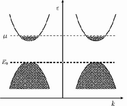
Figure 16: A model band structure for a solid with more than one atom per unit cell. Actually in $CaB_{6}$ where excitonic singularities have been invoked to produce a ferromagnetic state [280] there are three equivalent points in the Brillouin zone where the conduction band minima and the valence band maxima occur.

Let the conduction band be partially filled, and the energy difference between $\mu$ and the valence band marked $E_{0}$ in Fig. 16 be much smaller than the attractive particle-hole interactions $V$ between states in the valence (v) band and the conduction band (c). For any finite $V$ excitonic resonances form from scattering between $v$ and $c$ states, as in the $X$-ray edge problem to be discussed in section 3.5. For large enough $V$ such resonances occur at asymptotically low energy so that the Fermi-liquid description of states near the chemical potential in terms of irreducible interaction among the $c$-states is invalid. The effective irreducible interactions among the low-energy states integrate over the excitonic resonance and will in general be singular if the resonance is near zero-energy.

Such singularities require interactions above a critical magnitude and are physically and mathematically of an unfamiliar nature. In a 2-band one-dimensional model, exact numerical calculations have established the importance of such singularities [237, 234].

Recently it has been found that $CaB_{6}$ or $SrB_{6}$ with low density of trivalent $Eu$ or quadrivalent $Ce$ ions substituting for ($Ca$, $Sr$) is a ferromagnet [280]. The most plausible explanation [288, 33, 35] is that this is a realization of the excitonic ferromagnetism predicted by Volkov et al. [263]. The instability to such a state occurs because the energy to create a hole in the valence band and a particle in the conduction band above the fermi-energy goes to zero if the attractive particle-hole (interband)interactions are large enough. This problem has been investigated only in the mean-field approximation. Fluctuations in the critical regime of such a transition are well worth studying.

Excitonically induced singularities in the irreducible interactions are also responsible for the Marginal Fermi-liquid state of Cu$-$O metals in a theory to be discussed in section 7.

3 Local Fermi-Liquids & Local Singular Fermi-Liquids

In this section we discuss a particular simple form of Fermi-liquid formed by electrons interacting with a dilute concentration of magnetic impurity. Many of the concepts of Fermi-liquid theory are revisited in this problem. Variants of the problem provide an interesting array of soluble problems of SFL behavior and illustrate some of the principal themes of this article.

3.1 The Kondo Problem

The Kondo problem is at the same time one of the simplest and one of the most subtle examples of the effects of strong correlation effects in electronic systems. The experiments concern metals with a dilute concentration of magnetic impurities. In the Kondo model one considers only a single impurity; the Hamiltonian then is

$${\mathcal{H}}=t\sum_{\langle ij\rangle}c_{i\alpha}^{\dagger}c_{j\alpha}+J{\bf S}\cdot c_{0}^{\dagger}{\bf\sigma}c_{0}~{},$$ (41)

where $(c_{i\alpha},c_{i\alpha}^{\dagger})$ denote the annihilation and creation operators of a conduction electron at site $i$ with projection $\alpha$ in the $z$-direction of spin $\sigma$. The second term is the exchange interaction between a single magnetic impurity at the origin (with spin ${S}=1/2$) and a conduction electron spin.

When the exchange constant $J>0$ the system is a Fermi-liquid. Although not often discussed, the ferromagnetic ($J<0$) variant of this problem is one of the simplest examples of a singular Fermi-liquid.

There are two seemingly simple starting points for the problem: (i) $J=0$: This turns out to describe the unstable high temperature fixed point. The term proportional to $J$ is a marginal operator about the high temperature fixed point because as discovered by Kondo[138] in a third order perturbation calculation, the effective interaction acquires a singularity $\sim J^{3}/t^{2}\ln(t/\omega)$. (ii) $t=0$: The perturbative expansion about this point is well behaved. This turns out to describe the low temperature Fermi-liquid fixed point. One might be surprised by this, considering that typically the bare $t/J$ is of order $10^{+3}$. But such is the power of singular renormalizations.

The interaction between conduction electrons and the localized electronic level is not a direct spin interaction. It originates from quantum-mechanical charge fluctuations that (through the Pauli principle) depend on the relative spin orientation. To see this explicitly it is more instructive to consider the Anderson model [19] in which

$${\mathcal{H}} = t\sum_{\langle ij\rangle}c_{i\alpha}^{\dagger}c_{j\alpha}+\epsilon_{d}\sum_{\sigma}c_{0\sigma}^{\dagger}c_{0\sigma}+Uc_{0,\uparrow}^{\dagger}c_{0,\uparrow}c_{0,\downarrow}^{\dagger}c_{0,\downarrow}+$$ (42)

$$\hskip 85.35826pt+\sum_{k,\sigma}(V_{k}c_{k,\sigma}^{\dagger}c_{0,\sigma}+h.c.)$$

The last term in this Hamiltonian is the hybridization between the localized impurity state and the conduction electrons, in which spin is conserved. In the particle-hole symmetric case, $\epsilon_{d}=-U/2$ is the one-hole state on the impurity site in the Hartree-Fock approximation and the one-particle state has the energy $U/2$.

Following a perturbative treatment in the limit $\frac{t}{V},\frac{U}{V}\gg 1$ the Anderson model reduces to the Kondo Hamiltonian with an effective exchange constant $J_{eff}\sim(V^{2}/t)^{2}/U$.

The Anderson model has two simple limits, which are illustrated in Fig. 17:

(i) $V=0$: This describes a local moment with Curie susceptibility $\chi\sim\mu_{B}^{2}/T$. This limit is the correct point of departure for an investigation for the high temperature regime. As noted one soon encounters the Kondo divergences.

(ii) $U=0$: In this limit the impurity forms a resonance of width $\Gamma\sim V^{2}/t$ at the chemical potential which in the particle-hole symmetric case is half-occupied. The ground state is a spin singlet. This limit is the correct starting point for an examination of the low temperature properties ($T\ll T_{K}$). A temperature independent contribution to the susceptibility and a linear contribution to the specific heat ($\sim N(0)T/\Gamma$) are contributed by the resonant state. Hence the name local Fermi-Liquid.

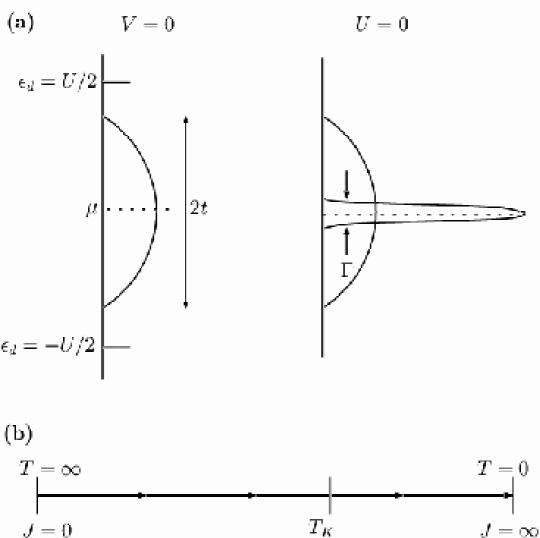
Figure 17: (a) Hartree-Fock excitation spectrum of the Anderson model in the two limits of zero hybridization, $V=0$ and zero interaction, $U=0$. (b) Renormalization group flow of the Kondo problem.

The conceptually hard part of the problem was to realize that (ii) is the correct stable low temperature fixed point and the technically hard problem is to derive the passage from the high-temperature regime to the low-temperature regime. This was first done correctly by Wilson [273] through the invention of the Numerical Renormalization Group (and almost correctly by Anderson and Yuval [22, 23] by analytic methods). The analysis showed that under Renormalization Group scaling transformations the ratio $(J/t)$ increases monotonically as illustrated in Fig. 17(b) — continuous RG flows are observed from the high temperature extreme (i) to the low temperature extreme (ii) and a smooth crossover between between the two regimes occurs at the Kondo temperature

$$T_{K}\sim t\exp(-t/2J).$$ (43)

Because all flow is towards the strong-coupling fixed point, universal forms for the thermodynamic functions are found. For example, the specific heat $C_{v}$ and the susceptibility $\chi$ scale as

$$C_{v}=Tf_{c}(T/T_{K}),~{}~{}~{}~{}~{}~{}~{}~{}~{}~{}~{}~{}\chi=\mu_{B}^{2}f_{\chi}(T/T_{K})~{},$$ (44)

where the $f$’s are universal scaling functions.

An important theoretical result is that compared to a non-interacting resonant level at the chemical potential, the ratio of the magnetic susceptibility enhancement to the specific heat enhancement,

$$R_{W}={{\delta\chi/\chi}\over{\delta C_{v}/C_{v}}}$$ (45)

for spin 1/2 impurities at $T\ll T_{K}$ is precisely 2 [273, 184]. In a noninteracting model, this ratio, nowadays called the Wilson ratio, is equal to 1, since both $\chi$ and $C_{v}$ are proportional to the density of states $N(0)$. Thus the Wilson ratio is a measure of the importance of correlation effects. It is in fact the analogue of the Landau parameter $F_{0}^{a}$ of Eq. (18).

3.2 Fermi-liquid Phenemenology for the Kondo problem

Following Wilson’s solution [273], Nozières [184] showed that the low-temperature properties of the Kondo problem can be understood simply through a (local) Fermi-liquid framework. This is a beautiful example of the application of the concept of analyticity and of symmetry principles about a fixed point. We present the key arguments below. For the application of this line of approach to the calculation of a variety of properties we refer the reader to papers by Nozières and Blandin [184, 185].

The properties of a local impurity can be characterized by the energy-dependent $s$-wave phase shift $\delta_{\sigma}(\epsilon)$, which in general also depends on the spin of the conduction electron being scattered. In the spirit of Fermi-liquid theory the phase shift may be written in terms of the deviation of the distribution function $\delta n(\epsilon)$ of conduction electrons from the equilibrium distribution,

$$\delta_{\sigma}(\epsilon)=\delta_{0}(\epsilon)+\sum_{\epsilon^{\prime}\sigma^{\prime}}\delta_{\sigma\sigma^{\prime}}(\epsilon,\epsilon^{\prime})\delta n_{\sigma^{\prime}}(\epsilon^{\prime})+...~{}.$$ (46)

About a stable fixed point the energy dependence is analytic near the chemical potential $(\epsilon=0)$, so that we may expand

$$\delta_{0}(\epsilon)=\delta_{0}+\alpha\epsilon+...~{},~{}~{}~{}~{}~{}~{}~{}~{}\delta_{\sigma\sigma^{\prime}}(\epsilon,\epsilon^{\prime})=\phi_{\sigma\sigma^{\prime}}+...~{}.$$ (47)

Just as the Landau parameters are expressed in terms of symmetric and antisymmetric parts, we can write

$$\phi_{\uparrow\uparrow}=\phi_{\downarrow\downarrow}=\phi^{s}+\phi^{a}~{},~{}~{}~{}~{}~{}~{}~{}~{}~{}~{}~{}~{}~{},~{}\phi_{\downarrow\uparrow}=\phi_{\uparrow\downarrow}=\phi^{s}-\phi^{a}~{}.$$ (48)

Taken together, this leaves three parameters $\alpha$, $\phi^{s}$ and $\phi^{a}$ to determine the low-energy properties. Nozières [184] showed that in fact there is only one independent parameter (say $\alpha$ which is of ${\mathcal{O}}(1/T_{K})$, with a prefactor which can be obtained by comparing with Wilson’s detailed numerical solution). To show this note that by the Pauli principle same spin states do not interact, therefore [184]

$$\phi_{\uparrow\uparrow}=\phi^{s}+\phi^{a}=0~{}.$$ (49)

Secondly a shift of the chemical potential by $\delta\mu$ and a simultaneous increase in $\delta n$ by $N(0)\delta\mu$ should have no effect on the phase shift, since the Kondo-effect is tied to the chemical potential. Therefore according to 46) and (47)

$$[\alpha+N(0)\phi^{s}]\delta\mu=0~{},~{}~{}~{}~{}~{}\Longrightarrow\phi^{s}=-\alpha/N(0)~{}.$$ (50)

Thirdly, one may borrow from Wilson’s solution that the fixed point has $\delta_{0}=\pi/2$. This expresses that the tightly bound spin singlet state formed of the impurity spin and conduction electron spin completely blocks the impurity site to other conduction electrons; this in turn implies maximal scattering and phase shift of $\pi/2$ for the effective scattering potential [184]. In other words, it is a strong-coupling fixed-point where one conduction electron state is pushed below the chemical potential in the vicinity of the impurity to form a singlet resonance with the impurity spin. One may now calculate all physical properties in term of $\alpha$. In particular, one finds $\delta C_{v}/C_{v}=2\alpha/(\pi VN(0)$ and a similar expression for the enhancement of $\chi$,such that the Wilson ratio of 2.

3.3 Ferromagnetic Kondo problem and the anisotropic Kondo problem

The ferromagnetic Kondo problem provides us with the simplest example of SFL behavior. We will discuss this below after relating the problem to a general $X$-ray edge problem in which the connection to the so-called orthogonality catastrophe is clearer. As discussed in Sec.2, orthogonality plays an important role in SFLs generally.

we start with the anisotropic generalization of the Kondo Hamiltonian, which is the proper starting model for a perturbative scaling analysis [21, 98],

$$H = t\sum_{\langle ij\rangle,\sigma}c_{i\sigma}^{\dagger}c_{j\sigma}+\sum_{k,k^{\prime}}\left[J_{\pm}\left(S^{+}c_{k\downarrow}^{\dagger}c_{k^{\prime}\uparrow}+S^{-}c_{k\uparrow}^{\dagger}c_{k^{\prime}\downarrow}\right)\right.+$$ (51)

$$\hskip 85.35826pt+J_{z}S^{z}\left.\left(c_{k,\uparrow}^{\dagger}c_{k^{\prime},\uparrow}-c_{k,\downarrow}^{\dagger}c_{k^{\prime},\downarrow}\right)\right]~{}.$$

Long before the solution of the Kondo problem, perturbative Renormalization Group for the effective vertex coupling constants $J_{\pm}$ and $J_{z}$ as a function of temperature were obtained [21, 98]. The scaling relation between them is found to be exact to all orders in the $J^{\prime}s$:

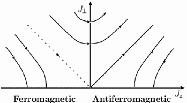
Figure 18: Renormalization group flows for the Kondo problem, displaying the line of critical points for the “ferromagnetic” problem and the flow towards the fixed point $J^{*}_{\pm}=J^{*}_{z}\to\infty$ for the “antiferromagnetic” problem.

$$(J_{z}^{2}-J_{\pm}^{2})=\mbox{const,}~{}~{}~{}~{}~{}(J_{+}=J_{-})~{}.$$ (52)

In the flow diagram 18 we show the scaling trajectories for the anisotropic problem. In the antiferromagnetic regime the flows continuously veer towards larger and larger $(J_{\pm},J_{z})$ values; at the resulting fixed point $(J*_{\pm},J*_{z})=(\infty,\infty)$ singlets form between the local moment and the conduction electrons.

The ’ferromagnetic’ regime spans the region satisfying the inequalities $J_{z}<0$ and $|J_{z}|\geq J_{\pm}$. Upon reducing the bandwidth the coupling parameters flow towards negative $J_{z}$ values. Observe the line of fixed points on the negative $J_{z}$ axis. Such a continuous line is also seen in the Kosterlitz-Thouless transition [139] of the two-dimensional XY model. Moreover, in both problems continuously varying exponents in physical properties are obtained along these lines (in fact, the renormalization group flow equations of the Kondo model for small coupling are mathematically identical to those for the XY model). This is an instance of a zero temperature Quantum Critical line. The physics of the Quantum Critical line has to do with an ”Orthogonality Catastrophe” which we describe next. Such orthogonalities are an important part of the physics of SFL’s generally.

3.4 Orthogonality Catastrophe

As we saw in section 2, a Fermi-liquid description is appropriate so long as the spectrum retains a coherent single particle piece of finite weight $Z>0$. So if by some miracle the evaluation of $Z$ reduces to an overlap integral between two orthogonal wave functions then the system is a SFL.

In the thermodynamic ($N\rightarrow\infty$) limit, such a miracle is more generic than might appear at first sight. In fact, such an orthogonality catastrophe arises if the injection of an infinitely massive particle in more than one dimension produces an effective finite range scattering potential for the remaining $N$ electrons [20] (see Sec.(4.9). Such an orthogonality is exact only in the thermodynamic limit: The single particle wave functions are not orthogonal. It is only the overlap between the ground state formed by their Slater determinantswhich vanishes as $N$ tends to infinity.

More quantitatively, if the injection of the additional particle produces an $s$-wave phase shift $\delta_{0}$ for the single particle wave functions (all $N$ of them),

$$\phi(kr)=\frac{\sin kr}{kr}\rightarrow\frac{\sin(kr+\delta_{0})}{kr}$$ (53)

then an explicit computation of the Slater determinants reveals that their overlap diminishes as

$$\langle\psi_{N}|\psi_{N}^{\prime}\rangle\sim N^{-\delta_{0}^{2}/\pi^{2}}.$$ (54)

Here $|\psi_{N}\rangle$ is the determinant Fermi sea wave function for $N$ particles and $|\psi_{N}^{\prime}\rangle$ is the wavefunction of the system after undergoing a phase shift by the local perturbation produced by the injected electron.

Quite generally such an orthogonality ($Z=0$) arises also if two $N$ particle states of a system possess different quantum numbers and almost the same energy. These new quantum numbers might be associated with novel topological excitations. This is indeed the case in the Quantum Hall Liquid where new quantum numbers are associated with fractional charge excitations. The SFL properties of the interacting one-dimensional fermions (Section 4) may also be looked on as due to orthogonality. Often orthogonality has the effect of making a quantum many-body problem approach the behavior of a classical problem. This will be one of the leitmotifs in this review. We turn first to a problem where this orthogonality is well understood to lead to experimental consequences, although not at low energies.

3.5 X-ray Edge singularities

The term $X$-ray edge singularity is used for the line shape for absorption in metals by creating a hole in an atomic core-level and a particle in the conduction band above the chemical potential. In the non-interacting particle description of this process, the absorption starts at the threshold frequency $\omega_{D}$, as sketched in Fig. 19. In this case, a Fermi edge reflecting the density of unoccupied states in the conduction band is expected to be visible the spectrum.

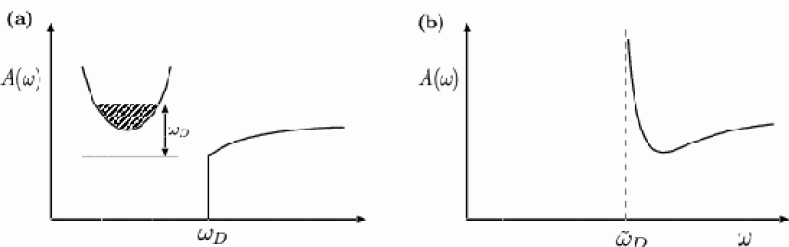
Figure 19: Absorption lineshape for transitions between a lower dispersionless level and a conduction band, (a) for zero interaction between the conduction electrons and local level, and (b) for small interaction.

However, when a hole is generated in the lower level, the potential that the conduction electrons see is different. The relevant Hamiltonian is now

$${\mathcal{H}}=\epsilon_{d}\left(d^{\dagger}d-\frac{1}{2}\right)+\sum_{k}\epsilon_{k}c_{k}^{\dagger}c_{k}+\frac{1}{L}\sum_{k,k^{\prime}}V(k,k^{\prime})\left(c_{k}^{\dagger}c_{k^{\prime}}-\frac{1}{2}\right)\left(d^{\dagger}d-\frac{1}{2}\right)~{},$$ (55)

where spin indices have been suppressed. The operators $(d,d^{\dagger})$ annihilate or create holes in the core level, which is taken to be dispersionless. The first two terms in the Hamiltonian represent the unperturbed energies of the core hole and the free electrons. The last term depicts the screened Coulomb interaction between the conduction electrons and the hole in the core level.

As a consequence of the interactions, the line shape is quite different. This is actually an exactly solvable problem [183]. There are two kinds of effects, (a) excitonic — the particle and the hole attract, leading to a shift of the edge and a sharpening of the edge singularity — and (b) an orthogonality effect of the type just discussed above, which smoothens the edge irrespective of the sign of the interaction. This changes the absorption spectrum to that of Fig. 19(b) in the presence of interactions. The form of the singularity is [158, 183]

$$A(\omega)\sim(\omega-\tilde{\omega}_{D})^{-2\frac{\delta_{0}}{\pi}+\frac{\delta_{0}^{2}}{\pi^{2}}}.$$ (56)

The exponent $\delta_{0}^{2}/\pi^{2}$ is a consequence of the orthogonality catastrophe overlap integral; the exponent $(-2\delta_{0}/\pi)$ is due to the excitonic particle hole interactions. If the hole has finite mass we have a problem with recoil which is not exactly solvable, but we know the essential features of the solution. As we will discuss later in section 4.9, recoil removes the singularity in two and three dimensions and the absorption edge acquires a characteristic width of the order of the dispersion of the hole band. If the hole moves only in one dimension, the singularity is not removed.

3.6 A Spinless Model with Finite Range Interactions

A model, which is a generalization of the Ferromagnetic Kondo problem and in which the low-energy physics is dominated by the orthogonality catastrophe, is given by the following Hamiltonian :

$${\mathcal{H}}=\sum_{k,l}\epsilon_{k}\gamma_{k,l}^{\dagger}\gamma_{k,l} + \frac{t}{\sqrt{L}}\sum_{k}(\gamma_{k,0}^{\dagger}d+h.c.)$$ (57)

$$~{}~{}~{}+\frac{1}{L}\sum_{k,k^{\prime}}V_{l}\left(\gamma_{k,l}^{\dagger}\gamma_{k^{\prime},l}-\frac{1}{2}\right)\left(d^{\dagger}d-\frac{1}{2}\right)~{}.$$

The operators $(\gamma,\gamma^{\dagger})$ are the annihilation and creation operators of spinless conduction electrons with kinetic energy $\epsilon_{k}$, while as before the $d$ operators create or annihilate electrons in the localized level. The local chemical potential has been set to zero $(\epsilon_{d}=0)$ and the Hamiltonian is particle-hole symmetric. The new index $l$ is an orbital angular momentum index (or a channel index). Hybridization conserves point-group symmetry, so the localized orbital hybridizes with only one channel $(l=0)$. By contrast, the impurity couples to all channels via the interaction $V_{l}$. As we are summing over all moments $(k,k^{\prime})$ this interaction is local.

This problem may be mapped onto the anisotropic Kondo model [103]. Indeed the transformation

$$d^{\dagger} \rightarrow S^{\dagger}~{},~{}~{}~{}~{}~{}~{}~{}~{}~{}~{}d^{\dagger}d-\frac{1}{2}\rightarrow S_{z}~{},$$

$$t \rightarrow \frac{J_{\perp},0}{\sqrt{2\pi a}}~{},~{}~{}~{}~{}~{}~{}~{}~{}~{}~{}~{}~{}2V_{l}\rightarrow\sqrt{2}J_{z,l}-2\pi v_{F}(\sqrt{2}-1)\delta_{l,0}~{},$$ (58)

produces

$${\mathcal{H}}=\sum_{k,\sigma,l}\epsilon_{k}c_{k,\sigma,l}^{\dagger}c_{k,\sigma,l}+\frac{1}{2}J_{\perp,0}(S^{\dagger}s_{l}^{-}+h.c.)+\sum_{l}J_{z,l}S_{z}s_{z,l}.$$ (59)

Here $a$ is short distance cutoff. In the resulting (anisotropic multi-channel) Kondo Hamiltonian the spin operators $\bf{S}$ and ${\bf{s}}_{l}$ portray charge excitations of the local orbital and conduction band; the spin index in the resulting Kondo Hamiltonian should now be regarded as a charge label. Physically, this mapping is quite natural. The impurity may or may not have an electron, this is akin to having spin up or spin down. Similarly, the kinetic hybridization term transforms into a spin flip interaction term of the form $(S^{\dagger}d^{-}+h.c.)$. As $V_{l}$ couples to the occupancy of the impurity site, we might anticipate $J_{z}$ to scale with $V_{l}$. The additional correction ($-2\pi v_{F}(\sqrt{2}-1)\delta_{l,0})$ originates from the subtle transformation taking the original fermionic system into an effective spin model.

This problem has been solved by renormalization group methods, See Fig. 20. But simple arguments based on the $X$-ray edge singularity, orthogonality and recoil give the correct qualitative physics. When $t=0$, the problem is that of the $X$-ray edge Hamiltonian (with $\epsilon_{d}=0$). When $t$ is finite, the charge at the impurity orbital fluctuates (the impurity site alternately empties and fills). This generates, in turn, a fluctuating potential. The $X$-ray absorption spectrum is the Fourier transform of the particle-hole pair correlator

$$\Delta(\omega)\sim\langle\gamma^{\dagger}(t)d(t)d^{\dagger}(0)\gamma(0)\rangle_{\omega}.$$ (60)

This quantity, which is none other than the hybridization correlation function, should display the $X$-ray edge characteristics for large frequencies ($\omega>\Delta_{eff}$) where the effect of recoil is unimportant:

$$\Delta(\omega)\approx\Delta_{0}(\omega/W)^{\gamma};~{}~{}\gamma=-\frac{2\delta_{0}}{\pi}+\sum_{l}\frac{\delta_{l}^{2}}{\pi^{2}}.$$ (61)

The threshold frequency $\Delta_{eff}$ is determined by the recoil energy. $W$ is the bandwidth. The bare hybridization width $\Delta_{0}\sim t^{2}/W$. The exponent in the singularity contains an exitonic shift ($-2\delta_{0}/\pi$) as well as an orthogonality contribution ($\sum_{l}\delta_{l}^{2}/\pi^{2}$). The recoil is cut off by $\Delta_{eff}$. For $\omega<\Delta_{eff}$ the electron gas becomes insensitive to the change in the potential. As the $X$-ray edge singularity is cut off at $\omega=O(\Delta_{eff})$, self-consistency implies that

$$\Delta_{eff}=\Delta(\omega=\Delta_{eff})~{}.$$ (62)

This leads to the identification

$$\Delta_{eff}=W(\Delta_{0}/W)^{\beta}~{},~{}~{}~{}~{}~{}\beta=1/(1-\gamma)~{},$$ (63)

so that for

$$\gamma<1~{},~{}~{}~{}\Delta_{eff}\rightarrow 0~{}~{}~{}~{}~{}~{}\mbox{as}~{}W\rightarrow\infty~{}.$$ (64)

For $\gamma<1$, a singular Fermi-liquid emerges in which the hybridization of the localized $d$-orbital with the electron gas scales to zero at zero frequency. The actual value of $\gamma$ determines the singular properties at low energy or temperature. In the single channel problem such a scenario occurs if the potential $V_{0}$ is sufficiently attractive. On mapping to the spin problem we find that this region corresponds to the singular Fermi-liquid Ferromagnetic Kondo problem. The scaling of the hybridization to zero corresponds, in the spin–model, to $J_{\pm}\rightarrow 0$. In a renormalization group language, the flows will impinge on the line of fixed points ($J_{\perp}=0$, $J_{z}<0$). In this regime, we recover, once again, a continuous set of exponents.

If the number of channels is large enough, the orthogonality catastrophe associated with the change in the number of particles on the impurity site is sufficiently strong to drive the hybridization to zero even for the case of repulsive interactions $V$ or antiferromagnetic $J_{z,l}$.

In the singular regime various correlation functions may be evaluated [103]. For instance, the Green’s function of the localized impurity

$$G_{d}(\tau)=-<T_{\tau}d(\tau)d^{\dagger}(0)>\rightarrow_{\tau\rightarrow 0}e^{-\sum_{l}(V_{l}/\pi v_{F})^{2}\ln(|\tau|+a)}~{}.$$ (65)

The orthogonality induced by the fluctuation in the occupation number of the impurity site leads to the decay of the correlation function with a nonuniversal exponent. Because of this orthogonality catastrophe the system behaves as a singular Fermi-liquid. In the vicinity of the $t=0$ fixed point, the self energy due to hybridization

$$\Sigma\sim\omega^{1-\gamma}.$$ (66)

A line of critical points for $\gamma<1$ is found. This bears a resemblance to the Kosterlitz-Thouless phenomenon [139]. The analogue to the emergence of vortices in the Kosterlitz-Thouless transition are instantons — topological excitations which are built of a succession of spin flips in time on the impurity site.

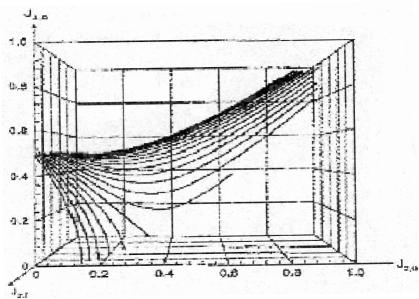
Figure 20: The Renormalization flow diagram for the model with finite range interactions according to [103]. The initial values are $J_{x,0}=0,J_{\perp,0}=0.5$, and $J_{x,l}$ varies from 0 to 1 in increments of 0.05. When $J_{z,l}$ becomes large enough (i.e. when $V$ is large enough) the flow veers from the usual Kondo fixed point to a zero hybridization ($J_{\perp,0}=0$) singular Fermi liquid.

3.7 A model for Mixed-Valence Impurity

We next consider a slightly more realistic model [190, 225, 229]

$${\mathcal{H}}=\sum_{k,\sigma,l}\epsilon_{kl}c^{\dagger}_{k\sigma l}c_{k\sigma l}+\epsilon_{d}n_{d,\uparrow}n_{d,\downarrow}+t\sum_{\sigma}\left(d_{\sigma}^{\dagger}c_{k\sigma 0}+h.c.\right)$$

$$+\sum_{k,k^{\prime},l}V_{kk^{\prime}l}\left(n_{d}-\frac{1}{2}\right)\left[\sum_{\sigma}c_{k\sigma l}^{\dagger}c_{k^{\prime}\sigma l}-1\right]~{}.$$ (67)

In this model both spin and charge may be altered on the impurity site. This enhanced number of degrees of freedom implies that the states need to be specified by more quantum numbers. This also allows, a priori, for higher degeneracy. In the following $N$ screening channels, all of equal strength $V$, will be assumed. In the $U\rightarrow\infty$ limit the spectrum of the impurity site may be diagonalized. The two lowest states are

$$\eta^{\dagger}\ 0\rangle = |0,1\rangle,~{}~{}\mbox{with energy}~{}E_{\eta}=-\frac{V\sqrt{N}}{4}-\frac{\epsilon_{d}}{2},$$

$$\zeta_{\sigma}^{\dagger}|0\rangle = |\sigma,0\rangle,~{}~{}\mbox{with energy}~{}E_{\zeta}=-\left[\left(\frac{\epsilon_{d}}{2}-\frac{V\sqrt{N}}{4}\right)^{2}+t^{2}\right]^{1/2},$$ (68)

where in the bras, the first entry is the charge and spin of the impurity spin and the second one is the compensating charge in the screening channels. Other states are elevated by energies ${\mathcal{O}}(V/\sqrt{N})$. The states satisfy the Friedel screening sum rule by having a small phase shift $\frac{\pi}{2N}$ in each of the $N$ channels. The parameter $V$ can be tuned to produce a degeneracy between the two states ($E_{\eta}=E_{\zeta}$) — the mixed valence condition. The enhanced degeneracy produces Singular Fermi-liquid like behavior. A perturbative calculation for small $\omega$ yields a self-energy

$$\Sigma\sim[\omega\ln\omega+i\omega sgn(\omega)]+O[(\omega\ln\omega)^{2}]~{}.$$ (69)

As a speculative note we remark that this physics might be of relevance to quantum dot problems. Quantum dots are usually described in terms of the Anderson model. However, there are certainly other angular momentum channels whereby the local charge on the dot and the external environment can interact. As the external potential in the leads is varied one is forced to pass through a potential in which this mixed valence condition must be satisfied. At this potential the aforementioned singular behavior should be observed.

3.8 Multi-channel Kondo problem

Blandin and Nozières [185] invented the multichannel Kondo problem and gave convincing arguments for a local singular Fermi-liquid behavior of it. Since then it has been solved by a multitude of sophisticated methods. For an overview of these and of applications of the multichannel Kondo problem, we refer to [212].

The multichannel Kondo problem is the generalization of the Kondo problem to the case in which the impurity spin has arbitrary spin $S$ and is coupled to $n$ “channels” of conduction electrons. The Hamiltonian is

$${\mathcal{H}}_{mcK}=t\sum_{\ell=1}^{n}\sum_{i<j}c^{(\ell)\dagger}_{i\alpha}c^{(\ell)}_{j\alpha}+J{\bf S}\cdot c^{(\ell)\dagger}_{0}{\bf\sigma}c_{0}^{(\ell)}~{}.$$ (70)

Here $\ell$ is the channel index. Degeneracy, the key to SFL behavior, is enforced through equal antiferromagnetic coupling $J>0$ for all the channels. When the couplings to the various channels are not all the same, at low enough temperatures a crossover to local Fermi-liquid behavior in the channel with the largest $J_{\ell}$ always occurs [7]. This crossover temperature is in general quite large compared to $T_{K}$ because channel asymmetry is a relevant perturbation about the symmetric fixed point. Therefore in comparing this theory with SFL behavior in experiments, one should ensure that one is above the crossover temperature.

The simple Kondo problem is the case $2S=1=n$. In this case at low temperatures a singlet state is formed of the impurity state and the conduction electron electrons in the appropriate channel. In the general multi-channel case in which $2S=n$, the physics is essentially the same, since there are exactly the right number of conduction electron channels to compensate the impurity spin at low temperatures. Thus, at low temperatures an effective spin 0 state is formed again, and the properties of the compensated Kondo problem $2S=n$ at finite temperature is that of crossover from a weakly interacting problem above the Kondo temperature $T_{K}$ to a strongly interacting problem below $T_{K}$.

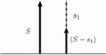
Figure 21: In a multichannel problem, a (Hund’s rule coupled) spin $S$ is compensated by total spin $S_{1}$ ($=n/2$) in $n$ different conduction electron channels leaving a net uncompensated spin as shown, or exact compensation or over-compensation when special properties may arise as discussed in the text.

The physics of the underscreened Kondo problem $2S>n$ is different. In this case, there are not enough conduction electron spins to compensate the impurity spin. As a result, when the temperature is lowered and the effective coupling increases, only a partial compensation of the impurity spin occurs by conduction electrons with spin opposite to it. As depicted in Fig. 21, a net spin in the same direction as the impurity spin then remains at the impurity site. Since the conduction electrons with their spin in the same directions as the impurity spin can then still make virtual excitations by hopping on that site while the site is completely blocked for conduction electrons with opposite spin, a net ferromagnetic coupling remains between the remaining effective spin and the conduction electrons. As a result, the low temperature physics of the underscreened Kondo problem is that of the ordinary ferromagnetic Kondo problem. To be more precise, the approach to the fixed point is analogous to that in the ferromagnetic Kondo problem along the boundary $J_{z}=-J_{\pm}$, because the impurity must decouple (become pseudo-classical) at the fixed point.

In the overscreened Kondo problem $2S<n$, there are more channels than necessary to compensate the impurity spin. At low temperatures, all $n$ channels tend to compensate the impurity spin due to the Kondo effect. Channel democracy now causes an interesting problem. As the effective interaction $J$ scales to stronger values, a local effective spin with direction opposite to the impurity spin results. This effective spin must have an effective antiferromagnetic interaction with the conduction electrons, since now the virtual excitations of conduction electrons with spins opposite to the effective local spin lower their energy. This then gives a new Kondo problem with a new effective interaction, and so on. Of course, in reality one does not get a succession of antiferromagnetic Kondo problems — the net effect is that a new stable finite-$J$ fixed point appears. As sketched in Fig. 22, the renormalized effective interaction flows to this fixed point both from the strong-coupling as well as from the weak-coupling side. One can understand this intuitively from the above picture: if one starts with a large initial value of $J$, then in the next order of perturbation theory about it, the interaction is smaller, since in perturbation theory the effective interaction due to virtual excitations decreases with increasing $J$. This means that $J$ scales to smaller values. Likewise, if we start from small $J$, then initially $J$ increases due to the Kondo scaling, but once $J$ becomes sufficiently large, the first effect which tends to decrease $J$ become more and more important. The finite-$J$ fixed point leads to nontrivial exponents for the low-temperature behavior of quantities like the specific heat,

$${{C_{v}}\over{T}}\propto\left({{T}\over{T_{K}}}\right)^{{n-2}\over{n+2}}~{}.$$ (71)

For $n=2$, the power law behavior on the right hand side is replaced by a $\ln T$ term.

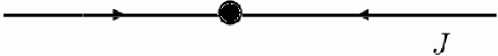
Figure 22: Flow diagram for the degenerate over-screened Kondo problem exhibiting a critical point.

Another way of thinking about the problem is in the spirit of Wilson’s renormalization group: Consider the problem of two channels interacting with a $S=1/2$ impurity. The conduction states can be expressed as linear combinations of concentric orbitals of conduction electrons around the impurity. These successive orbitals peak further and further away from the impurity. Consider first the exchange coupling of the orbitals in each of the two channels peaking at the impurity site. Each of them has $S=1/2$. Only one linear combination of the two channels, call it red, can couple, while the other (blue) does not. So after the singlet with the impurity is formed, we are left with a $S=1/2$, color blue problem. We must now consider the interaction of this effective impurity with the next orbital and so on. It is obvious that to any order we will be left with a spin 1/2 problem in a color. Conformal field theory methods first showed that the ground state is left with $1/2\ln 2$ impurity. A nice application of the bosonization method [83] identifies the red and blue above as linear combinations of the fermions in the two channels so that one is purely real, the other purely imaginary. The emergence of new types of particles — the Majorana fermions in this case — often happens at Singular Fermi-liquids.

As a detailed calculation confirms [7], the $J_{1}=J_{2}$ fixed point is unstable, and the flow is like sketched in Fig. 24. This means that the $J_{1}=J_{2}$ fixed point is a Quantum Critical Point: in the $T-J_{1}/J_{2}$ phase diagram, there is a critical point at $T=0,J_{1}/J_{2}=1$. Moreover, it confirms that asymmetry in the couplings is a relevant perturbation, so that the SFL behavior is unstable to any introduction of differences between the couplings to the different channels. The crossover temperature $T_{\times}$ below which two-channel behavior is replaced by the approach to the Kondo fixed point is [7]

$$T_{\times}={\mathcal{O}}\left(T_{K}(\bar{J})\left[(J_{1}-J_{2})/\bar{J}\right]^{2}\right)~{},$$ (72)

where $\bar{J}=(J_{1}+J_{2})/2$.

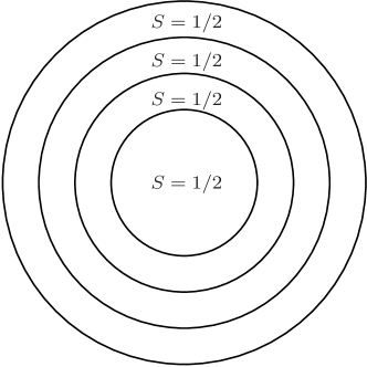
Figure 23: Effective shells in Energy space in Wilson’s method. The first shell integrates over a fraction $\lambda$ of the top of the band, the next shell $\lambda$ of the rest, and so on. In the two-channel $S=1/2$ problem, a $S=1/2$ effective impurity is left at every stage of interpretation.

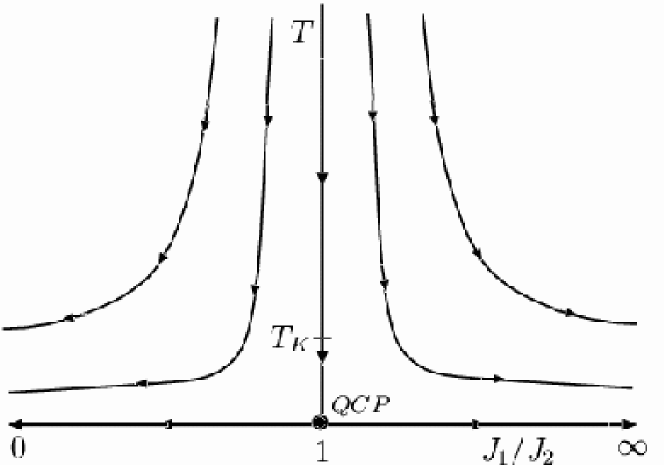
Figure 24: Flow in temperature-anisotropy plane for the two-channel Kondo problem with coupling constant $J_{1}$ and $J_{2}$.

The overscreened Kondo problem illustrates that the SFL behavior is associated with the occurrence of degeneracy: the critical point requires degeneracy of the two orthogonal channels.

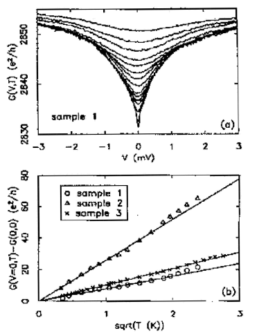
Figure 25: (a) Differential conductance $G(V,T)$ as a function of voltage $V$ in measurements on metal point contacts by Ralph et al. [205], for various temperatures ranging from 0.4 K (bottom curve) to 5.6 K (upper curve). Note the $\sqrt{V}$ type behavior developing as the temperature decreases. (b) The zero bias ($V=0$) conductance as a function of temperature for three different samples shows a $G(0,T)-G(0,0)\sim\sqrt{T}$ behavior. The scaling behavior as a function of voltage and temperature is consistent with two-channel Kondo behavior [205].

An interesting application of the two-channel Kondo problem is obtained by considering the spin label to play the role of the channel index, while the Kondo coupling is in the orbital angular momentum or crystal field states for impurities at symmetry sites in crystals [135, 69, 212]. Another possibility that has been considered is that of scattering of conduction electrons of two-level tunneling centers with different angular momentum states [287]. In this case, the tunneling model translates into a model with $x$ and $z$ coupling only, but this model flows towards a Kondo-type model with equal $x$ and $y$ spin coupling. For both types of proposed applications, one has to worry about the breaking of the symmetry, and about the question of how dilute the system has to be for a Kondo-type model to be realistic. Interesting results in the tunneling conductance of two metals through a narrow constriction, shown in Fig. 25 appear to bear resemblance to the properties expected of a degenerate two-channel Kondo effect [205, 70], but this interpretation is not undisputed [274, 206]. Applications to impurities in heavy fermions will be briefly discussed in section 6.4.

3.9 The Two-Kondo-Impurities Problem

In a metal with a finite concentration of magnetic impurities, an important question is what the (weak) interaction between the magnetic impurities does to the Kondo physics — that the effect might be substantial is already clear from the fact that the Kondo effect is seen in logarithmic corrections about the high-temperature local moment fixed point while the RKKY interaction between the moments mediated by the conduction electrons occur as a power law correction. Stated simply $T_{K}\sim{{1}\over{N(0)}}\exp(-{{1}\over{N(0)J}})$ while the RKKY interaction $I\sim J^{2}N(0)$. The existence of mixed-valence and heavy fermion metals makes this much more than an academic question. The question of the competition between these two effects, and in particular whether long range magnetic order can arise, was first posed by Varma [248] and by Doniach [76], who gave the obvious answer that RKKY interactions will be ineffective only when the Kondo temperature below which the local spin at each impurity is zero is much larger than the RKKY interaction I. Considering that $JN(0)$ is usually $\gg 1$, this is unlikely for $S=1/2$ problems, but for large $S$, as encountered typically in rare earths and actinides, it is possible in some cases. But the vast majority of rare earths and actinide compounds show magnetic order and no Heavy fermion magnetic behavior.

The two-Kondo-impurity problem serves as a first step to understanding some of the physics of heavy fermions. We will however only consider the $S=1/2$ problem and work with unrealistic $JN(0)$ so that the competition between the Kondo effect and RKKY is possible.

In this subsection we will summarize the results [128, 129, 8, 9, 229] for the two Kondo impurity problem; like the models we discussed above, this one also has a quantum critical point at which SFL behavior is found. However as for other impurity problems, an unrealistic symmetry must be assumed for a QCP and attendant SFL behavior.

The two-Kondo-impurity Hamiltonian is defined as

$${\mathcal{H}}=t\sum_{k,\sigma}c^{\dagger}_{k\sigma}c_{k\sigma}+J\;\left[{\bf S}_{1}\cdot{\bf\sigma}(r_{1})+{\bf S}_{2}\cdot{\bf\sigma}(r_{2})\right]~{}.$$ (73)

In this form, the problem has a symmetry with respect to the midpoint between the two impurity sites $r_{1}$ and $r_{2}$, and hence one can define even (e) and odd (o) parity states relative to this point. In the approximation that the $k$-dependence of the couplings is neglected [128] the two Kondo impurity Hamiltonian can then be transformed to

$${\mathcal{H}}={\mathcal{H}}_{non-interacting} + \sum_{kk^{\prime}}\left({\bf S}_{1}+{\bf S}_{2}\right)\cdot\left[J_{e}c^{\dagger}_{k^{\prime}e}{\bf\sigma}c_{ke}+J_{o}c^{\dagger}_{k^{\prime}o}{\bf\sigma}c_{ko}\right]$$ (74)

$$+ \sum_{kk^{\prime}}J_{m}\left({\bf S}_{1}-{\bf S}_{2}\right)\cdot\left[c^{\dagger}_{k^{\prime}e}{\bf\sigma}c_{ko}+c^{\dagger}_{k^{\prime}o}{\bf\sigma}c_{ke}\right]~{}.$$

The coupling between the spin and orbital channels generates an effective RKKY interaction

$${\mathcal{H}}_{RKKY}=I_{0}(J_{e},J_{o},J_{m})~{}{\bf S}_{1}\cdot{\bf S}_{2}$$ (75)

between the two impurity spins, with $I_{0}=2\ln 2(J_{e}^{2}+J_{o}^{2}-2J_{m}^{2})$ for $t=1$.

The main results of a numerical Wilson-type renormalization group treatment of this model are the following:

(i) For ferromagnetic coupling $I_{0}>0$ or for a small antiferromagnetic coupling $I_{0}>-2.24T_{K}$, where $T_{K}$ is the Kondo temperature of the single-impurity problem, one finds that there is a Kondo effect with

$$\langle{\bf S}_{1}\cdot{\bf S}_{2}\rangle\neq 0~{},$$ (76)

unless $I_{0}$ is very small, $|I_{0}/T_{K}|\ll 1$. Since for uncorrelated impurity spins $\langle{\bf S}_{1}\cdot{\bf S}_{2}\rangle=0$, (76) expresses that although in the RG language the RKKY interaction is an irrelevant perturbation, it is quite important in calculating physical properties due to large “corrections to scaling”. Another feature of the solution in this regime is the fact that the phase shift is $\pi/2$ in both channels. This means that at the fixed point the even-parity channel and the odd-parity channel have independent Kondo effects, each one having one electron pushed below the chemical potential in the Kondo resonance. As discussed below, this is due to particle-hole symmetry assumed in the model — without it, only the sum of the phase shifts in the two-channels is fixed.

(ii) There is no Kondo effect for $I_{0}<-2.24~{}T_{K}$. In this case, the coupling between the impurities is so strong that the impurities form a singlet among themselves and decouple from the conduction electrons. There is no phase shift at the fixed point. Also, in this case the total spin $S_{tot}=0$, but the impurity spins become only singlet like, $\langle{\bf S}_{1}\cdot{\bf S}_{2}\rangle\approx-3/4$ for very strong coupling, $I_{0}\ll-2.24~{}T_{K}$. So again there are important “corrections to scaling”.

(iii) The point $I_{0}=-2.24~{}T_{K}$ is a true critical point, at which the staggered susceptibility $\langle({\bf S}_{1}-{\bf S}_{2})^{2}\rangle/T$ diverges. Moreover, at this point the specific heat has a logarithmic correction to the linear $T$ dependence, $C_{v}\sim T\ln T$, while the impurity spin correlation function $\langle{\bf S}_{1}\cdot{\bf S}_{2}\rangle$ becomes equal to $-1/4$ at this value.

Although the approximate Hamiltonian (74) has a true quantum critical point with associated SFL behavior, we stress that the analysis shows that this critical point is destroyed by any $c^{\dagger}_{ke}c_{ko}$ coupling. A coupling of this type is not particle-hole symmetric; since the approximate Hamiltonian (74) is particle-hole symmetric, these terms are not generated under the renormalization group flow for (74). The physical two-Kondo-impurity problem (73), on the other hand, is not particle-hole symmetric. Therefore, the physical two Kondo impurity problem does not have a true quantum critical point — in other words, when the two-Kondo-impurity Hamiltonian (73) is approximated by (74) by ignoring $k$-independent interactions, relevant terms which destroy the quantum critical point of the latter Hamiltonian are also dropped. This has been verified in explicit analysis keeping the symmetry breaking terms [229].

An illuminating way to understand the result for the two-impurity Kondo problem, is to note that the Hamiltonian can be written in the following form:

$${\mathcal{H}}=\left[\hskip 5.69054pt\begin{array}[]{cc}\left[\begin{array}[]{cc}{\mathcal{H}}^{even}_{S=0}&0\\ 0&{\mathcal{H}}^{odd}_{S=0}\end{array}\right]&\left[\begin{array}[]{cc}0&{\mathcal{H}}_{mix}\\ {\mathcal{H}}_{mix}&0\end{array}\right]\\ \\ \left[\begin{array}[]{cc}0&{\mathcal{H}}_{mix}\\ {\mathcal{H}}_{mix}&0\end{array}\right]&\left[\begin{array}[]{cc}{\mathcal{H}}^{even}_{S=1}&0\\ 0&{\mathcal{H}}^{odd}_{S=1}\end{array}\right]\end{array}\hskip 5.69054pt\right]~{},$$ (77)

where ${\bf S}={\bf S}_{1}+{\bf S}_{2}$ is the total impurity spin.

In this representation, the Hamiltonian ${\mathcal{H}}_{mix}$ couples the $S=0$ and $S=1$ state, and the following interpretation naturally emerges: for large antiferromagnetic values of $I_{0}$, ${\mathcal{H}}_{S=0}$ is lower in energy than ${\mathcal{H}}_{S=1}$, while for large ferromagnetic coupling $I_{0}$, the converse is true. The two-Kondo impurity coupling can thus be viewed as one in which by changing $I_{0}$, we can tune the relative importance of the upper left block and the lower right block of the Hamiltonian. In general, the two types of states are mixed by ${\mathcal{H}}_{mix}$, but at the fixed point ${\mathcal{H}}^{*}_{mix}\rightarrow 0$. This implies that there is a critical value of $I_{0}/T_{K}$ where the $S=0$ and $S=1$ states are degenerate, and where SFL behavior occurs. At this critical value, the impurity spin is a linear combination of a singlet and triplet state with $\langle{\bf S}_{1}\cdot{\bf S}_{2}\rangle=-1/4$ (i.e. a value in between the singlet value -3/4 and the triplet value 1/4) and the singular low-energy fluctuations give rise to the anomalous specific heat behavior.

Within this scenario, the fact that the susceptibility $\chi$ is divergent at the critical point signals that a term ${\bf H}\cdot({\bf S}_{1}-{\bf S}_{2})$ lifts the spin degeneracy. Moreover, the leading irrelevant operators about the fixed point are all divergent at the critical point — of course, this just reflects the breakdown of the Fermi-liquid description.

The reason for ${\mathcal{H}}_{mix}\rightarrow 0$ is as follows. It arises from the last term in (74) which is not particle-hole symmetric because under even-odd interchange both the spin term and the fermion electron terms change sign. At the Kondo fixed point, the leading operators must all be biquadratic in fermions. An ${\mathcal{H}}_{mix}$ in that case would be of the form $c^{\dagger}_{k\sigma e}c_{k^{\prime}\sigma o}$ and and such a term by itself would break particle hole symmetry.

In the two-Kondo impurity problem, one encounters again the essentials of degeneracy for quantum critical points and the need for (unphysical) constraints to preserve the singularity. Once again new types of quantum numbers can be invoked in the excitations about the QCP.

From the point of view of understanding actual phenomena for problems with a moderate concentration of impurities or in reference to heavy fermion compounds, the importance of the solution to the two-Kondo impurity problem is the large correction to scaling found in the Wilson-type solution away from the special symmetries required to have a QCP. These survive quite generally and must be taken into account in constructing low-energy effective Hamiltonians in physical situations.

4 SFL behavior for interacting fermions in one dimension

A variety of elegant mathematical techniques, including exact solutions in certain nontrivial limits, have been employed to analyze the problem of interacting electrons in one dimension. We discuss the essential features of these models here and their SFL properties. We also discuss whether the methods and the results can be extended to higher dimensions.

Some cases where the models solved are experimentally realized include the edge states of Quantum Hall liquids and quasi-one dimensional organic and inorganic compounds [81, 82]. In the latter case, the asymptotic low energy properties are, however, unlikely to be those of the 1D models because of the inevitable coupling to the other dimensions which proves to be a relevant perturbation. Nonetheless, data on carbon nanotubes [73] discussed in section 4.11 show clear evidence of one-dimensional interacting electron physics. Several one-dimensional spin chains problems can also be transformed into problems of one-dimensional fermions [210].

Our aim in this chapter is to highlight the physics leading to the Singular Fermi Liquid behavior and to present the most important results obtained. Detailed reviews of the technical steps in the various solutions as well as numerical calculations may be found in [109, 231]. As pointed out already in section 2.6, logarithmic singularities appear in the second order perturbative calculation of the vertices in the 1D problem (both in the particle-hole and particle-particle channels). We present the $T=0$ phase diagram as obtained by summing those singularities by perturbative RG. This will be followed by a discussion of the results of the exact solution of the Tomonaga-Luttinger and the more general model for special values of the coupling constants (along the so called “Luther-Emery” line [155]).

One special feature of 1D physics is that the low energy excitations can be described by either fermions or bosons. The bosonic description of the Tomonaga-Luttinger model is especially attractive and will be presented below.

A distinctive feature of one dimensional physics is that single-particle as well as multiple-particle correlation functions are expressible in terms of independent charge and spin excitations, which, in general, propagate with different velocities This feature has been shown to arise due to extra conservation laws in one dimensions [50, 167]. As we shall discuss, an extension of charge-spin separation to higher dimensions is unlikely because there are no such conservation laws.

The one dimensional singularities may be also seen as a manifestation of the orthogonality catastrophe [20] that we discussed in section 3.4. We shall see that this feature disappears in higher dimension due to the effects of recoil.

4.1 The One Dimensional Electron Gas

The Hamiltonian describing the low energy dynamics reads

$${\mathcal{H}}={\mathcal{H}}_{0}+{\mathcal{H}}_{forward}+{\mathcal{H}}_{backward}+{\mathcal{H}}_{Umklapp}~{}.$$ (78)

In (78) ${\mathcal{H}}_{0}$ is the free electron Hamiltonian

$${\mathcal{H}}_{0}=\sum_{k}\epsilon_{k}c^{\dagger}_{k}c_{k}~{}.$$ (79)

In one dimension the particles move in two branches, either to the left or the right. Define the charge density operators $\rho_{r}$ and the spin density operators $S_{r}$ for the two branches, $r=\pm$,

$$\rho_{r}=\Sigma_{\sigma=\pm 1}\psi_{r,\sigma}^{\dagger}\psi_{r,\sigma}~{},~{}~{}~{}~{}~{}~{}S^{z}_{r}=\frac{1}{2}\Sigma_{\sigma,\sigma^{\prime}}\psi^{\dagger}_{r,\sigma}\tau^{z}_{\sigma,\sigma^{\prime}}\psi_{r,\sigma^{\prime}}~{},$$ (80)

where $\tau^{z}$ is a Pauli-matrix. The Fourier components of the particle density operators read

$$\rho_{r,\sigma}(q)=\sum_{k}c_{r,\sigma,k+q}^{\dagger}c_{r,\sigma,k}=\rho^{\dagger}_{r,\sigma}(-q)~{}.$$ (81)

These bilinears may be explicitly shown to obey Bose commutation relastions. If we linearize $\epsilon_{k}$ about the two Fermi-points, the energy of a particle-hole pair created by $\rho_{r,\sigma}(q)$,

$$\epsilon_{r,k+q}-\epsilon_{r,k}=rv_{F}q~{},$$ (82)

is independent of $k$ in one dimension (provided the band cutoff is taken to infinity). States created by $\rho_{r,\sigma}(q)$ are linear combinations of individual electron-hole excitations all of which have the same energy and are therefore eigenstates of ${\mathcal{H}}_{0}$. It follows that for $q>0$, $\rho_{r=+,\sigma}(q)$ [$\rho_{r=-,\sigma}(q)$] is a raising [lowering] operator. Consequently ${\mathcal{H}}_{0}$ may be expressed in terms of the density operators:

$${\mathcal{H}}_{0}=\frac{2\pi v_{F}}{L}\sum_{r=\pm}\sum_{q>0}\rho_{r,\sigma}(rq)\rho_{r,\sigma}(-rq)~{}.$$ (83)

Upon separating the densities on a given branch into charge and spin pieces,

$$\rho_{r\sigma}(x)=\frac{1}{2}[\rho_{r}(x)+\sigma S_{r}^{z}(x)]~{},$$ (84)

the free Hamiltonian may be expressed as a sum in the spin and charge degrees of freedom:

$${\mathcal{H}}_{0}=\sum_{r}{\cal{H}}_{0}[\rho_{r}]+\sum_{r}{\cal{H}}_{0}[S_{r}^{z}].$$ (85)

It follows that in the noninteracting problem spin and charge have identical dynamics and propagate in unison. Once interactions are introduced, the electron will “fractionalize” and spin and charge dynamics will, in general, differ.

We now discuss the various interaction terms in the Hamiltonian. The piece describing the forward scattering events $(k_{F},\sigma;-k_{F},\sigma^{\prime})$ $\rightarrow$ $(k_{F},\sigma;-k_{F},\sigma^{\prime})$ and $(k_{F},\sigma;k_{F},\sigma^{\prime})$ $\rightarrow(k_{F},\sigma;k_{F},\sigma^{\prime})$ reads

$${\mathcal{H}}_{forward}={\mathcal{H}}_{2}+{\mathcal{H}}_{4}~{},$$ (86)

with

$${\mathcal{H}}_{2} = \frac{1}{L}\sum_{q}\sum_{\sigma\sigma^{\prime}}g_{2}^{\sigma\sigma^{\prime}}\rho_{+,\sigma}(q)\rho_{-,\sigma^{\prime}}(-q)~{},$$ (87)

$$H_{4} = \frac{1}{2L}\sum_{q}\sum_{\sigma\sigma^{\prime}}g_{4}^{\sigma\sigma^{\prime}}[\rho_{+,\sigma}(q)\rho_{+,\sigma^{\prime}}(-q)+\rho_{-,\sigma}(q)\rho_{-,\sigma^{\prime}}(-q)]~{}.$$ (88)

The operators $\rho_{r,\sigma}$ involve a creation and annihilation operator on the same branch. We also define operators $\rho^{r}_{\sigma}$ which involve operators on opposite branches,

$$\rho_{\sigma}^{r}=\sum_{k}c^{\dagger}_{r,\sigma,k}c_{-r,\sigma,k+q}~{}.$$ (89)

In terms of these the Hamiltonian describing backscattering interactions (the scattering event $(+k_{F},\sigma;-k_{F},\sigma^{\prime})\rightarrow(-k_{F},\sigma;k_{F},\sigma^{\prime})$ and its reverse) becomes

$${\mathcal{H}}_{backwards}={\mathcal{H}}_{1}=g_{1}\sum_{q}\sum_{\sigma\sigma^{\prime}}g_{1}^{\sigma\sigma^{\prime}}\rho_{\sigma}^{+}(q)\rho_{\sigma^{\prime}}^{-}(-q)~{}.$$ (90)

and the Umklapp term reads

$${\mathcal{H}}_{3}=\frac{1}{2L}\sum_{q}\sum_{\sigma\sigma^{\prime}}g_{3}^{\sigma\sigma^{\prime}}[\rho_{\sigma}^{+}(q)\rho_{\sigma^{\prime}}^{+}(-q)+\rho^{-}_{\sigma}(q)\rho^{-}_{\sigma^{\prime}}(-q)]~{}.$$ (91)

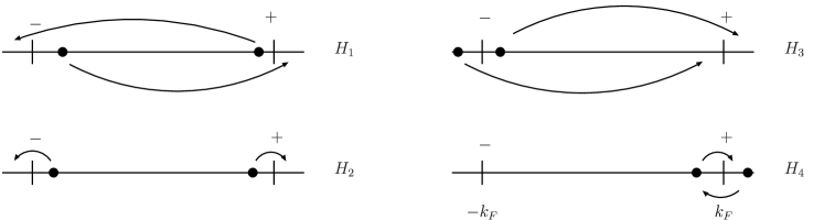
Figure 26: Pictorial representation of the low-energy interaction terms in the one-dimensional problem. After [169]. The “+” and “-” points are a shorthand for the two Fermi points $k=k_{F}$ and $(-k_{F})$ respectively.

In all these expressions, the coupling constants may be spin dependent:

$$g_{i}^{\sigma\sigma^{\prime}}=g_{i||}\delta_{\sigma\sigma^{\prime}}+g_{i\perp}\delta_{\sigma-\sigma^{\prime}}~{}.$$ (92)

As the terms $H_{1||}$ and $H_{2||}$ describe the same process we may set $g_{1||}=0$ with no loss of generality. Umklapp processes are important only when $4k_{F}$ is a reciprocal lattice vector so that all scattering particles may be near the Fermi points. If the one dimensional electronic system is sufficiently incommensurate then these processes may be neglected.

The condition for spin rotation invariance $[{\mathcal{H}},\vec{S}]=0$ reads

$$g_{2\perp}-g_{1\perp}=g_{2||}-g_{1||}~{}.$$ (93)

A guide to the behavior of the Hamiltonian (78) is obtained from the perturbative Renormalization Group flow equations. In one dimension, there are no truly ordered phases, but at $T=0$ there is algebraic long range order. One may thus determine a “phase diagram” according to which susceptibilities diverge as $T\rightarrow 0$: the one associated with singlet superconductivity ($SS$), triplet superconductivity ($TS$), charge density wave ($CDW$) state at $2k_{F}$, and spin density wave ($SDW$) state at $2k_{F}$. The expressions for these susceptibilities are given in Eq. (111) below, and the resulting “phase diagram” is shown in Fig. 27.

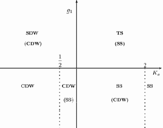
Figure 27: Phase diagram for one-dimensional interacting fermions in the $(K_{c},g_{1})$ plane with $g_{1||}=0$ in Eqn. (92) and $K_{c}$ given by Eq.102  . $SDW$ and $(CDW)$ in the upper left quadrant indicates that both the spin density wave susceptibility and the charge density wave susceptibility diverge as $T\to 0$, but that the spin density wave susceptibility diverges a factor $\ln^{2}T$ faster than the charge density wave susceptibility — see Eq. (111). Other sectors are labeled accordingly. From [218].

4.2 The Tomonaga-Luttinger Model

With forward scattering alone in (78) and after linearizing the kinetic energy we obtain the Tomonaga-Luttinger (T-L)model. In terms of fermion field operators $\psi_{r,\sigma}(x)$ and $\psi_{r,\sigma}^{\dagger}(x)$, and density and spin operators $\rho_{r}(x)$ and $S_{r}^{z}(x)$ in real space, the T-L model is

$${\mathcal{H}}^{T-L} =\int dx~{}\left[-v_{F}\sum_{r,\sigma=\pm}r\psi_{r,\sigma}^{\dagger}i\partial_{x}\psi_{r,\sigma}+\frac{1}{2}\sum_{r=\pm}g_{2,c}\rho_{r}(x)\rho_{-r}(x)\right]$$ (94)

$$+\left.\sum_{r=\pm}g_{4,c}\rho_{r}(x)\rho_{r}(x)+2\sum_{r=\pm}g_{2,s}S_{r}^{z}(x)S_{-r}^{z}(x)+g_{4,s}S_{r}^{z}(x)S_{r}^{z}(x)\right].$$

where

$$g_{i}^{c}=\frac{g_{i||}+g_{i\perp}}{2}~{},~{}~{}~{}~{}~{}~{}g_{i}^{s}=\frac{g_{i||}-g_{i\perp}}{2}~{}.$$ (95)

Note that the $g_{2,s}$ term is the only term which break $SU(2)$ spin symmetry. The T-L model is exactly solvable. After all, as previously noted, the (Dirac-like) kinetic energy Hamiltonian ${\mathcal{H}}_{0}$ is also quadratic in the density operators. So the Hamiltonian is readily diagonalized by a Bogoliubov transformation whereupon the Hamiltonian becomes a sum of two independent (harmonic) parts describing noninteracting charge and spin density waves: the charge and spin density waves are the collective eigenmodes of the system.

The simplest way to describe the TL model and to explicitly track down these collective modes is via the bosonization of the electronic degrees of freedom. The reader should be warned that many different conventions abound in the literature. The bosonic representation of the fermionic fields proceeds by writing [109, 180, 210]

$$\psi_{r,\sigma}(x)=\lim_{a\rightarrow 0}\frac{\exp[ir(k_{F}x+\Phi_{r\sigma}(x))]}{\sqrt{2\pi a}}F_{r\sigma}~{},$$ (96)

where $a$ is a short distance regulator. $\Phi_{r\sigma}(x)$ satisfies

$$[\Phi_{r\sigma}(x),\Phi^{\dagger}_{r^{\prime},\sigma^{\prime}}(x^{\prime})]=-i\pi\delta_{r,r^{\prime}}\delta_{\sigma,\sigma^{\prime}}\mbox{sign}(x-x^{\prime})~{}.$$ (97)

The “Klein factors” $F_{r\sigma}$ are chosen such that the proper fermionic anticommutation relations are reproduced. The exponential envelope $\exp[i\Phi_{r\sigma}(x)]$ represents the slow bosonic collective degrees of freedom which dress the rapidly oscillating part $F_{r\sigma}\exp[ik_{F}x]$ describing the energetic particle excitations near the Fermi points.

$\Phi$ may be written in terms of the bosonic fields $\phi_{c,s}$ and their conjugate momenta $\partial_{x}\theta_{c,s}$

$$\Phi_{r,\sigma}=\sqrt{\pi/2}[(\theta_{c}-r\phi_{c})+\sigma(\theta_{s}-r\phi_{s})]~{}.$$ (98)

In terms of the new variables, the charge and spin densities read

$$\rho(x)=\sum_{r}\rho_{r}(x)=\sqrt{\frac{2}{\pi}}\partial_{x}\phi_{c}~{},~{}~{}~{}~{}~{}~{}S^{z}(x)=\sum_{r}S_{r}^{z}(x)=\sqrt{\frac{1}{2\pi}}\partial_{x}\phi_{s}~{}.$$ (99)

In the $(\theta_{c,s},\phi_{c,s})$ representation the Tomonaga-Luttinger Hamiltonian becomes a sum of two decoupled oscillators describing the gapless charge and spin density wave eigenmodes

$${\mathcal{H}}^{T-L}=\int dx~{}\sum_{\nu=c,s}\frac{v_{\nu}}{2}\left[K_{\nu}(\partial_{x}\theta_{\nu})^{2}+\frac{(\partial_{x}\phi_{\nu})^{2}}{K_{\nu}}\right]\equiv{\cal{H}}_{s}^{T-L}+{\cal{H}}_{c}^{T-L}.$$ (100)

The velocities of the collective charge and spin modes are easily read of by analogy to a harmonic string:

$$v_{c,s}=\sqrt{(v_{F}+\frac{g_{4}^{c,s}}{\pi})^{2}-(\frac{g_{2}^{c,s}}{\pi})^{2}}~{}.$$ (101)

Likewise, the moduli determining the power-law decay of the correlations are

$$K_{c,s}=\sqrt{\frac{\pi v_{F}+g_{4}^{c,s}-g_{2}^{c,s}}{\pi v_{F}+g_{4}^{c,s}+g_{2}^{c,s}}}~{}.$$ (102)

In section 4.7 we shall show how the above expressions for the spin and charge density wave velocities follow simply from the conservation of left and right moving particles in the T-L model.

As previously noted, the charge and spin velocities are degenerate in the noninteracting model. When interactions are introduced, the charge and spin velocities ($v_{c}$ and $v_{s}$) as well as the energy to create spin and charge excitations ($(v_{s}/K_{s}$ and $v_{c}/K_{c}$ respectively) become different. The charge constant $K_{c}$ is less than 1 for repulsive interactions, which elevates the energy of the charge excitations, while $K_{c}$ is greater than 1 for attractive interactions.

4.3 One-particle Spectral functions

The zero temperature spectral functions of the T-L model are

$$A(k,\omega)\approx(\omega-v_{c}(k-k_{F}))^{2\gamma_{c}-1/2}|\omega-v_{c}(k-k_{F})|^{\gamma_{c}-1/2}~{}~{}~{}(v_{c}>v_{s})$$

$$A(k,\omega)\approx(\omega-v_{s}(k-k_{F}))^{\gamma_{c}-1/2}|\omega-v_{s}(k-k_{F})|^{2\gamma_{c}-1/2}~{}~{}~{}(v_{c}<v_{s}).$$ (103)

These spectral functions are sketched in Fig. 28 for the case $g_{2}=0$ and in Fig. 29 for the general case. Notice that the quasiparticle pole in $A(k,\omega)$ in a Landau Fermi-liquid is smeared out to produce a branch cut extending from the spin mode excitation energy to the charge mode excitation energy. These branch cuts split into two in an applied magnetic field, see Fig. 30. These results are exact for small $\omega$ and small $|k-k_{F}|$. Another manifestation of the SFL behavior is the behavior of the momentum distribution function

$$n_{k}\sim n_{k_{F}}-const\times\mbox{sign}(k-k_{F})|k-k_{F}|^{2\gamma_{c}}~{},$$ (104)

where

$$\gamma_{c,s}=\frac{1}{8}\left(K_{c,s}+K_{c,s}^{-1}-2\right)~{}.$$ (105)

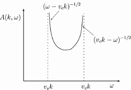
Figure 28: The zero temperature spectral function $A(k,\omega)=\mbox{Im}\{G_{r=+1}^{<}(k,\omega)\}$ as a function of $\omega$ for the case ($g_{2}=0,~{}g_{4}\neq 0$) — the “one-branch Luttinger liquid” in which the spin and charge velocities differ but for which the the correlation exponents keep their canonical $K_{c}=1$ according to (102). In the figure $v_{c}>v_{s}$ and $k>0$ are assumed. Note the inverse square root singularities. This is a consequence of $K_{c}=1$ which makes $\gamma_{c}=0$. After Voit [262].

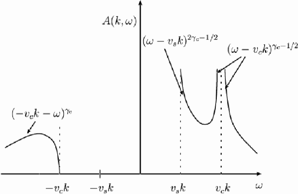
Figure 29: The generic $(g_{2}\neq 0,g_{4}\neq 0$) zero temperature spectral function. Note the broader range of non-trivial singularities near $v_{s}k$ and $\pm v_{c}k$. Here both the effect of spin-charge velocity difference and the emergence of non-trivial exponents is visible. After Voit [262]

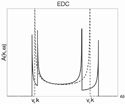
Figure 30: The energy distribution curve (the spectrum $A(k,\omega)$ at fixed $k$) as a function of $\omega$ in the presence of a magnetic field. The dashed line is the zero-field result of Fig. 28. The magnitude of the Zeeman splitting is enhanced with respect to $(v_{c}-v_{s})k$ for clarity. From Rabello and Si [204].

In contrast to a Fermi liquid, the expression for $n_{k}$ does not exhibit a step-like discontinuity at the Fermi points. Note that the exponent $2\gamma_{c}$ is non-universal (as usual, an outcome of a line of critical points).

The single particle density of states

$$N(\omega)\approx|\omega|^{2\gamma_{c}}~{},$$ (106)

vanishes at the Fermi surface.

4.4 Thermodynamics

The contributions of the independent charge and spin modes appears independently in most physical quantities.

The specific heat coefficient is found to be

$$\gamma/\gamma_{0}=\frac{v_{F}}{2}\left(\frac{1}{v_{c}}+\frac{1}{v_{s}}\right).$$ (107)

where $\gamma=\gamma_{0}$ for the non-interacting system.

The spin susceptibility and the compressibility are readily computed

$$\chi_{0}=v_{F}/v_{s}~{},~{}~{}~{}~{}~{}~{}~{}\kappa/\kappa_{0}=v_{F}K_{c}/v_{c}$$ (108)

where $\chi_{0}$ and $\kappa_{0}$ are the susceptibility and compressibility of the noninteracting gas. The Wilson ratio, already encountered in our discussion of the Kondo problem in section 3.2,

$$R_{W}=\frac{\chi/\chi_{0}}{\gamma/\gamma_{0}}=\frac{2v_{c}}{v_{c}+v_{s}}~{},$$ (109)

deviates from its Fermi Liquid value of unity by an amount dependent on the relative separation between the spin and charge velocities.

4.5 Correlation Functions

Since the Hamiltonian is separable in charge and spin and as $\psi$ is a product of independent charge and spin degree of freedom all real space correlation functions are products of independent charge and spin factors. We will only focus on the most important correlation functions in the illustrative examples below, and refer for a summary of the various exact expressions to [188].

The most important feature of the large distance behavior of the charge and spin correlators is their algebraic decay at zero temperature:

$$\langle\rho(x)\rho(x^{\prime})\rangle \simeq \frac{K_{c}}{(\pi(x-x^{\prime}))^{2}}+B_{1,c}\frac{\cos(2k_{F}(x-x^{\prime}))}{|x-x^{\prime}|^{1+K_{c}}}\ln^{-3/2}|x-x^{\prime}|$$ (110)

$$\hskip 56.9055ptB_{2,c}\frac{\cos(4k_{F}(x-x^{\prime}))}{|x-x^{\prime}|^{4K_{c}}}+...$$

$$\langle\vec{S}(x)\cdot\vec{S}(x^{\prime})\rangle \simeq \frac{1}{(\pi(x-x^{\prime}))^{2}}+B_{1,s}\frac{\cos(2k_{F}(x-x^{\prime}))}{|x-x^{\prime}|^{1+K_{c}}}\ln^{1/2}|x-x^{\prime}|+...$$

at asymptotically long distances and $K_{s}=1$. For not too repulsive interactions, so that $K_{c}<1$, the $2k_{F}$ fluctuations are dominant. We have previously seen that such a CDW/SDW instability may arise due to the special $2k_{F}$ nesting wavevector in one dimension. The $4k_{F}$ modulations are due to Umklapp scattering. The amplitudes $\{B_{i,c}\}$ and $\{B_{i,s}\}$ are non-universal while the exponents are determined by the stiffness of the free charge and spin fields.

While the above expressions are for $K_{s}=1$, in the general case $K_{s}\neq 1$ the spin correlator decays asymptotically with the exponent $(K_{s}+K_{c})$.

At nonzero temperatures, it is found that the Fourier transforms of these correlation functions scale as

$$\chi_{CDW} \approx T^{K_{c}-1}|\ln T|^{-3/2}~{},~{}~{}~{}~{}~{}\chi_{SDW}\approx T^{K_{c}-1}|\ln T|^{1/2}~{},$$

$$\chi_{SS} \approx T^{K_{c}-1}|\ln T|^{-3/2}~{},~{}~{}~{}~{}~{}~{}~{}~{}\chi_{TS}\approx T^{K_{c}-1}|\ln T|^{1/2}~{}.$$ (111)

An example of the spectral density as a function at finite temperatures is shown in Fig. 31.

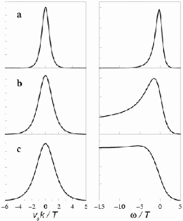
Figure 31: Left panel: Momentum distribution curves at $\omega=0$ (i.e., the spectrum at fixed $\omega=0$ as a function of $k$) for a spin rotationally invariant Tomonaga-Luttinger liquid, plotted as a function of $v_{s}k/T$. Right panels: Energy distribution curves at $k=0$ (the spectrum at fixed $k=0$) as a function of $\omega/T$. In both panels, $v_{c}/v_{s}=3$ and $\gamma_{c}=0$ in (a), $\gamma_{c}=0.25$ in (b), and $\gamma_{c}=0.5$ in (c). From Orgad [188].

The results above lead in principle to clear experimental signatures. $X$-rays, which couple to the charge density waves, should peak at low temperatures with intensities given by

$$I_{2k_{F}}\sim T^{K_{c}},~{}~{}~{}I_{4k_{F}}\sim T^{2K_{c}-1}~{}.$$ (112)

The NMR probe couples to the spin degrees of freedom and the theoretically computed nuclear relaxation time scales as

$$T_{1}\sim T^{-K_{c}}~{}.$$ (113)

4.6 The Luther-Emery Model

The Luther Emery model extends the Tomonaga-Luttinger Hamiltonian by including the backward scattering interactions parametrized by ${\mathcal{H}}_{1}$, which scatter from $(+k_{F},\sigma;-k_{F},\sigma^{\prime})$ to $(-k_{F},\sigma;k_{F},\sigma^{\prime})$ and vice versa. The Umklapp processes, important (at $T=0$) only when $4k_{F}$ is a reciprocal lattice, continue to be discarded.

The backward scattering term

$${\mathcal{H}}_{1}=\int dx~{}g_{1}\sum_{r=\pm 1}\psi_{r,\sigma=+1}^{\dagger}\psi_{-r,\sigma=-1}^{\dagger}\psi_{r,\sigma=-1}\psi_{-r,\sigma=1}$$ (114)

written in terms of the bosonic variables introduces a nontrivial sine-Gordon like interaction:

$${\cal{H}}_{s}=\int dx\frac{v_{s}}{2}\left[K_{s}(\partial_{x}\theta_{s})^{2}+\frac{(\partial_{x}\phi_{s})^{2}}{K_{s}}\right]+\frac{2g_{1}}{(2\pi a)^{2}}\cos(\sqrt{8\pi}\phi_{s})$$ (115)

with rescaled values of the spin and charge velocities and stiffness constants. When $g_{1}>0$ (repulsive interactions), $g_{1}$ is renormalized to zero in the long wavelength limit. Since along the RG flow trajectories $K_{s}-1\approx g_{1}/(\pi v_{s})$, this means that $K_{s}$ renormalizes to 1. The physics corresponding to this case is in the Tomonaga-Luttinger model that we just discussed.

When the backscattering interactions are attractive, $g_{1}<0$, spin excitations are no longer gapless, and a spin gap of magnitude

$$\Delta_{s}\sim\frac{v_{s}}{a}\left[\frac{g_{1}}{2\pi^{2}v_{s}}\right]^{1/(2-2K_{s})}$$ (116)

is dynamically generated. The attractive backscattering leads to the formation of bound particle-hole pairs which form a CDW. The spin correlation length is then finite,

$$\xi_{s}=\frac{v_{s}}{\Delta_{s}}~{}.$$ (117)

Gaps in the charge spectrum develop in the presence of Umklapp scattering. In the spin gapped phase the Hamiltonian can be conveniently expressed in terms of new refermionized spin fields $\Psi_{r}(x)$.

$$\Psi_{r}=F_{r}\exp[-i\sqrt{\pi/2}(\theta_{s}-2r\phi_{s})]~{}.$$ (118)

Luther and Emery observed that at the point $K_{s}=1/2$ the Hamiltonian in terms of these new spin fields becomes that of noninteracting free fermions having a mass gap $\Delta_{s}=g_{1}/(2\pi a)$.

$${\cal{H}}_{s}=\int dx\sum_{r=\pm 1}[-iv_{s}r\Psi_{r}^{\dagger}\partial_{x}\Psi_{r}+\Delta_{s}\Psi_{r}^{\dagger}\Psi_{-r}]~{},$$ (119)

leading to the spin excitation spectrum

$$E_{s}=\sqrt{\Delta_{s}^{2}+v_{s}^{2}(k-k_{F})^{2}}~{}.$$ (120)

4.7 Spin charge separation

As in many other physical problems, the availability of an exact solution to the one-dimensional electron gas problem is intimately linked to the existence of additional conservation laws or symmetries. One may attack the Luttinger Liquid problem by looking for its symmetries.

The $U(1)_{L}\otimes U(1)_{R}$ symmetry in the absence of Umklapp scattering may be exhibited by considering the effect of the separate left and right rotations by angles $\Gamma_{L,R}$ on the fermion variables:

$$\psi_{L\sigma}(x,t)\rightarrow e^{i\Gamma_{L}}\psi_{L\sigma}(x,t)~{},~{}~{}~{}~{}~{}~{}\psi_{R\sigma}(x,t)\rightarrow e^{i\Gamma_{R}}\psi_{R\sigma}(x,t)~{}.$$ (121)

All of the currents are trivially invariant under this transformation as the $\psi^{\dagger}$ fields transform with opposite phases. Physically this corresponds to the conservation of the number and net spin of left and right moving particles.

As discussed by Metzner and Di Castro [167], these separate conservation laws for the left and right moving charge and spin currents lead to Ward identities which enable the computation of the single particle correlation functions.

In the absence of Umklapp scattering, spin and charge are conserved about each individual Fermi point. The net total charge density $\rho\equiv\rho_{+}+\rho_{-}$ and charge density asymmetry $\tilde{\rho}\equiv\rho_{+}-\rho_{-}$ in the Tomonaga-Luttinger Hamiltonian satisfy the continuity equations

$$\partial_{\tau}\rho=[{\mathcal{H}},\rho]=-q{j}~{},~{}~{}~{}~{}~{}~{}\partial_{\tau}\tilde{\rho}=[{\mathcal{H}},\tilde{\rho}]=-q\tilde{j}~{},$$ (122)

where

$$j(q)=u_{c}[\rho_{+}-\rho_{-}]~{},~{}~{}~{}~{}~{}~{}\tilde{j}=\tilde{u}_{c}[\rho_{+}+\rho_{-}]~{},$$ (123)

and where the velocities are given by

$$u_{c}=v_{F}+\frac{g_{4}^{c}-g_{2}^{c}}{\pi}~{},~{}~{}~{}~{}~{}~{}\tilde{u}_{c}=v_{F}+\frac{g_{4}^{c}+g_{2}^{c}}{\pi}~{}.$$ (124)

These results follow straightforwardly from the form of ${\mathcal{H}}^{T-L}$ in combination with the fact that the only nonzero commutator is

$$[\rho_{r,\sigma}(q),\rho_{r^{\prime},\sigma^{\prime}}(-q^{\prime})]=\delta_{qq^{\prime}}\delta_{rr^{\prime}}\delta_{\sigma\sigma\prime}\left({{qL}\over{2\pi}}\right)~{}.$$ (125)

Let us illustrate simply how many of the results derived via bosonization may also be directly computed by employing these conservation laws. The existence of gapless charge modes is a direct consequence of the right-left charge conservation laws. The two first-order continuity equations given above lead to

$$[\partial_{\tau}^{2}+u_{c}\tilde{u}_{c}q^{2}]\rho=0~{},$$ (126)

from which we can read off a linear charge dispersion mode

$$\omega=v_{c}|q|$$ (127)

with velocity $v_{c}=\sqrt{u_{c}\tilde{u}_{c}}$, in agreement with the earlier result (101). Thus, collective charge excitations propagate with a velocity $v_{c}$. A similar relation may be found for the spin velocity $v_{s}$ which in general is different from $v_{c}$. This spin-charge separation also becomes clear from the explicit form of the expectation values of the charge and spin densities:

$$\langle 0|\psi_{r}(x_{0})\rho_{r}(x,t)\psi^{\dagger}_{r}(x_{0})|0\rangle = \delta(x-x_{0}-rv_{c}t)~{},$$

$$\langle 0|\psi_{r}(x_{0})S_{r}^{z}(x,t)\psi^{\dagger}_{r}(x_{0})|0\rangle = \delta(x-x_{0}-rv_{s}t)~{},$$ (128)

where $|0\rangle$ denotes the ground state.

The separate Right–Left conservation laws cease to hold if (back-scattering) impurities are present. Accordingly, as shown by Giamarchi and Schulz, [104] spin-charge separation then no longer holds.

4.8 Spin-charge Separation in more than one-dimension?

Spin-Charge separation in one dimension requires extra conservation laws. Can something analogous happen in more than one-dimension? No extra conservation laws are discernible in the generic Hamiltonians in two-dimension, although such Hamiltonians can doubtless be constructed. Are there conditions in which generic Hamiltonians become dynamically equivalent to such special Hamiltonians (because the unwelcome operators are ”irrelevant”). No definite answers to these questions are known. In section (5.2)and later in this section we shall briefly review some interesting attempts towards spin-charge separation in higher dimensions. First we present qualitative arguments pointing out the difficulty in this quest.

There is a simple caricature given by Schulz [218] for qualitatively visualizing charge-spin separation for a special one-dimensional case: the $U\rightarrow\infty$ Hubbard model. This model is characterized (at half-filling) by algebraic decay of Spin-Density correlations, which at short distances appear as almost antiferromagnetic alignments of spins. Let us track the motion of a hole introduced into an antiferromagnetically ordered chain. The hole is subject to only the lattice kinetic term which enables it to move by swapping with a nearby spin.

An initial configuration will be

$$...\Downarrow\Uparrow\Downarrow\Uparrow\Downarrow O\Downarrow\Uparrow\Downarrow\Uparrow\Downarrow...$$ (129)

After one move the configuration is

$$...\Downarrow\Uparrow\Downarrow\Uparrow O\Downarrow\Downarrow\Uparrow\Downarrow\Uparrow\Downarrow...$$ (130)

After two additional moves to the left the configuration reads

$$...\Downarrow\Uparrow O\Downarrow\Uparrow\Downarrow\Downarrow\Uparrow\Downarrow\Uparrow\Downarrow...$$ (131)

Thus the initial hole surrounded by two spins of the same polarization has broken into a charge excitation (“holon” or “chargon” — a hole surrounded by antiferromagnetically aligned spins) and a spin excitation (“spinon”) composed of two consecutive parallel spins in an antiferromagnetic environment. The statistics of the localized spinons and holons in this model must be such that their product is fermionic.

The feasibility of well defined spin and charge excitations hinges on the commuting nature of the right and left kinetic (hopping) operators $T_{Right},T_{Left}$ which are the inverse each other. Any general term of the form

$$(T_{Left})^{n_{1}^{Left}}(T_{Right})^{n_{1}^{Right}}(T_{Left})^{n_{2}^{Left}}(T_{Right})^{n_{2}^{Right}}...$$

$$=(T_{Left}T_{Right})^{N_{R}}T_{Left}^{N_{L}-N_{R}} = I\times T_{Left}^{N_{L}-N_{R}}$$ (132)

where $N_{R,L}=\sum_{i}n_{i}^{R,L}$. We have just shown that terms of the form $T_{L}^{n_{L}}$ lead to a cartoon of the sort depicted above which gives rise to spin-charge separation and therefore our result holds for the general perturbative term. The proof of spin-charge separation for the one dimensional electron gas rests on the existence of separate conservation laws for the left and right moving fronts, as a result of the fact that the operators $T_{Right}$ and $T_{Left}$ commute.

Such a simple “proof” cannot be extended to higher dimensions. In higher dimensions this suggestive illustration for spin-charge separation is made impossible by the noncommuting (frustrating) nature of the permutation operators $T_{Up},T_{Down},T_{Right},T_{Left}$, … Moreover, even if the exchange operators commuted we would be left with terms of the form $T_{Left}^{n_{Left}}T_{Up}^{n_{Up}}$ which when acting on the single hole state will no longer give rise to states that may be seen as a direct product of localized holon and spinon like entities.

Let us simply illustrate this by applying a sequence of various exchanges on the planar state $|\psi\rangle$:

$$\begin{tabular}[]{cccccccc}-&+&-&+&-&+&-&+\\ +&-&+&-&+&-&+&-\\ -&+&-&+&-&+&-&+\\ +&-&+&0&+&-&+&-\\ -&+&-&+&-&+&-&+\end{tabular}~{}~{},$$

where $+$ and $-$ denote up and down spins, respectively. Applying
$T_{Down}T_{Right}^{2}T_{Up}T_{Left}^{2}$ we arrive at $|\psi^{\prime}\rangle$

$$\begin{tabular}[]{cccccccc}-&+&-&+&-&+&-&+\\ +&-&+&-&+&-&+&-\\ -&-&+&+&-&+&-&+\\ +&+&-&0&+&-&+&-\\ -&+&-&+&-&+&-&+\end{tabular}~{}~{},$$

a state which obviously differs from $T_{Down}T_{up}T_{Right}^{2}T_{Left}^{2}|\psi\rangle=|\psi\rangle$. Unlike the one dimensional case, damage is not kept under check. Note the extended domain wall neighboring the hole, enclosing a $2\times 2$ region of spins of the incorrect registry. Note also that the hole is now surrounded by a pair of antiferromagnetically aligned spins along one axis and ferromagnetically aligned spins along the other. A path closing on itself does not lead to the fusion of the a “holon” and “spinon” like entities back into a simple hole. As the hole continues to further explore both dimensions damage is continuously compounded. The state $T_{Down}^{2}T_{Right}T_{Down}T_{Right}T_{Up}^{3}T_{Left}^{2}|\psi\rangle=|\tilde{\psi}\rangle$ contains a string of eight spins of incorrect orientation surrounded by a domain wall whose perimeter is $16$ lattice units long:

- - + + - + - +

+ + - + + - + -

- - - + - + - +

+ + - 0 + - + -

- + - + - + - +

As seen, the moving electron leaves a string of bad magnetic bonds in its wake. The energy penalty of such a string is linear in its extent. It is therefore expected that this (magnetic string) potential leads, in more than one dimension, to a confining force amongst the spin and charge degrees of freedom. As this caricature for the single hole makes clear, the notion of localized “spinons” and “holons” is unlikely to hold water for the $U\rightarrow\infty$ Hubbard model in more than one dimension. The well-defined SFL solutions for special models with nested Fermi-surface in two-dimensions should however be noted [94].

A certain form of spin-charge separation in two dimensions may be sought in the very special hole aggregates (or stripes) that have been detected in some of the cuprates [242] and the nickelates [58]. Here, holes arrange themselves along lines which concurrently act as antiferromagnetic domain walls (i.e. behave like holons) in the background spin texture. Charge and spin literally separate and occupy different regions of space. In effect the two-dimensional material breaks up into one-dimensional lines with weak inter-connections. Related behavior is also found in numerical work [163] in the so called, $t^{\prime}$-$t$-$J$ model. An important question for such models is the extent to which the interconnections between stripes are “irrelevant” — i.e. the coupled-chains problem, which we briefly allude to in section 4.10.

4.9 Recoil and the Orthogonality Catastrophe in 1d and higher

Here we show how the SFL behavior in one-dimension is intimately tied to the issue of orthogonality we discussed in sections 2.2 and 3.4. This line of thinking is emphasized by Anderson [20, 24] who has also argued that this line of reasoning gives SFL behavior in two dimensions for arbitrary small interactions.

We consider the effect of interactions through the explicit computation of our old friend from section 2.2, the quasiparticle weight

$$Z_{k}=\langle\psi_{k}^{N+1}|c_{k}^{\dagger}|\psi^{N}\rangle.$$ (133)

As we have seen, this indeed vanishes in all canonical one-dimensional models. Consider the model [49] of a Hamiltonian describing $N$ fermions interacting with an injected particle via a delta function potential

$$H=-\frac{1}{2m}\sum_{i=1}^{N}\frac{\partial^{2}}{\partial x_{i}^{2}}-\frac{1}{2m}\frac{\partial^{2}}{\partial x_{0}^{2}}+U\sum_{i=1}^{N}\delta(x_{i}-x_{0}).$$ (134)

The calculation for the small $s$-wave phase shifts for all single particle states $\{\phi_{i}(x_{i})\}$ is relatively straightforward. The quasiparticle weight $Z$ reduces to an overlap integral between two $(N+1)$-particle Slater determinants, and one finds

$$Z\sim N^{-2(\delta_{F}/\pi)^{2}}$$ (135)

with

$$\delta_{F}=-\tan^{-1}[Uk_{F}/2].$$ (136)

In the thermodynamic limit $Z=0$ and no quasiparticles exist. As we see, the scattering phase shifts must conspire to give rise to anomalous behavior (exponents) for the electronic correlation function in such a way that they lead to a vanishing density of states at the Fermi level. We have already given explicit expressions for the anomalous exponent(s) under the presence of general scattering terms.

As indicated in sections 2 and 3, an identically vanishing overlap integral between two (N+1) particle states could be a natural outcome of the emergence of additional Quantum numbers labeling orthogonal states. These states could correspond to different topological excitation sectors (e.g. solitons). Each quantum number corresponds to some conserved quantity in the system. In the one-dimensional electron gas this may be derived as we saw as a consequence of separate conservation law for left and right movers.

An illustrative example of how singular Fermi liquid behavior due to orthogonality of the wavefunction is robust in one dimension but easily destroyed in higher dimensions, is provided by the $X$-ray edge singularity problem, already discussed in section 3.5. As sketched in Fig. 19, we consider the transition of an electron from a deep core level to the conduction band through absorption of a photon. This problem is essentially the same as that of optical absorption in degenerate semiconductors, and from this point of view it is natural to analyze, following Nozières [186], the effect of dispersion in the hole band, the analogue of the deep level state. For optical absorption in a semiconductor, the transition conserves momentum; hence in the absence of final state interactions, the threshold absorption is associated with the transition indicated with the arrowed line in Fig. 19, and absorption starts discontinuously above the threshold energy $\omega_{D}$ proveded the hole mass is infinite. For finite hole mass the threshold gets rounded on the scale of the dispersion of the hole band. But in one dimension, the edge singularity does survive because low-energy electron-hole excitations in one dimension have momenta only near 0 and near $2k_{F}$; see Fig. 10, electron-hole pairs can not carry away arbitrary momenta. This is seen in the following calculation [186].

Assume a simple featureless final state potential $V$, and consider first the case without recoil. The relevant quantity to calculate is the transient propagator for the scatterer,

$$G(t)=\langle 0|de^{i{\mathcal{H}}t}d^{\dagger}|0\rangle~{},$$ (137)

as the spectrum is the Fourier transform of $G(t)$. In (137), the potential $V$ is turned on at time 0 and turned off at time $t$. In a linked cluster expansion, we may write $G(t)=e^{C(t)}$, where $C(t)$ is the contribution of a single closed loop. In lowest order perturbation theory, $C(t)$ becomes

$$C(t)=\int_{0}^{t}d\tau\int_{0}^{t}d\tau^{\prime}V^{2}g(0,\tau-\tau^{\prime})g(\tau^{\prime}-\tau)~{},$$ (138)

where $g(0,\tau)$ is the free conduction electron propagator at the origin. For large times, one has $g(0,\tau)\approx-iN(0)/\tau$, and when this is used in (138) one immediately find that for large times

$$C(t)=V^{2}N(0)^{2}\ln t~{},~{}~{}~{}~{}\Rightarrow~{}~{}~{}~{}G(t)\propto 1/t^{n}~{},$$ (139)

where

$$n=V^{2}N(0)^{2}=\delta^{2}/\pi^{2}+1$$ (140)

is the phase shift exponent due to the orthogonality effect, compare Eq. (56). A power law decay of $G(t)\sim 1/t^{n}$ at long times corresponds to power law dependence $\sim(\omega-\omega_{D})^{n-1}=(\omega-\omega_{D})^{\delta^{2}/\pi^{2}}$ just above the absorption edge.

If we now take into account the recoil effect; the dispersion of the lower band implies that the hole in this band can hop from site to site. The propagator $G(t)$ is then obtained as a sum over all trajectories $R(\tau)$ of the scattering hole which begin and end at $R=0$. For a given history, we can extend the above analysis to lowest order by replacing the propagator $g(0,\tau)$ by $g(\rho,\tau)$, where $\rho(\tau)=R(\tau)-R(\tau^{\prime})$. For positive time difference, we can then write

$$g(\rho,\tau)=\sum_{k>k_{F}}e^{i\epsilon_{k}\tau-i{\bf k}\cdot\rho}~{}.$$ (141)

For small hopping rates and large times, the integration over the modulus is dominated by the energy term, and this yields a term proportional to $-1/\tau$ as in the recoilless case. The trajectory of the hole enters through the average $\overline{\exp(-i{\bf k}\cdot\rho)}^{FS}$ over the Fermi sphere. A simple calculation yields

$$\overline{\exp(-i{\bf k}\cdot\rho)}^{FS}=\left\{\begin{array}[]{ll}\cos(k_{F}\rho)&d=1\\ J_{0}(k_{F}\rho)&d=2\\ {{\sin(k_{F}\rho)}\over{k_{F}\rho}}&d=3\end{array}\right.~{}~{}.$$ (142)

In order to calculate the large time behavior of the Green’s function, we finally have to average the square of this result over the distribution function of the trajectories $\rho$ for large times. Using the large-$\rho$ behavior of the expressions found above, one then easily finds that for large times

$$g^{2}(\rho,\tau)\left<\left(\overline{\exp(-i{\bf k}\cdot\rho)}^{FS}\right)^{2}\right>_{\rho}=\left\{\begin{array}[]{ll}\frac{1}{2}N^{2}(0)/\tau^{2}&d=1\\ \propto\ln\rho_{typ}(\tau)/(\rho_{typ}(\tau)\tau^{2})&d=2\\ \propto 1/(\rho^{2}_{typ}(\tau)\tau^{2})&d=3\end{array}\right.,$$ (143)

where $\rho_{typ}$ is the typical distance the hole trajectory moves away from the origin. In one dimension, we see that $g^{2}$ still falls of as $1/\tau^{2}$ and hence in analogy to (139) that $G(t)$ has power law long time behavior: in the presence of recoil, an edge singularity persisits but the exponent $n$ is now only half that in the absence of dispersion of the lower state, due to the averaging over $\rho$.

Since $\rho_{typ}(\tau)$ grows diffusively as $\tau^{{\textstyle\frac{1}{2}}}$ for large $\tau$, the integrand in the expression (138) for $C(t)$ converges faster than $1/t^{2}$, and hence $C(t)$ converges to a finite limit for large times. The singular $X$-ray edge effect is washed out in two and three dimensions due to the recoil.

If the above argument is extended to arbitrary dimension by analytically continuing the angular average over the Fermi surface to continuous dimensions, one finds that the orthogonality and concomitant singular behavior is destroyed for any dimension $d>1$. Nevertheless, the subdominant behavior of the integrals will contain noninteger powers of time, and this gives rise to subdominant nonanalytic terms in the spectrum for noninteger $d$. This behavior is completely in agreement with an analysis of the dimensional crossover from Luttinger liquid behavior to Fermi liquid behavior as a function of dimension [50].

4.10 Coupled One-dimensional Chains

The two-coupled chain problem has been thoroughly considered [88, 93, 217] [32, 181] following earlier one-loop calculations [249] on a related model. The two-chain or ladder is especially interesting both theoretically and experimentally. In general interchain coupling is a relevant parameter, changing the behavior qualitatively. In the model of coupled Luttinger chains, the weight of the massless bosons characteristic of one dimension goes down with the number of chains.

4.11 Experimental observations of one-dimensional Luttinger liquid behavior

There has, of course, been a long-standing interest to observe the fascinating one-dimensional Luttinger liquid type SFL behavior experimentally, but the possibility of clear signatures has arisen only in the last few years. The clearest way to probe for Luttinger liquid behavior is to measure the tunneling into the one-dimensional system: Associated with the power law behavior (106) in one dimension, one has a power law behavior for the single electron tunneling amplitude into the wire. For fixed voltage, this leads to a differential conductance $dI/dV\sim V^{\alpha}$, with the exponent $\alpha$ determined by the charge stiffness $K_{c}$, the geometry, and the band structure. Hence, from the measurement of the tunneling as a function of temperature or voltage, $\alpha$ and thus $K_{c}$ can be extracted. Recent experiments on resonant tunneling [31] of small islands embedded in one-dimensional quantum wires in semi-conductors, grown with a so-called cleaved edge overgrowth method, do indeed yield a power law temperature behavior of the conductance which is consistent with Luttinger liquid behavior, but the value of the exponent is substantially different from the one expected theoretically.

It has recently also been realized that nature has been kind enough to give us an almost ideal one-dimensional wire to study one-dimensional electron physics: the wave functions of carbon nanotubes turn out to be coherent over very large distances [73]. Though the circumference of the nanotubes is rather large, due to the band structure of the graphite-like structure the conduction in nanotubes can be described in terms of two gapless one-dimensional bands. Moreover, it was realized by Kane et al. [133] that due to the special geometry the backscattering in nanotubes is strongly suppressed, so that they are very good realizations of the Tomonaga-Luttinger model of section 4.2, with an interaction constant $K_{c}$ which is determined by the Coulomb energy on a cylinder. Their calculation based on this idea gives a value $K_{c}\approx 0.2$.

Fig. 32 shows recent nanotube data [197] which beautifully confirm the predictions by Kane et al. [133]: the differential conductance $dI/dV$ is found to vary as $V^{\alpha}$ as a function of the bias voltage at low but fixed temperatures, or as $T^{\alpha}$ as a function of temperature at fixed bias. For tunneling into the bulk of a carbon nanotube, the relevant density of states

$$N_{bulk}(\omega)\sim\omega^{\alpha_{bulk}}\mbox{ with }\alpha_{bulk}=\gamma_{c}$$ (144)

The fact that the exponent here is only half the value attained in the simple Luttinger Liquid — see Eq. (106) — is due to the fact that there are two Luttinger Liquid-like bands present in the carbon nanotubes. Only one linear combination of the two associated charge modes attains a nontrivial stiffness $K_{c}\neq 1$ [133].

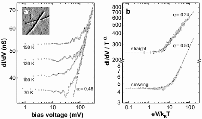
Figure 32: Differential conduction $dI/dV$ measured by Postma et al. [197] for carbon nanotubes. At low voltages or temperatures, Coulomb blockade effects dominate, but at higher temperatures or bias voltages, one probes the one-dimensional SFL behavior. Panel (a) shows the differential conductance as a function of bias voltage for various temperatures (note that these temperatures are relatively high, reflecting the fact that the electronic energy scales of the nanotubes is high). The effective exponent $\alpha$ for the large $V$ behavior is 0.48; since these data are for tunneling between two nanotubes, $\alpha=2\gamma_{c}$, so $\gamma_{c}\approx 0.24$ and $K_{c}\approx 0.27$. The predicted value is $K_{c}\approx 0.2$ [133]. The data in panel (b) show the differential conductance as a function of temperature at fixed bias for two nanotubes which cross, as well as for a single nanotube with a bend.

By contrast, at the tips of the nanotubes, surplus electronic charge can propagate in only one direction and, as a consequence, the tunneling is more restricted,

$$N_{tip}(\omega)\sim\omega^{\alpha_{tip}}~{}~{}~{}\mbox{ with }~{}\alpha_{tip}=(K_{c}-1)/4~{}.$$ (145)

By Fermi’s golden rule, the relevant exponents for (tip-tip) or (bulk-bulk) tunneling are $\alpha_{t-t}=(K_{c}-1)/2$ and $\alpha_{b-b}=2\gamma_{c}$ respectively. Bulk-bulk tunneling is achieved by arranging the nanotubes according to the crossing geometry depicted in the inset of Fig. 32 above. By extracting the value of the charge stiffness $K_{c}$ from each of the independent measurements of $\alpha_{t-t},\alpha_{b-b}$ for the two different geometries, a single consistent stiffness $K_{c}\approx 0.27$ was found [197], in good agreement with theoretical prediction. This is a beautiful realization of Luttinger Liquid physics!

Other, older, canonical realizations of Luttinger liquids include the Quantum Hall edge states. These represent a chiral spinless Luttinger liquid. Here, low lying energy states can only prevail at the edge of the sample, and, concurrently, disperse linearly about the Fermi energy. Edge states can attain macroscopic linear (perimeter) extent, and the tunneling experiments between such states [170, 110] have observed several features predicted theoretically [271, 132]. We refer the interested reader to the review articles by Schulz et al. [218] and Fisher and Glazman [96] for further details.

5 Singular Fermi-liquid behavior due to gauge fields

5.1 SFL behavior due to coupling to the electromagnetic field

Almost thirty years ago Holstein, Pincus and Norton [120] (see also Reizer [207]) showed that the coupling of electrons to the electromagnetic fields gives rise to SFL behavior. Since the typical temperatures where the effects become important are of the order of $10^{-15}$ $K$, the effect is not important in practice. But the theory is of considerable general interest.

If we work in the Coulomb gauge in which $\nabla\cdot{\bf A}=0$ for the electromagnetic ${\bf A}$ field, then the transverse propagator $D_{ij}^{0}$ in free space is given by

$$D_{ij}^{0}({\bf k},\omega)=\langle A_{i}A_{j}\rangle({\bf k},\omega)={{\delta_{ij}-\hat{k}_{i}\hat{k}_{j}}\over{c^{2}k^{2}-\omega^{2}-i\epsilon}}~{},$$ (146)

where $\epsilon$ is an infinitesimal positive number. The interaction of the electrons with the electromagnetic field is described by the coupling term

$${\bf j}\cdot{\bf A}+\rho A^{2}~{},$$ (147)

where ${\bf j}$ is the electron current operator and $\rho$ the density operator.

Quite generally in the Coulomb gauge, one finds from perturbation theory, or phenomenologically from the Maxwell equations, that the electromagnetic propagator in a metal can be written as

$$D_{ij}^{-1}=\left(D^{0}_{ij}\right)^{-1}-M\left(\delta_{ij}-\hat{k}_{i}\hat{k}_{j}\right)^{-1}~{}.$$ (148)

The perturbative diagrammatic expansion of $M$ is indicated in Fig. 33. The first term leads to a term proportional to the density while the second term is the first correction due to particle-hole excitations; in formulas, these terms yield

$$M(k,\omega)={{4\pi\alpha}\over{m}}\left(n+{{1}\over{m}}\int{{{\rm d}^{d}p}\over{(2\pi)^{d}}}{{[p^{2}-({\bf p}\cdot{\hat{\bf k}})^{2}][f_{p-k/2}-f_{p+k/2}]}\over{\omega-(\epsilon_{p-k/2}-\epsilon_{p+k/2})}}\right).$$ (149)

Here $n$ is the electron density, and $\alpha=1/137$ is the fine structure constant. For $\omega/k\rightarrow 0$ the two terms combined yield

$$M(k,\omega)\approx{{3\pi\alpha n}\over{m}}\left[4\left({{\omega}\over{kv_{F}}}\right)^{2}+2i{{\omega}\over{kv_{F}}}\right]~{}.$$ (150)

At small frequencies, this yields for the propagator $D$

$$D_{ij}({\bf k},\omega)\approx{{\delta_{ij}-\hat{k}_{i}\hat{k}_{j}}\over{i6\pi\alpha n{{\omega}\over{nkv_{F}}}+c^{2}k^{2}-i\omega}}~{},$$ (151)

which corresponds to an overdamped mode with dispersion $\omega\sim k^{3}$.

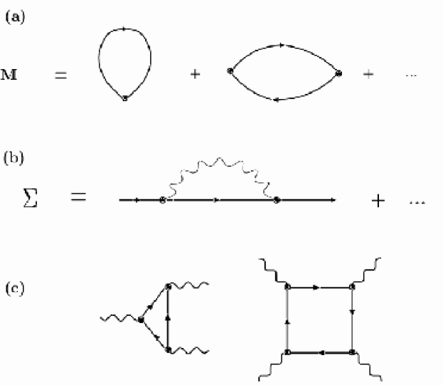
Figure 33: (a) The diagrams for M; (b) The diagram for the self-energy from the in the discussion of the SFL effect arising from the coupling of the electrons to the electromagnetic gauge fields; (c) Anharmonic interaction of fluctuations such as (c) are non-singular in the SFL problem of coupling of the electrons in metals to electromagnetic fields.

Before discussing how such a dispersion gives SFL behavior in three dimensions, it is instructive to point out that although (151) was obtained perturbatively, Maxwell’s equations ensure that the field propagator must generally be of this form at low frequencies and momenta. Indeed, for a metal we can write the current ${\bf j}$ as ${\bf j}=\sigma(k,\omega){\bf E}$; if we combine this with the Maxwell equation $\nabla\times{\bf H}={\bf j}+\partial{\bf E}/\partial t$ we easily find that the general form of the propagator is

$$D_{ij}({\bf k},\omega)={{\delta_{ij}-\hat{k}_{i}\hat{k}_{j}}\over{4i\pi\mu\omega\sigma({\bf k},\omega)+c^{2}k^{2}}}~{}.$$ (152)

Here $\mu$ is the diamagnetic permeability. For pure metals, the low-frequency limit is determined by the anomalous skin effect [5] and $\sigma({\bf k},0)\sim k^{-1}$. According to the expression (152), this $1/k$ behavior then implies that the dispersion at small frequencies generally goes as $\omega\sim k^{3}$ for a pure metal. For dirty metals, the fact that $\sigma(k,0)$ approaches a finite limit $\sigma_{0}$ at small wavenumbers, so for dirty metals there is according to (152) a crossover to a behavior $\omega\sim k^{2}$ at small wavenumbers.

Gauge invariance of the theory requires that the photon cannot acquire a mass (a finite energy in the limit $k\rightarrow 0$) in the interaction process with the electrons, and hence the form of Eq. (151) remains unchanged. Thus the anharmonic corrections to the photon propagator due to processes such as shown in Fig. 33(c) do not change the form of Eq. (151). The self-energy of the electrons due to photon exchange, Fig. 33(b), may now be calculated with confidence given the small coupling constant in lowest order. The leading contribution in $d=3$ is

$$\Sigma(k_{F},\omega)\sim\alpha(\omega\ln\omega+i\omega\mbox{sgn}\omega)$$ (153)

The momentum dependence, on the other hand, is nonsingular as a function of $k-k_{F}$.

The nonanalytic behavior of the self-energy as a function of frequency implies that the resistivity of a pure metal in $d=3$ is proportional to $T^{5/3}$ at low temperatures.

The simplicity and strength of the above example lies in the fact that the theory has no uncontrolled approximations, and the gauge-invariance of the photon field dictates the low-energy low-momentum behavior of the photon propagator $D_{ij}({\bf k},\omega)$. Moreover, vertex corrections are not important because the Migdal theorem is valid [195] when the frequency of fluctuations is very small compared to their momenta, as in $\omega\sim q^{3}$.

However, the SFL behavior as a result of the coupling to the electromagnetic field is not relevant in practice. This can most easily be argued as follows. For a Fermi gas, the entropy per particle is

$${{S}\over{N}}={{\pi^{2}mk_{B}^{2}T}\over{\hbar^{2}k_{F}^{2}}}~{},$$ (154)

while for the entropy for the electrons interacting with the electromagnetic field one finds from the above results [120]

$${{S}\over{N}}\approx{{2\pi^{2}\alpha\mu}\over{3}}{{T}\over{ck_{F}}}\ln\left({{\omega_{0}}\over{T}}\right)~{},$$ (155)

with

$$\omega_{0}={{c\epsilon_{F}}\over{\alpha\mu v_{F}}}~{}.$$ (156)

Upon comparing these two results, one concludes that the SFL effects start to become important for temperatures

$$T\stackrel{{\scriptstyle<}}{{\sim}}\omega_{0}e^{-{{3m^{*}ck_{B}^{2}}\over{2\alpha\mu\hbar^{2}k_{F}}}}~{}.$$ (157)

Since the numerical factor in the exponent is typically of order $10^{5}\mu^{-1}$ for ordinary metals, the temperature range one finds from this is of order $10^{-15}$ Kelvin for values of $\mu$ of order unity, according to this estimate. Note however that for pure ferromagnetic metals $\mu$ can be as large as $10^{4}$. Possibly, in some ferromagnets, the effects can become real.

5.2 Generalized gauge theories

The example of coupling to the electromagnetic field identifies one possible theoretical route to SFL behavior, but as we have seen the crossover temperatures that one estimates for this scenario are too small for observable physical properties. The smallness of the estimated crossover temperature is essentially due to the fact that the coupling to the electromagnetic field is determined by the product $\alpha v_{F}/c$, where $\alpha=1/137$ and typically $v_{F}/c={\mathcal{O}}(10^{-2})$. Motivated by this observation, many researchers have been led to explore the possibility of getting SFL effects from coupling to different, more general gauge bosons which might be generated dynamically in strongly correlated fermions. For a recent review with references to the literature, see [150, 179, 180]. The hope is that if one could consistently find such a theory in which the small factor $\alpha v_{F}/c$ arising in the electromagnetic theory is replaced by a term of order unity, realistic crossover temperatures might arise. Much of the motivation in this direction comes from Anderson’s proposal [24] of spin-charge separation and resonating valence bonds in the high-temperature superconductivity problem which we discuss in section 7.

The essence of approaches along these lines is most easily illustrated by considering electrons on a lattice in the case in which strong on-site (Hubbard-type) repulsions forbid two electrons to occupy the same site. Then each site is either occupied by an electron with an up or down spin, or by a hole. If we introduce fictitious fermionic creation and annihilation operators $f^{\dagger}$ and $f$ for the electrons and fictitious bosonic hole creation and annihilation operators $b^{\dagger}$ and $b$ for the holes, we can express the constraint that there can only be one electron or one hole on each lattice site by

$$\sum_{\alpha=1}^{2}f^{\dagger}_{i\alpha}f_{i\alpha}+b^{\dagger}_{i}b_{i}=1~{}~{}~{}~{}~{}\mbox{for each }i~{}.$$ (158)

With this convention, the real electron field $\psi_{i\alpha}$ can be written as a product of these fermion and boson operators

$$\psi_{i\alpha}=f_{i\alpha}b^{\dagger}_{i}~{}.$$ (159)

This expresses the fact that given the constraint (158), a real fermion annihilation at a site creates a hole. This way of writing the electron field may be motivated by the physics of the one-dimensional Hubbard model: there a local excitation may indeed be expressed in terms of a charged spinless holon and an uncharged spinon. In general, in a transformation to boson and fermion operators as in (159) there is some freedom with which operator we associate the charge and with which one the spin.

Whenever we split a single electron operator up into two, as in (159), then there is a gauge invariance, as the product is unchanged by the transformation

$$f_{i\alpha}(t)\longrightarrow e^{i\lambda(t)}f_{i\alpha}(t)~{},~{}~{}~{}~{}~{}b_{i}(t)\longrightarrow e^{i\lambda(t)}b_{i}(t)~{}.$$ (160)

We can promote this invariance to a dynamical gauge symmetry by introducing a gauge field ${\bf a}$ and writing the Hamiltonian in the continuum limit as

$${\mathcal{H}} = \int d{\bf r}\sum_{\sigma}~{}f^{\dagger}_{\sigma}\left(-{{i\nabla+{\bf a}}\over{2m_{f}}}\right)^{2}f_{\sigma}+(\phi-\mu_{f})f^{\dagger}_{\sigma}f+$$ (161)

$$\hskip 56.9055pt+\int d{\bf r}~{}b^{\dagger}\left(-{{i\nabla+{\bf a}}\over{2m_{b}}}\right)^{2}b+(\phi-\mu_{b})b^{\dagger}_{\sigma}b~{}.$$

Here $\phi$ is a Lagrange multiplier field which is introduced to implement the constraint (158). Note that the $\bf a$ field enters in much the same way in the Hamiltonian as the electromagnetic field usually does — indeed, a change in the individual $f$’s and $b$’s by a space dependent phase factor as in (160) can be reabsorbed into a change of ${\bf a}$. Note also the presence of the chemical potentials $\mu_{f}$ and $\mu_{b}$ to enforce that for a deviation of the (average) density $n$ from one per site, the density of holes is $1-n$ and of fermions is $n$.

The next step in the theory is to find the fluctuation propagator for the ${\bf a}$ field, as a function of $\mu_{f}$ and $\mu_{b}$. For finite $\mu_{f}$ and negative $\mu_{b}$ (bosons uncondensed), the fluctuation propagator is similar to that of the previous section but with $(\alpha v_{F}/c)$ replaced by a term of ${\mathcal{O}}(1)$. Spinon and holon self-energies can now be calculated and composition laws [126] are derived to relate physical correlation functions to correlation functions of spinons and holons.

Unfortunately, this very attractive route has turned out to be less viable than had been hoped. It is not clear whether the difficulties are purely technical; they are certainly formidable. The essential reason is that while photons have no mass and are not conserved, and hence can not Bose condense, in a gauge theory obtained by introducing additional bosons, the bosons generally can and will Bose condense because they do have a chemical potential. Bose condensation leads to a mass term in the propagator for the gauge fields. The singularities in the fermions due to the gauge fields then disappear. It is the analogue of the fact that superconductivity leads to the Meissner effect — there the emergence of the superconducting field breaks gauge invariance and leads to the expulsion of the magnetic field from the superconductor. The latter effect can also be thought of as being due to the generation of a mass term for the gauge fields.

Several variants of these ideas have been proposed with and without attempts to suppress the unphysical condensation through fluctuations [176]. The trouble is that such fluctuations tend to bind the spinons and holons and the happy situation in one dimension where they exist independently — being protected by (extra) conservation laws, see section 4.9 — is hard to realize. As usual, it appears that introduction of new quantum numbers requires new symmetries.

Interesting variants using the idea of spin-charge separation have recently appeared [220, 176].

6 Quantum Critical Points in fermionic systems

As mentioned in the introduction, quantum critical behavior is associated with the existence of a $T=0$ phase transition; of course, in practice one can only study experimentally the behavior at nonzero temperatures, but in this sense the situation is no different from ordinary critical phenomena: one never accesses the critical point itself, but observes the critical scaling of various experimentally accessible quantities in its neighborhood.

In practice, the most common situation in which one observes a quantum critical point is the one sketched in Fig. 1, in which there is a low temperature ordered state — a ferromagnetic state, antiferromagnetic state or charge density wave ordered state, for instance — whose transition temperature to the disordered state or some other ordered state goes to zero upon varying some parameter. In this case, the quantum critical point is then also the end point of a $T=0$ ordered state. However, sometimes the “ordered” state really only exists at $T=0$; for example in metal-insulator transitions and in quantum Hall effect transitions [232, 198]. A well-known example of this case in spin models is in two-dimensional antiferromagnetic quantum Heisenberg models with ”quantumness’ as a parameter $g$ [55], which do not order at any finite temperature, but which show genuine ordered phases at $T=0$ below some value $g<g_{c}$.

Although the question concerning the origin of the behavior of high temperature superconductors is not settled yet, there are strong indications, discussed in the next section, that much of their behavior is governed by the proximity to a quantum critical point.

One of the first formulations of what we now refer to as quantum critical behavior was due to Moriya [177, 178] and Ramakrishnan [174], who did an RPA calculation for a model of itinerant fermions with a Stoner-type instability to a ferromagnetic state. In modern language, their approach amounts to a $1/N$ expansion. Various other important contributions were made [37, 77]. The now standard more modern formulation, which we will follow, is due to Hertz [117]. A nice introduction can be found in the article by Sondhi et al. [232], and for a detailed expose we refer to the book by Sachdev [210]. See also the review by Continento [66].

6.1 Quantum critical points in ferromagnets, antiferromagnets, and charge density waves

A clear example of quantum critical behavior, and actually one for which one can compare with theoretical predictions, is summarized in Figs. 34-37. The figures show various data from [239] on the magnetic compound $MnSi$ [191, 192, 152, 161, 239]. Fig. 34 shows that for low pressures and temperatures, this compound exhibits a magnetic phase whose transition temperature $T_{c}$ vanishes as the pressure is increased up to $p_{c}=14.8~{}kbar$. This value of the pressure then identifies the quantum critical point. Fig. 35 shows that when the same data are plotted as $T_{c}^{4/3}$ versus pressure, the data fall nicely on a straight line except close to the critical pressure. This observed scaling of $T_{c}^{4/3}$ with $p-p_{c}$ away from $p_{c}$ is in accord with the behavior predicted by the theory discussed below. Actually the transition is weakly first order near $p_{c}$; so very detailed verification of the theory is not possible.

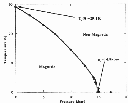
Figure 34: Magnetic phase diagram as a function of pressure of $MnSi$ [191, 192, 239]. From [239].

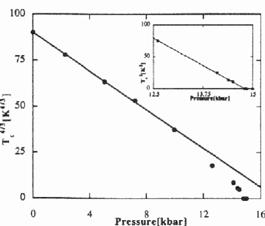
Figure 35: Power law dependence of the Curie-temperature as a function of pressure for $MnSi$. From [239].

Figure 36: $T$-dependence of $(\rho(T)-\rho_{T=0})$ near the critical pressure $p_{c}$ with and without an external magnetic field. From [239].

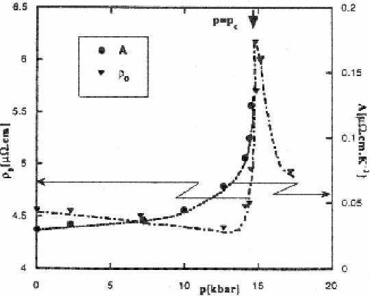
Figure 37: Evolution of $\rho_{0}$ and A under pressure, when the temperature dependence of the resistivity is fitted to $(\rho=\rho_{0}+AT^{2})$. From [239].

Fig. 36 shows data for the temperature dependence of $\rho-\rho_{0}$ near $p_{c}$, where $\rho_{0}$ is the residual low temperature resistivity. In the presence of a field of 3 Tesla, one observes the usual $\rho-\rho_{0}\sim T^{2}$ Fermi-liquid scaling, but at zero field the results are consistent with$\rho-\rho_{0}\sim T^{5/3}$ behavior predicted by the theory. But if we write the low temperature resistivity behavior as

$$\rho=\rho_{0}+AT^{\theta}$$ (162)

then both the residual resistivity $\rho_{0}$ and the amplitude $A$ are found to show a sharp peak at $p_{c}$ as a function of pressure — see Fig. 37. This behavior is not understood nor is the fact that the exponent $\theta$ does not appear to regain the Fermi-liquid value of 2 for significant values of $p>p_{c}$ (at $H=0$) and in a temperature regime where the theory would put the material in the quantum-disordered Fermi-liquid regime.

6.2 Quantum critical scaling

Before discussing other experimental examples of quantum critical behavior it is expedient to summarize some of the essential quantum critical scaling ideas.

As is well known, at a finite temperature transition, the critical behavior is classical and we can use classical statistical mechanics to calculate the correlation functions. This is so because due to critical slowing down the characteristic time scale $\tau$ diverges with the correlation length,

$$\tau\sim\xi^{z}~{}.$$ (163)

Near a critical point the correlation length $\xi$ diverges as

$$\xi\sim|T-T_{c}|^{-\nu}~{}.$$ (164)

The combination of these two results shows that critical slowing down implies that near any finite temperature critical point the characteristic frequency scale $\omega_{c}$ goes to zero as

$$\omega_{c}\sim|T-T_{c}|^{\nu z}~{}.$$ (165)

Therefore near any phase transition $\omega_{c}\ll T_{c}$, and as a result the phase transition is governed by classical statistical physics: the Matsubara frequencies are closely spaced relative to the temperature, the thermal occupation of bosonic modes is large and hence classical, etc.

In classical statistical mechanics, the dynamics is a slave to the statics; usually, the dynamical behavior is adequately described by time-dependent Landau-Ginzburg type of equations or Langevin equations which are obtained by building in the appropriate conservation laws and equilibrium scaling behavior [112]. At a quantum critical point, the dynamics must be determined a priori from the quantum-mechanical equations of motion.

The general scaling behavior near a $T=0$ quantum critical point can however be discussed with the formalism of dynamical scaling [112, 156], just as near classical critical points. Consider for example the susceptibility for the case of $MnSi$ that we considered above. The scaling ansatz for the singular part of the susceptibility

$$\chi(k,\omega,p)=\langle MM\rangle(k,\omega,p)$$ (166)

implies that near the critical point where the correlation length and time scale diverge, the zero-temperature susceptibility $\chi$ is a universal scaling function of the scaled momentum and frequency,

$$\chi(k,\omega,p)=\xi^{-d_{M}}{\Upsilon}(k\xi,\omega\xi_{t})~{},$$ (167)

where now

$$\xi\sim|p-p_{c}|^{-\nu}~{},~{}~{}~{}~{}~{}\xi_{t}\equiv\tau=\xi^{z}~{}.$$ (168)

This is just like the classical scaling with $T-T_{c}$ replaced by $p-p_{c}$. The reason for writing $\xi_{t}$ instead of $\tau$ is that in quantum statistical calculations, the “time-wise” direction becomes like an additional dimension, so that $\xi_{t}$ plays the role of a correlation “length” in this direction. However, the time-direction has both a long-time cutoff given by $1/k_{B}T$ and a short-time cutoff given by the high energy cutoff in the problem — exchange energy or Fermi-energy, whichever is smaller in the ferromagnetic problem. The short-time cutoff has its analog in the spatial scale. The long-time cutoff, which determines the crossover from classical to quantum behavior, plays a crucial role in the properties discussed below. The crucial point is that when $z\neq 1$, there is anisotropic scaling between the space and time-wise direction, and as we shall discuss below, this implies that as far as the critical behavior is concerned, the effective dimension of the problem is $d+z$, not $d+1$.

The exponent $d_{M}$ in (167) reflects that a correlation function like $\chi$ has some physical dimension which often is inevitably related to the spatial dimension. The dependence of critical properties on spatial dimensions must be expressible purely in terms of the divergent correlation length $\xi$. Often $d_{M}$ is fixed by dimensional considerations (in the language of field theory, it is then given by the “engineering dimension” of the field), but this may not be true in general. It must be so, however, if $\chi$ is a correlation function of a conserved quantity.

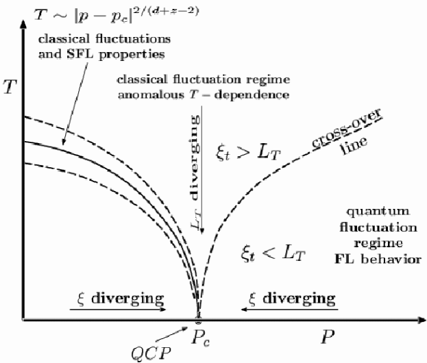
Figure 38: Generic phase diagram and cross-overs for quantum critical points with the various regimes indicated. $\xi$ is the correlation length at $T=0$; $L_{T}$ is the “thermal correlation length”.

Let us now address the finite temperature scaling, taking again the case of MnSi as an example. The various regimes in the $T$-$p$ diagram discussed below are indicated in Fig. 38. To distinguish these regimes it is necessary to define an additional quantity, the thermal length

$$L_{T}\equiv{{\hbar}\over{k_{B}T}}~{}.$$ (169)

$L_{T}$ corresponds dimensionally to a timescale. It marks the crossover between phenomena at long time scales which can be treated essentially classically from those on a shorter scale which are inherently quantum mechanical. Whenever $\xi_{t}<L_{T}$, the correlation length and time are finite and quantum mechanics begins to dominate. This is the regime on the right in the figure. Fermi-liquid behavior is expected in this regime. However, if one approaches the critical point $(T\!=\!0,~{}p\!=\!p_{c})$ from above along the vertical line, then $\L_{T}$ diverges but so does $\xi_{t}$. Moreover, $\xi_{t}$ diverges faster than $L_{T}$ since $z$ is usually larger $>1$. This means that the characteristic fluctuation energy and temperature are similar. So the behavior is quasiclassical throughout each correlated region down to zero temperature (In a path integral formulation [232, 210] one considers the model on a infinite strip whose width is finite in the timewise direction and equal to $L_{T}$. Hence for $\xi_{t}>L_{T}$ the model is fully correlated across the strip in this direction). This regime is therefore characterized by anomalous $T$ dependence in the physical quantities up to some ultra-violet cutoff. It is important to stress that this so-called “quantum critical scaling behavior” is expected in the observable properties in the whole region above $p_{c}$. So SFL can be observed over a whole range of parameter $p$ and temperatures between the left and right cross-over lines.

If one approaches the line of phase transitions to the ordered phase, which is marked with a solid line in the figure, one has a region with SFL properties dominated by classical fluctuations close to the transition. Millis [171] has corrected Hertz’s results [117] on this point, and has found that the critical temperature of the phase transition scales as $T_{c}\sim|p-p_{c}|^{z/(d+z-2)}$. Estimates of the classical critical region are also given. Results along similar lines may also be found in [65, 66].

If we include both the temperature and the parameter $p$, the scaling ansatz for the imaginary part of $\chi$ becomes

$$\chi^{\prime\prime}(k,\omega,p,T)~{}\sim~{}\xi^{-d_{M}}{\Upsilon}_{1}\left(k\xi,\omega\xi^{z},{{\omega}\over{T}}\right)~{}.$$ (170)

This can be rewritten in other forms depending on which experiment is being analyzed. For example, the above form is especially suitable for analysis as a function of $(p-p_{c})$. For analyzing data as a function of temperature, we may instead rewrite

$$\chi^{\prime\prime}(k,\omega,p,T)=L_{T}^{-d_{M}/z}{\Upsilon}_{2}\left(kL_{T}^{1/z},\omega L_{T},{{L_{T}}\over{\xi_{t}}}\right)~{},$$ (171)

and for analyzing data as a function of frequency

$$\chi^{\prime\prime}(k,\omega,p,T)=T^{-d_{M}/z}{\Upsilon}_{3}\left({{k}\over{T^{1/z}}},{{\omega}\over{T}},{{1}\over{T\xi_{t}}}\right)~{}.$$ (172)

Moreover, the scaling of the free energy ${\mathcal{F}}$ can be obtained from the argument that it is of the order of the thermal energy $k_{B}T$ per correlated volume $\xi^{d}$. Moreover, since $L_{T}$ acts as a finite cutoff for $\xi_{t}$ in the timewise direction, we then get the scaling

$${\mathcal{F}}\sim T\xi^{-d}\sim T(\xi_{t})^{-d/z}\sim T^{1+d/z}~{}.$$ (173)

By differentiating twice, this also gives immediately the specific heat behavior at low temperatures. In writing the above scaling forms, we have assumed that no “dangerously irrelevant variables” exist, as these could change $\omega/T$ scaling to $\omega/T^{\Delta}$ scaling.

In order to get the critical exponents and the cross-over scales, one has to turn to a microscopic theory. The theory for this particular case of the quantum critical point in $MnSi$ is essentially a Random Phase Approximation and proceeds along the following lines: (i) One starts with a model of interacting fermions; (ii) An ordering field $M(k,\omega)$ is introduced; (iii) One assumes the fermions can be eliminated near the critical point to get a free energy in terms of $M$ of the form

$${\mathcal{F}} = \int{\rm d}\omega\int{\rm d}^{d}k\chi^{-1}(k,\omega)|M(k,\omega)|^{2}+$$ (174)

$$\hskip 34.14322pt+\int{\rm d}\{\omega\}\int{\rm d}\{k\}~{}VM(k_{1},\omega_{1})M(k_{2},\omega_{2})Mk_{3},\omega_{3})M(k_{4},\omega_{4})$$

$$\hskip 62.59596pt\times~{}\delta(\omega_{1}+\omega_{2}+\omega_{3}+\omega_{4})\delta(k_{1}+k_{2}+k_{3}+k_{4})+\cdots$$

Note that this is essentially an extension of the usual Landau-Ginzburg-Wilson free energy to the frequency domain. Indeed, from here on one can follow the usual analysis of critical phenomena, treating the frequency $\omega$ on an equal footing with the momentum $k$.

The important result of such an analysis is that the effective dimension as far as the critical behavior is $d+z$, not $d+1$ as one might naively expect. Since $z\geq 1$ in all known examples, the fact that the effective dimension is bigger than $d+1$ reflects the fact that the correlation “length” $\xi_{t}$ in the timewise direction grows as $\xi^{z}$, i.e. faster than the spatial correlation length. Moreover, the fact that $z\geq 1$ implies that the effective dimension of a $d=3$ dimensional problem is always larger or equal than four. Since the upper critical dimension above which mean field behavior is observed equals four for most critical phenomena, one thus arrives immediately at the important conclusion that most quantum critical points in three dimensions should exhibit classical fluctuations with mean field scaling exponents! It also implies that the critical behavior can typically be seen over a large parameter or temperature range — the question of the width of the critical region, which normally is determined by the Ginzburg criterion, does not arise. On the other hand, questions concerning the existence of dangerously irrelevant variables, due for example to the scaling of the parameters $V$ in Eq. (174), do arise.

In order to judge the validity and generality of these results, it is important to keep in mind that they are derived assuming that the coefficients of the $M^{2}$, $M^{4}$ terms are analytic functions of $k$, $\omega$ and the pressure $p$, etc. This is completely in line with the usual assumption of analyticity of the bare coupling parameters in a renormalization group approach. This assumption may well be violated — in fact none of the impurity models discussed earlier can be treated along these lines: the fermions can not be integrated there, and if one attempts to apply the above procedure, one finds singular contributions to the bare coupling parameters. Later on we shall discuss a three-dimensional experimental example where this assumption appears to be invalid. Secondly, it is inherently an expansion about the nonmagnetic state, which can not apply in the ordered phase: In the ordered phase with nonzero magnetization, $M\neq 0$, there is a gap for some momenta in the fermionic spectra. This gap can not be removed perturbatively.

In a ferromagnet, the ground state susceptibility on the disordered side is given by

$$\chi^{-1}(k,\omega)=\left[(p-p_{c})+k^{2}+{{i\omega}\over{kv_{F}}}\right]~{}.$$ (175)

In the first two terms we recognize the usual mean field type behavior with a correlation length that diverges as $\xi\sim(p-p_{c})^{1/2}$, hence the critical exponent $\nu=1/2$. The last term, which describes Landau damping of the spin wave modes, is very special here as it arises from fluctuations of magnetization, a quantity which is conserved, i.e., commutes with the Hamiltonian. Therefore the characteristic damping rate must approach zero as $k\rightarrow 0$. Since at the critical point (175) leads to a damping $\omega\sim k^{3}$, the critical exponent $z=3$. According to the theory described above, the critical behavior at the quantum critical point $(T\!=\!0,\;p\!=\!p_{c})$ is therefore of the mean-field type for any physical dimension $d>1$, since the effective dimension $d+z>4$ for $d>1$.

The scattering of electrons off the long wavelength spin waves is dominated by small angle scattering, and it is easy to calculate the resulting dominant behavior of the self-energy of the electrons. Near the critical point the behavior of $\chi$ is very similar to the electromagnetic problem we discussed in section 5. Analogously, one also finds SFL behavior here: in $d=3$, $\Sigma(k_{F},\omega)\sim\omega\ln\omega+i|\omega|$ while in $d=2$ one obtains $\Sigma(k_{F},\omega)\sim\omega^{2/3}+i|\omega|^{2/3}$. Furthermore, for the resistivity one finds in three dimensions $\rho\sim T^{5/3}$ — this is consistent with the behavior found in MnSi in the absence of a field, see Fig. 36. Moreover, as we mentioned earlier, according to the theory, near the critical point $T_{c}$ should vanish as $|p-p_{c}|^{z/(d+z-2)}$; with $d=z=3$ this yields $T_{c}\sim|p-p_{c}|^{3/4}$. As we saw in Fig. 35, this is the scaling observed over a large range of pressures, except very near $p_{c}$. $ZrZn_{2}$ [111] is an example in which the Ferromagnetic transition is shifted to $T=0$ under pressure continuously. The properties are again consistent with the simple theory outlined. There is however trouble on the horizon [153]. The asymptotic temperature dependence for $p>p_{c}$ is not proportional to $T^{2}$, as expected. We will return to this point in sections 6.4.

For antiferromagnets or charge density waves the critical exponents are different. In these cases, the order parameter is not conserved, and the inverse susceptibility in these cases is of the form

$$\chi^{-1}(k,\omega)=\left[(p-p_{c})+(k-k_{0})^{2}+{{i\omega}\over{\Gamma}}\right]~{},$$ (176)

where $k_{0}$ is the wavenumber of the antiferromagnetic or charge density wave order. From this expression we immediately read off the mean field exponents $z=2$ and $\nu=1/2$. Since the effective dimension $d+z$ is above the upper critical dimension for $d=3$, the mean field behavior is robust in three dimensions. In $d=2$, on the other hand, the effective dimension $d+z=4$ is equal to the upper critical dimension, and hence one expects logarithmic corrections to the mean field behavior. Indeed, in two dimensions one finds for the self-energy [119] $\Sigma(\hat{{\bf k}}_{F},\omega)\sim\omega\ln\omega+i|\omega|$ (only)for those $\hat{{\bf k}}_{F}$ from which spanning vectors to other regions of the Fermi-surface separated by ${\bf k}_{0}$ can be found; the resistivity goes as $\rho(T)\sim T^{2}\ln T$ in this case. However, if several bands cross the Fermi-surface, as often happens in heavy fermions, Umklapp-type scattering may enforce the same temperature dependence in the resistivity as in the single particle self-energy, except at some very low crossover temperature. The physical reason for this dependence despite the fact that the soft modes are at large momentums (and therefore vertex corrections do not change the temperature dependence of transport relaxation rates) is that the set of $\hat{{\bf k}}_{F}$ usually covers a small portion of the Fermi-surface.

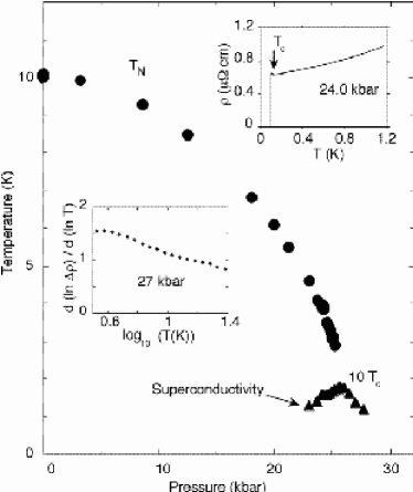
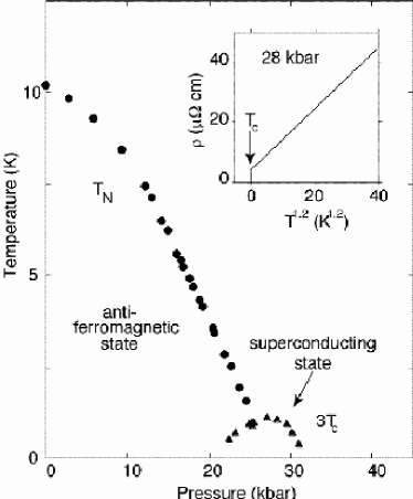
Figure 39: Left panel: Temperature-pressure phase diagram of high-purity single-crystal $CeIn_{3}$. A sharp drop in the resistivity consistent with the onset of superconductivity below $T_{c}$ is observed in a narrow window near $p_{c}$ the pressure at which the N el temperature $T_{N}$ tends to absolute zero. Upper inset: this transition is complete even below $p_{c}$ itself. Lower inset: just above $p_{c}$, where there is no N el transition, a plot of the temperature dependence of d($\ln\Delta\rho$ )/d($\ln$ T) is best able to demonstrate that the normal state resistivity varies as $T^{1.6\pm 0.2}$ below about 3 K. $\Delta\rho$ is the difference between the normal state resistivity and its residual value (which is calculated by extrapolating the normal-state resistivity to absolute zero). For clarity, the values of $T_{c}$ have been scaled by a factor of ten. Right panel: Temperature-pressure phase diagram of high-purity single-crystal $CePd_{2}Si_{2}$. Superconductivity appears below $T_{c}$ in a narrow window where the N el temperature $T_{N}$ tends to absolute zero. Inset shows the normal state a-axis resistivity above the superconducting transition varies as $T^{1.2\pm 0.1}$ over nearly two decades in temperature. The upper critical field $B_{c2}$ at the maximum value of $T_{c}$ varies near $T_{c}$ at a rate of approximately $-6T/K$. For clarity, the values of $T_{c}$ have been scaled by a factor of three, and the origin of the inset has been set at 5 K below absolute zero. Both plots are from Mathur et al. [161].

Fig. 39 shows the phase diagram of two compounds that order antiferromagnetically at low temperatures. The first one, $CeIn_{3}$ is a three-dimensional antiferromagnet. A superconducting phase intervenes at very low temperatures (note the different scale on which the transition to the superconducting phase is drawn), covering the region around the quantum critical point at a pressure of about 26 kbar. At this pressure, the normal state resistivity is found to vary as $\rho(T)\sim T^{1.6\pm 0.2}$ which is consistent with the theoretical prediction that at a quantum critical point dominated by antiferromagnetic fluctuations the resistivity should go as $\rho\sim T^{1.5}$. The right panel in Fig. 39 shows the phase diagram and resistivity data of the three dimensional antiferromagnet $CePd_{2}Si_{2}$; the data in this case are best fitted by $\rho\sim T^{1.2}$; this is consistent with the theoretical prediction $\rho\sim T^{1.25}$ which results if one has a $(k-k_{0})^{4}$ dispersion around the AFM vector $k_{0}$ in one direction and the usual $(k-k_{0})^{2}$ dispersion in the other two. No independent evidence for such dispersion is however available yet. In both of these cases, part of the region of superconductivity, in a region bounded by a line emanating from the QCP and going on to the antiferromagnetic to the normal state line, is expected to be antiferromagnetic as well.

These two compounds are also of interest because the phase diagram bears a resemblance to the phase diagram of the high- $T_{c}$ copper-oxide based superconductors in which the conduction electron density is the parameter varied — see. Fig. 49. Unlike the heavy fermion compounds where the ordered phase is antiferromagnetic, the order in copper-oxides near the QCP is not AFM. Its nature is in fact unknown. In the heavy fermion compounds superconductivity promoted by antiferromagnetic fluctuations is expected to be of the $d$-wave variety [175] as it is in the high- $T_{c}$ copper-oxide compounds.

6.3 Experimental Examples of SFL due to Quantum-Criticality: Open Theoretical Problems

We have discussed the observed quantum critical behavior in some system which is largely consistent with the simple RPA-like theoretical predictions. There are however quite a few experimentally observed signatures of singularities near QCPs, especially in heavy fermion compounds, which are not understood theoretically by the simple RPA theory of the previous subsection. In this section we present some prominent examples of these.

The experimental observations fall in two general categories, in both of which the low-temperature resistivity does not obey the power laws expected of Fermi-liquids: Compounds in which resistivity decreases from its limit at $T=0$ and those in which it increases. In both cases the $C_{v}/T$ is singular for $T\rightarrow 0$. It is reasonable to associate the former with the behavior due to impurities and the latter with the QCP properties of the pure system. But as we discussed in section 3.9 the QCP due to impurities requires tuning to special symmetries unlikely to be realized experimentally. As we will discuss, the effect of impurities without any special symmetries but coupling to the order parameter is expected to be quite different near the QCP of the pure system compared to far from it. Under some circumstances, it is expected to be singular and may dominate the observations.

We start with experiments in the second category. Figs. 40-42 shows several data sets for the heavy fermion compound $CeCu_{6-x}Au_{x}$ for various amounts of gold. This compound shows a low-temperature paramagnetic phase for $x<0.1$ and a low temperature antiferromagnetic phase for $x>0.1$. The specific heat data of Fig. 40 and the resistivity data of Fig. 42 show that while without $Au$, i.e. in the paramagnetic regime, the behavior is that of a Heavy Fermi-liquid metal, the alloy near the quantum critical composition $CeCu_{5.9}Au_{0.1}$ exhibits a specific heat with an anomalous

$$C_{v}\sim T\ln T~{}.$$ (177)

At the same composition, the resistivity shows a linear temperature dependence, and the susceptibility data in Fig. 41 show a $\sqrt{T}$ cusp. The anomalous behavior is replaced by Fermi-liquid properties both by a magnetic field and by increasing the substitution of copper by gold. The compound $YbRh_{2}S_{2}$ seems to have similar properties [243]. Related properties have also been found in $U_{2}Pt_{2}In$ [86, 87] and in $UPt_{3-x}Pd_{x}$ [74], $UBe_{13}$,$CeCu_{2}Si_{2}$, $CeNi_{2}Ge_{2}$ [235]. The SFL properties observed at the Mott-Insulator-Metal Transition in $BaVS_{3}$ [97] are also of related interest.

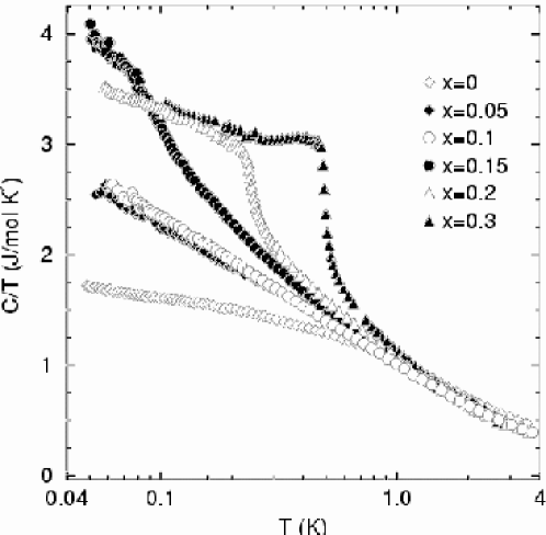
Figure 40: The specific heat $C/T$ of $CeCu_{6-x}Au_{x}$ versus $\log T$. From Löhneysen et al. [266, 267, 268].

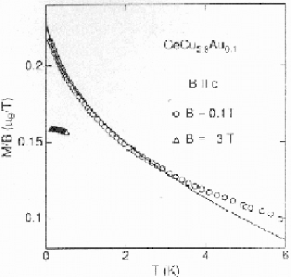
Figure 41: Susceptibility data for $CeCuAu$. From Löhneysen et al. [269].

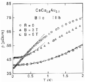
Figure 42: Resistivity data for $CeCuAu$. From Löhneysen et al. [269].

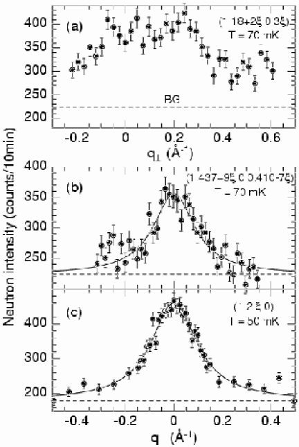
Figure 43: Neutron scattering data for $CeCu_{5.9}Au_{0.1}$, a compound which is close to a QCP. The figure shows $q$-scans along three different crystallographic directions, from top to bottom in the $a$, $b$ and $c$ directions for $\hbar\omega=0.1meV$. The figures shows that there is only a weak $q$-dependence along the rods ($q_{\perp}$), while transverse scans ($q_{||}$) shows well defined peaks with nearly the same line width. From Stockert et al. [236].

None of the quantum critical properties of the $CeCuAu$ compounds is consistent with any of the models that we have discussed. Information on the magnetic fluctuation spectra for $CeCu_{5.9}Au_{0.1}$ is available through neutron scattering experiments [215, 236]. The data shown in Fig. 43 show rod-like peaks, indicating that the spin fluctuations are almost two-dimensional at this composition. The neutron scattering data can be fitted by an expression for the spin susceptibility of the form

$$\chi^{-1}(k,\omega)=C\left[f(\delta k)+(-i\omega+aT)^{\alpha}\right]$$ (178)

with a function $f$ which is consistent with an effectively two-dimensional scattering,

$$f(\delta k)=b(\delta k_{\perp})^{2}+c(\delta k_{\parallel})^{4}~{}.$$ (179)

$\delta k_{\parallel}$ and $\delta k_{\perp}$ are the deviations from the AFM Bragg vector parallel and perpendicular to the c-axis in these tetragonal crystals. Further

$$a\approx 1~{},~{}~{}~{}~{}~{}\alpha=0.74\pm 0.1~{}.$$ (180)

At present, there is no room for this anomalous exponent $\alpha$ within known theoretical frameworks. However, if one accepts this particular form of $\chi$ as giving an adequate fit, the observed specific heat follows: at the critical composition, we expect the temperature scaling relation

$${\mathcal{F}}\sim T\xi_{\perp}^{-(d-1)}\xi_{\parallel}^{-1}\sim TT^{(d-1)\alpha/2}T^{\alpha/4}\sim T^{1+(d-1/2)\alpha/2}~{},$$ (181)

which immediately gives $C_{V}\sim d^{2}{\mathcal{F}}/dT^{2}\sim T$ for $\alpha=4/5$ with a plausible logarithmic multiplying factor.

The observed resistivity does not follow directly from the measured $\chi$; a further assumption is needed. The assumption that works is that fermions couple to the fluctuations locally, as in an effective Hamiltonian $\sim c^{\dagger}_{i,\sigma^{\prime}}c_{i,\sigma}S_{i,\sigma,\sigma^{\prime}}$. Then if the measured fluctuation spectra are that of some localized spins $S_{i}$, the single-particle self-energy is that due to exchange of bosons with propagator proportional to

$$\sum_{k}\chi({\bf k},\omega)\sim\ln(\omega)+i\;\mbox{sgn}\;(\omega).$$ (182)

This ensures that the single-particle relaxation rate as well as the transport relaxation rate is proportional to $T$. A major theoretical problem is why the non-local or ”recoil” terms in the interaction of itinerant fermions are irrelevant; i.e why is the effective Hamiltonian not

$$\Sigma_{k,q}c^{\dagger}_{k+q,\sigma}c_{k,\sigma^{\prime}}(S_{q}+S_{-q}^{\dagger})_{\sigma^{\prime},\sigma}.$$

Why has momentum conservation been legislated away?

The singularity of $\chi$ also raises the question whether the anharmonic processes, Fig. 33(c), which are benign and allow the elimination of fermions in the RPA theory, give singular contributions to $\chi$. Also can fermions really be eliminated in calculating the critical behavior.

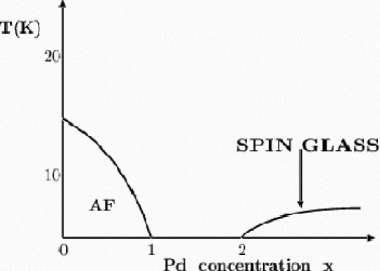
Figure 44: The phase diagram of $UCu_{5-x}Pd_{x}$. At low dopings and temperatures the system is in an antiferromgnetic phase. In the undoped sample ($x=0$): $T_{N}$= 15 K with a magnetization $\mu\simeq 1\mu_{B}$. For doping $x=1$ and 1.5 the specific heat $C_{v}/T\sim T$ (for $x=1$) while displaying weak logarithmic characteristics for $x=1.5$. Similarly, the susceptibility $\chi(T)\sim\ln T$ and $\chi\sim T^{-0.25}$ (for $x=1,~{}1.5$ respectively). Courtesy of M. C. Aronson.

As an example in the second category, we show in Fig. 44 the phase diagram of and some of the resistivity data of the heavy fermion compound $UCu_{5-x}Pd_{x}$. There are several other compounds in this category also; for a review we refer to [160, 165]. For a theoretical discussion of the scaling properties of some of this class of problems see [27].

For $x<1$, there is an (antiferromagnetic) ordered state at low temperatures, while for $x>2$, a spin-glass phase appears. At first sight, one would therefore expect possible SFL behavior only near the critical composition $x=1$ and near $x=2$. The remarkable observation however is that over a whole range of intermediate compositions, one observes anomalous behavior of the type [29, 30]

$$\rho=\rho_{0}-BT^{1/3}~{},~{}~{}~{}~{}~{}\chi\sim T^{-1/3}$$ (183)

The data for $\chi$ that show this power law behavior for $UCu_{3.5}Pd_{1.5}$ and $UCu_{1}Pd$ are shown in Fig. 45. The fact that this is genuine scaling behavior is independently confirmed [29, 30] from the fact that the frequency dependent susceptibility, measured by neutron scattering, shows a very good collapse of the data with the scaling assumption

$$\chi^{\prime\prime}(\omega,T)=T^{-1/3}\Upsilon\left({{\omega}\over{T}}\right)~{}.$$ (184)

In passing, we note that this as well as the result for $\chi$ in $CeCuAu$ are examples of an anomalous dimension, as the engineering dimension of the susceptibility $\chi$ is $1/energy$ — see the remark made just after Eq. (168).

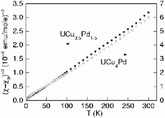
Figure 45: The temperature dependence of the static susceptibility of $\chi_{0}(T)$ for both $UCu_{4}Pd$ and $UCu_{3.5}Pd_{1.5}$, showing that for both compounds $\xi_{0}(T)$ has a low temperature divergence as $T^{-1/3}$. The measuring field is 1 Tesla. From Aronson et al. [29, 30].

Again, none of this behavior finds a clear explanation in any of the well-studied models. One is tempted to use the critical points of impurity models (see for example [69] and references therein), but runs into the difficulty of having to tune to special symmetries. The ideas of critical points of metallic spin-glasses (see for example [209] and also [219]), although theoretically appealing, are also not obviously applicable over such a wide range of composition. It must be mentioned however that NMR evidence does show clear evidence for the inhomogeneity in the singular part of the magnetic fluctuations in several heavy fermion compounds [41]. This has inspired models of varying sophistication (see [173] and references therein, and also [54]) in which the Kondo-temperature itself has a inhomogeneous distribution. It is possible to fit the properties with reasonable distributions but there is room for a deeper examination of the theoretical issues related to competition of disorder, Kondo effects and magnetic-interaction between the magnetic moments.

6.4 Special complications in heavy fermion physics

In heavy fermion compounds, there is often an additional complication that besets treating a QCP as a simple antiferromagnetic transition coupled to itinerant electrons. Often such materials exhibit magnetic order of the $f$-electrons (with magnetic moments of the ${\mathcal{O}}(1\mu_{B})$ per $f$-electron). Thus, such materials have local moments in the ordered phase; so the disappearance of the (anti)ferromagnetic order at a quantum critical point is accompanied by a metal-insulator transition of the $f$-electrons. This means that the volume of the Fermi-surface changes in the transition.

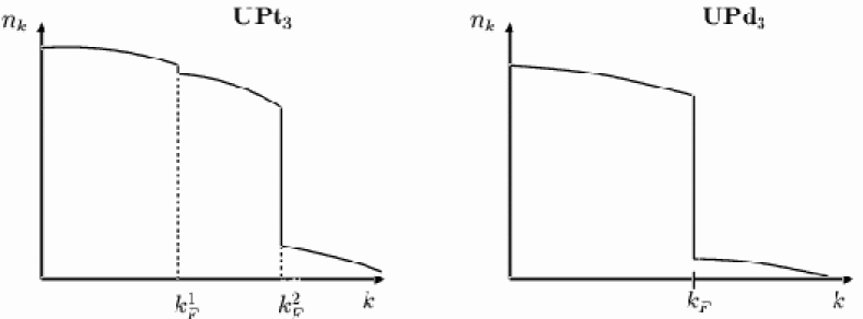
Figure 46: Schematic occupation number function $n_{k}$ for $UPt_{3}$ and for $UPd_{3}$.

We may illustrate the above scenario by comparing $UPt_{3}$, a Heavy fermion compound with effective mass of the order of 100, with $UPd_{3}$, an “ordinary” metal with effective mass of ${\mathcal{O}}(1)$ in which the f-electrons are localized. A schematic summary of the momentum occupation $n_{k}$ for the two cases is shown in Fig. 46: in the former $n_{k}$ is shown with two discontinuities, one small ${\mathcal{O}}(10^{-2})$ representing the large renormalisation in the effective mass of “$f$-electrons” while the other is close to 1 representing the modest renormalisation of $s$ and $d$-electrons. The other case, representative of $UPd_{3}$ has just one Fermi surface with a jump in $n_{k}$ of close to 1. The Fermi surface in the former encloses the number of electrons equal to the sum of the $f$ and $s$-$d$ electrons while the latter includes only the $s$-$d$ electrons. This is consistent with de Haas-van Alphen measurements as well as the band structures calculations of the two compounds; but the band-structure calculation must be done with the f-electrons assumed as itinerant in the former and part of the localized core in the latter. The magnetic transitions in heavy fermion compounds (with ordered moment of ${\mathcal{O}}(1\mu_{B})$) occurs through the conversion of itinerant $f$-electrons to localized electrons. So the Fermi surface on the two sides of the transition must switch between the two schematic representations in Fig. 46. The problem couples the ”metal-insulator transition” of the $f$-electrons to the magnetic fluctuations — those of itinerant electrons on one side and of interacting local moments on the other. The fluctuations of the metal-insulator transition and the Fermi surfaces is an important part of the problem. Some theoretical work with these ideas in mind is available [227]. Another possible approach is to generate an effective Hamiltonian for the heavy fermion lattice from a pairwise sum of the effective Hamiltonian deduced from the two-Kondo impurity problems discussed in section 3.9 and study its instabilities. The two impurity problem contains the rudiments of some of the essential physics.

In connection with the data in $CeCu_{6-x}Au_{x}$, we have discussed two important puzzles: the non-trivial exponent ${\em d_{M}/z}$ measured by $\chi(k,\omega)$, and the coupling of fermions to the local fluctuations alone for transport properties. In the other category (impurity-dominated) the first puzzle reoccurs; the second puzzle may be explained more easily since the measured fluctuation spectrum $\chi(k,\omega)$ is in fact $k-$independent. Both puzzles reoccur in the SFL phenomena in the cuprate compounds to be discussed in section 7.

6.5 Effects of impurities on Quantum Critical Points

As is well known, randomness can have an important effect on classical phase transitions. Two classes of quenched disorder are distinguished: First, impurities coupling quadratically to the order parameter [116] or, equivalently, impurities which may be used to define a local transition temperature $T_{c}(r)$; the second class concerns impurities coupling linearly to the order parameter [123]. The so-called Harris criterion, for the first class, tells us that the disorder is relevant, i.e. changes the exponents or turns the transition to a crossover, if the specific heat exponent $\alpha$ of the pure system is positive or, equivalently, if

$$d\nu-2<0~{}.$$ (185)

For application to QCP phenomena the value of $\nu$ to be used is different in the quantum fluctuation regime and the quasi-classical regime For the latter $\nu$ should be defined by the correlation length $\xi\sim(T-T_{c})^{-\nu_{1}}$ for a fixed $(p-p_{c})$ while deep in the former, near $T=0$ it should be defined by $\xi\sim(p-p_{c})^{-\nu_{2}}$. Accordingly the effect of disorder depends on the direction one approaches the QCP. Similarly the celebrated Imry-Ma argument [123] for linearly-coupled disorder can be generalized to QCP’s.

In problems of fermions, additional effects of disorder arise because the vertices coupling the impurity to the fermions can be renormalized due to the singularity in the fluctuation of the pure system [256]. Not too much work has been done along these lines. A simple example is the effect of magnetic impurities near a ferromagnetic transition [147]. The growth of the magnetic correlation length converts a single-channel Kondo effect to a multi-channel Kondo effect with a regime in which the singularities discussed in section 3.8 for the degenerate multi-channel Kondo effect may be realized without tuning any parameters [157]. This may be relevant to the deviations from the predictions of the pure case discussed here in the properties near the QCP in $MnSi$. Extensions of these ideas to antiferromagnetic and other QCP’s would be quite worthwhile.

7 The High-$T_{c}$ Problem in the Copper-Oxide Based Compounds

About $10^{5}$ scientific papers have appeared in the field of high-$T_{c}$ superconductors since their discovery in 1987. For reviews, see the Proceedings [164] of the latest in a series of Tri-annual Conferences or [106]. Although no consensus on the theory of the phenomena has been arrived at, the intensive investigation has resulted in a body of consistent experimental information. Here we emphasize only those properties which are common to all members of the copper-oxide family and in which Singular Fermi-liquid properties appear to play the governing role.

The high-$T_{c}$ materials are complicated, and many fundamental condensed matter physics phenomena play a role in some or other part of their phase diagram. As we shall see, the normal state near the composition of the highest $T_{c}$ shows convincing evidence of being a weak form of a SFL, a Marginal Fermi Liquid. Since the vertices coupling fermions to the fluctuations for transport in the normal state and those for Cooper pairing through exchange of fluctuations can be derived from each other, the physics of SFL and the mechanism for superconductivity in the cuprates are intimately related.

(a)          

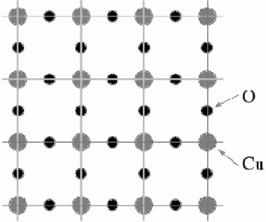
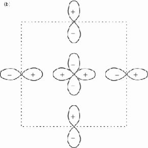
Figure 47: (a) Schematic structure of the copper-oxide $ab$-planes in $La_{2}CuO_{4}$. $Ba$ or $Sr$ substitution for $La$ in the parent compound $La_{2}CuO_{4}$ introduces holes in the $CuO_{2}$ planes. The structure of other high T_c materials differs only in ways which do not affect the central issues, e.g., it is oxygen doping in $YBa_{2}Cu_{3}O_{6+x}$ that provides planar holes. The magnetic moments of the planar copper atoms are ordered antiferromagnetically in the ground state of the undoped compounds. From [127]. (b) The “orbital unit cell” of the $Cu$-$O$ compounds in the $ab$ plane. The minimal orbital set contains a $d_{x^{2}-y^{2}}$ orbital of $Cu$ and $p_{x}$ and a $p_{y}$ orbital of oxygen per unit cell.

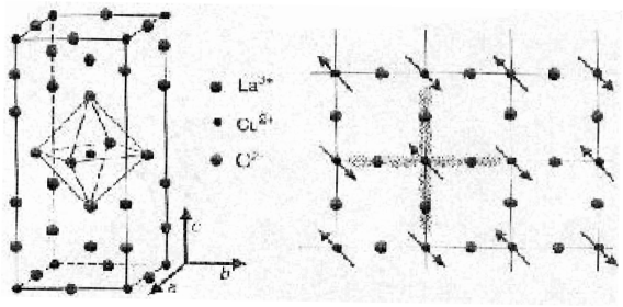
Figure 48: a) The crystal structure of $La_{2}CuO_{4}$. From [187]. Electronic couplings along the c direction are weak. b) Schematic of the $CuO_{2}$ plane. The arrows indicate the alignment of spins in the antiferromagnetic ground state of $La_{2}CuO_{4}$. Speckeled shading indicates oxygen $p_{\sigma}$ orbitals; coupling through these leads to superexchange in the insulating state.

7.1 Some basic features of the high-$T_{c}$ materials

A wide variety of $Cu$-$O$ containing compounds with different chemical formulae and different structures belong in the high-$T_{c}$ family. The common chemical and structural features are that they all contain two-dimensional stacks of $Cu$$O_{2}$ planes which are negatively charged with neutralizing ions and other structures in between the planes. The minimal information about the structure in the $Cu-O$ planes and the important electronic orbitals on Cu and on Oxygen is shown in Fig. 47. The structure of one of the simpler compound $La_{2-x}Sr_{x}CuO_{4}$ is shown in Fig. 48(a) with the $CuO_{2}$ plane shown again in Fig. 48(b). For $x=0$ the $CuO_{2}$ plane has a negative charge of 2 per unit cell which is nominally ascribed to the $Cu^{2+}(O^{2-})_{2}$ ionic configuration. Since $O^{2-}$ has a filled shell while $Cu^{2+}$ has a hole in the 3d shell, the $Cu$-$O$ planes have a half-filled band according to the non-interacting or one-electron model. But at $x=0$ the compound is an antiferromagnetic insulator with $S=1/2$ at the Copper sites. This is well known to be characteristic of a Mott-type insulator in which the electron-electron interactions determine the ground state. Actually [282, 251, 252] copper-oxide compounds at $x=0$ belong to the Charge-Transfer sub-category of Mott- insulators. But at $x=0$ the ground state and low-energy properties of all Mott-insulators are qualitatively the same. By substituting divalent $Sr$ for the trivalent $La$ in the above example, “holes” are introduced in the copper-oxide planes with density $x$ per unit cell.

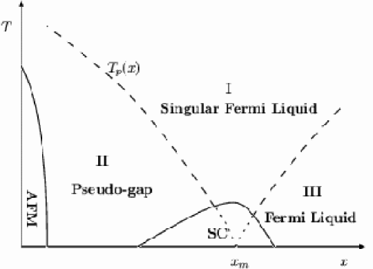
Figure 49: Generic phase diagram of the cuprates for hole doping. The portion labeled by AFM is the antiferromagnetic phase, and the dome marked by SC is the superconducting phase. Crossovers to other characteristic properties are marked and discussed in the text. Not shown is a low-temperature “insulating phase” in region II due to disorder.

Fig. 49 is the generic phase diagram of the $Cu$-$O$ compounds in the $T$-$x$ plane. In the few compounds with electron doping which have been synthesized properties vary with doping density in a similar way.

Antiferromagnetism disappears for $x$ typically less than 0.05 to be replaced by a superconducting ground state starting at somewhat larger $x$. The superconducting transition temperature is peaked for $x$ typically between 0.15 and 0.20 and disappears for $x$ typically less than 0.25. We will define $x_{m}$ to be the density for maximum $T_{c}$. Conventionally, copper-oxides with $x<x_{m}$ are referred to as underdoped, with $x=x_{m}$ as optimally doped and with $x>x_{m}$ as overdoped. Superconductivity is of the “$d$-wave” singlet symmetry.

The superconducting region in the $T$-$x$ plane is surrounded by three distinct regions: a region marked (III) with properties characteristic of a Landau Fermi-liquid, a region marked (I) in which (marginally) SFL properties are observed and a region marked (II) which is often called the pseudo gap region whose correlations in the ground state still remain a matter of conjecture. The topology of Fig. 49 around the superconducting region is that expected around a QCP. Indeed it resembles the phase diagram of some heavy fermion superconductors (see e.g. Fig. 39) except that region II has no long-range antiferromagnetic order — the best experimental information is that, generically, spin rotational invariance as well as (lattice) translational invariance remains unbroken in the passage from (I) to (II) in the $Cu$-$O$ compounds.

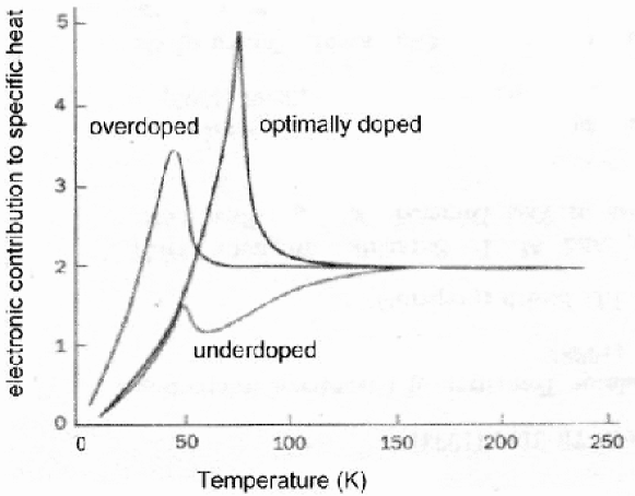
Figure 50: The electronic contribution to the specific heat as a function of temperature for underdoped, optimally doped and overdoped samples of Y_0.8Ca_0.2Ba₂Cu₃O_7-x. For optimally doped and overdoped samples the heat capacity remains constant as the temperature is lowered, then shows the characteristic features at the superconducting transition temperature $T_{c}$ and rapidly approaches zero in the superconducting state. For underdoped samples, however, the heat capacity starts to fall well above $T_{c}$ as the temperature is reduced, and there is only a small peak at $T_{c}$ indicating much smaller condensation energy than the optimal and overdoped compounds [154]. From [34].

The quantity $\gamma(T)\equiv C_{v}(T)/T$ and the magnetic susceptibility $\chi(T)$, which are temperature independent for a Landau-Fermi-liquid begin to decline rapidly [154] in the passage from region I to region II, which we will call $T_{p}(x)$, but without any singular feature. However, the transport properties — resistivity, Nuclear relaxation rate (NMR), etc. — show sharper change in their temperature dependence at $T_{p}(x)$. The generic deduced electronic contribution to the specific heat for overdoped, optimally-doped and underdoped compounds is shown in Fig. 50. The generic behavior for an underdoped compound for the resisitivity, Nuclear relaxation rate and Knight shift — proportional to the uniform susceptibility — is shown in Fig. 51. ARPES (Angle Resolved Photoemission) measurements show a diminution of the electronic density of states starting at about $T_{p}(x)$ with a four-fold symmetry: no change along the $(\pi,\pi)$ directions and maximum change along the $(\pi,0)$ directions. The magnitude of the anisotropic “pseudogap” is several times $T_{p}(x)$.

It is important to note that given the observed change in the single-particle spectra, the measured specific heat and the magnetic susceptibility in the pseudogap region are consistent with the simple calculation using the single-particle density of states alone. Nothing fancier is demanded by the data, at least at in its present state. Moreover, the transport properties as well as the thermodynamic properties at different $x$ can be collapsed to scaling functions with the same $T_{p}(x)$ as a parameter [275].

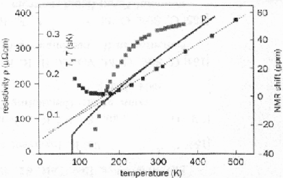
Figure 51: Signatures of the pseudogap in various transport properties for the underdoped compound $YBa_{2}Cu_{4}O_{8}$. At high temperatures the resistivity (solid line) decreases linearly with temperature. In the pseudogap region it drops faster with temperature before falling to zero at the superconducting transition temperature (about 85K). Similarly the NMR relaxation time displays characteristics of the optimum doped compounds above about 200 K (squares on dashed line) but deviates strongly from it in the pseudogap region. The NMR shift (top squares) also deviates from the temperature-independent behavior (not shown) below the inset of the pseudogap. Note that the pseudogap expresses itself as a sharper change with temperature in the transport properties compared to the equilibrium properties - specific heat and magnetic susceptibility. [45, 278, 10]. From [34].

7.2 Marginal Fermi Liquid behavior of the normal state

Every measured transport property in Region I is unlike those of Landau Fermi-liquids. The most commonly measured of these is the dc resistivity shown for many different compounds at the “optimum” composition in Fig. 52 including one with $T_{c}\approx 10K$. The resistivity is linear from near $T_{c}$ to the decomposition temperature of the compound. As shown in Fig. 51, in the “under-doped” region the departure from linearity commences at a temperature $\sim T_{p}(x)$ marked in Fig. 49. Similarly, the cross-over into region (III) shown in Fig. 49 is accompanied by Fermi-liquid like properties. Wherever measurements are available, every other measured transport property shows similar changes.

Figure 52: Resistivity as a function of temperature for various high temperature superconductors. From [38].

The different measured transport properties study the response of the compounds over quite different momentum and energy regions. For example, the Raman scattering studies the long wavelength density and current response at long wavelength but over a range of frequencies from low ${\mathcal{O}}(1cm^{-1})$ to high, ${\mathcal{O}}(10^{4}cm^{-1})$. On the other hand nuclear relaxation rate $T_{1}^{-1}$ depends on the magnetic fluctuations at very low frequencies but integrates over all momenta, so that the short wave-length fluctuations dominate. In 1989 it was proposed [253, 254] that a single hypothesis about the particle-hole excitation spectra captures most of the diverse transport anomalies.The hypothesis is that the density as well as magnetic fluctuation spectrum has an absorptive part with the following property:

$$\chi^{\prime\prime}(q,\omega)\left\{\matrix{=\ -\chi_{o}^{\prime\prime}~{}\omega/T~{},~{}~{}\ \mbox{for}\ \omega\ll T~{},\cr=\ -\chi_{o}^{\prime\prime}sgn(\omega)~{},~{}~{}~{}~{}~{}\mbox{for}\ \omega_{c}>\omega\gg T~{}.}\right.$$ (186)

Here $\chi_{o}^{\prime\prime}$ is the order of the bare single-particle density of states $N(0)$ and $\omega_{c}$ is an upper cut-off. The fluctuation spectrum is assumed to have only a weak momentum dependence, except at very long wavelength, where a $q^{2}$ dependence is required for fluctuations of conserved quantities like density or spin (in the absence of spin-orbit interactions). A form which implements these requirements for the conserved quantities with a rather arbitrary crossover function to get the different regimes of $\omega/T$ is

$$\chi^{\prime\prime}({\bf q},\omega)\ \sim\ {-xq^{2}\over\omega(\omega^{2}+\pi^{2}x^{2})},~{}~{}~{}\ \mbox{for}\ v_{F}q\ll\sqrt{\omega x},$$ (187)

where $x=\omega$ for $\omega/T\ll T$ and $x=T$ for $\omega/T\gg 1$.

Using the Kramers-Kronig relations, one deduces that the real part of the corresponding correlation functions have a $\log(x)$ divergence at all momenta except the conserved quantities where the divergence does not extend to $v_{F}q\geq x$. Thus compressibility and magnetic susceptibility are finite. (Besides (186), (187) analytic fluctuation spectra of the Fermi-liquid form is of course also present.)

The spectral function (186) is unlike those for a Landau Fermi-liquid discussed in section 2, which always have a scale — the Fermi-energy, Debye-frequency, or spin-wave energy, etc. — which is obtained from parameters of the Hamiltonian. Such parameters have been replaced by $T$. As we have discussed in section 6, this scale-invariance of (186) is characteristic of fluctuations in the quasi-classical regime of a QCP. Eq. (186) characterizes the fluctuations around the QCP: comparing with Eq. (170), the exponent $d_{M}/z=0$ and $1/z=0$. These are equivalent to the statement that the momentum dependence is negligibly important compared to the frequency dependence. This is a very unusual requirements for a QCP in an itinerant problem: the spatial correlation length plays no role in determining the frequency dependence of the critical properties.

The experimental results for the various transport properties for compositions near the optimum are consistent in detail with Eq. (186), supplemented with the elastic scattering rate due to impurities (see later). We refer the reader to the original literature for the details. The temperature independence and the frequency independence in Raman scattering intensity up to $\omega$ of ${\mathcal{O}}(1eV)$ directly follows from (187). Eq. (187) also gives a temperature independent contribution to the nuclear relaxation rate $T_{1}^{-1}$ as is observed for $Cu$ nuclei. The transport scattering rates have the same temperature dependence as the single-particle scattering rate. The observed anomalous optical conductivity can be directly obtained by using the continuity equation together with Eq. (187), or by first calculating the single-particle scattering rate and the transport scattering rate. The single-particle scattering rate is independently measured in ARPES experiments and provides the most detailed test of the assumed hypothesis.

To calculate the single-particle scattering rate, assume to begin with a constant coupling matrix element $g$ for the scattering of particles by the singular fluctuations. We shall return to this point in the section on microscopic theory. Then provided there is no singular contribution to the self-energy from particle-particle fluctuations, the graph in Fig. 53 represents the singular self-energy exactly. It is important to note that for this to be true, Eq. (187) is to be regarded as the exact (not irreducible) propagator for particle-hole fluctuations; it should not be iterated.

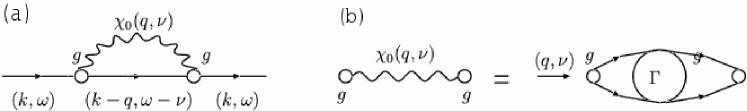
Figure 53: (a) Diagram for the singular contribution to the one-particle self-energy with the fluctuating $\chi(q,\nu)$. $g$’s are the vertices which in microscopic theory [255] is shown to have important momentum dependence, but which gives negligible momentum dependence to the self-energy. (b) For $\chi_{0}(q,\nu)$ which is momentum independent, a total vertex $\Gamma$ may sometimes be usefully defined, which has the same frequency dependence as Eq. (188) and which is also $q$-independent. The lines are the exact single-particle Green’s functions.

$\Sigma({\bf q},\omega)$ can now be evaluated straight forwardly to find a singular contribution,

$$\Sigma(\omega,q)\ \approx\ g^{2}(\chi_{o}^{\prime\prime})^{2}\ \left(\omega\ln{x\over\omega_{c}}-i\ {\pi\over 2}\ x\right)$$ (188)

for $x\ll\omega_{c}$ and $v_{F}|(q-k_{F})|\gg\omega_{c}$. The noteworthy points about (188) are:

(1) The single particle scattering rate is proportional to $x$ rather than to $x^{2}$ as in Landau Fermi-liquids.
(2) The momentum independence of the single-particle scattering rate.
(3) The quasi-particle renormalization amplitude

$$Z=\ \left(1-\lambda\ln\ {x\over\omega_{c}}\right)^{-1}$$ (189)

scales to zero logarithmically as $x\rightarrow 0$. Hence the name Marginal Fermi-liquid.
(4) The single-particle Green’s function

$$G(\omega,q)\ =\ {1\over\omega-(\epsilon_{q}-\mu)-\Sigma(q,\omega)}$$ (190)

has a branch cut rather than a pole. It may be written as

$${Z(x)\over\omega-(\tilde{\epsilon}_{q}-\tilde{\mu})-i/\tilde{\tau}}~{},$$ (191)

where $\tilde{\epsilon}_{q}$ is the renormalized single-particle energy:

$$\tilde{\epsilon}_{q}-\tilde{\mu}\ =Z(\epsilon_{q}-\mu)\ \approx\ Z{\bf v}_{F}\cdot({\bf q}-{\bf k}_{F})$$ (192)

for small $|q-k_{F}|$. Also $\tilde{\tau}^{-1}(x)=Z\;\mbox{Im}\Sigma(\omega)$, and the effective Fermi-velocity $\tilde{v}_{F}=Zv_{F}$ has a frequency and temperature dependent correction.
(5) The single-particle occupation number has no discontinuity at the Fermi-surface, but its derivative does, see Fig. 54. So the Fermi-surface remains a well-defined concept both in energy and in momentum space.

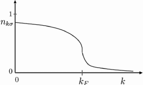
Figure 54: The $T=0$ distribution of bare particles in a marginal Fermi liquid. No discontinuity exists at $k_{F}$ but the derivative of the distribution is discontinuous.

The predictions of (190) have been tested in detail in ARPES measurements only recently. ARPES measures the spectral function

$$A(q,\omega)=-{1\over\pi}\ {\Sigma^{\prime\prime}(q,\omega)\over[\omega-(\epsilon_{q}-\mu)-\Sigma^{\prime}(q,\omega)]^{2}+[\Sigma^{\prime\prime}(q,\omega)]^{2}}~{}.$$ (193)

In ARPES experiments, the energy distribution curve at fixed momentum (EDC) and the momentum distribution curve at fixed energy (MDC) can both be measured. It follows from Eq. (193) that if $\Sigma$ is momentum independent perpendicular to the Fermi-surface, then an MDC scanned along ${\bf k}_{\perp}$ for $\omega\approx\mu$ should have a Lorentzian shape plotted against $({\bf k}-{\bf k}_{F})_{\perp}$ with a width proportional to $\Sigma^{\prime\prime}(\omega)/v_{F}(\hat{\bf k})$. For a Marginal Fermi Liquid (MFL), this width should be proportional to $x$. The agreement of the measured lineshape to a Lorentzian and the variation of the width with temperature are shown in Figs. 55. Fig. 56 shows the momentum width measured in different directions $\hat{\bf k}$. The Fermi-velocity $v(\hat{\bf k})$ is measured through the EDC with the conclusion that it is independent of $\hat{\bf k}$ to within the experimental errors. The data shows that the temperature dependence is consistent with linearity with a coefficient independent of $\hat{\bf k}$ although the error bars are huge near the $(\pi,0)$ direction. Besides the MFL contribution, there is also a temperature independent contribution to the width which is strongly angle-dependent, to which we will soon turn. The ambiguity of the temperature (and frequency) dependence near the $(\pi,0)$ direction is removed by the EDC measurements. In Fig. 56 EDC at the Fermi-surface in the $(\pi,\pi)$ direction and the $(\pi,0)$ directions are shown together with a fit to the MFL spectral function with a constant contribution added to $\Sigma^{\prime\prime}$. EDC’s have the additional problem of an energy-independent experimental background. This has also been added in the fit. In both directions $\Sigma^{\prime\prime}$ has a contribution proportional to $\omega$ with the same coefficient within the experimental uncertainty. In summary, the ARPES experiments give that

$$\Sigma^{\prime\prime}(k,\omega;T)\ \cong\ \Gamma(\hat{k}_{F})\ +\Sigma_{MFL}^{\prime\prime}(\omega,T).$$ (194)

The $(\omega,T)$-independent contribution $\Gamma(\hat{{\bf k}}_{F})$ can only be understood as due to impurity scattering [2]. Its dependence on $\hat{{\bf k}}_{F}$ can be understood by the assumption that in well-prepared samples, the impurities lie between the $Cu$-$O$ planes and therefore only lead to small angle scattering of electrons in the plane. The contribution $\Gamma(\hat{\bf k}_{F})$ at $\hat{\bf k}_{F}$ then depends on the forward scattering matrix element and the local density of states at $\hat{\bf k}_{F}$ which increase from the $(\pi,\pi)$ direction to the $(\pi,0)$ direction. This small angle contribution has several very important consequences: (i) relative insensitivity of residual resistivity to disorder, (ii) relative insensitivity of $d$-wave superconductivity transition temperature to the elastic part of the single-particle scattering rate [134], and (iii) most significantly relative insensitivity to the anomalous Hall effect and magneto-resistance. Such anomalous magneto-transport properties follow from a proper solution of the Boltzmann equation including both small-angle elastic scattering and angle-independent MFL inelastic scattering [260].

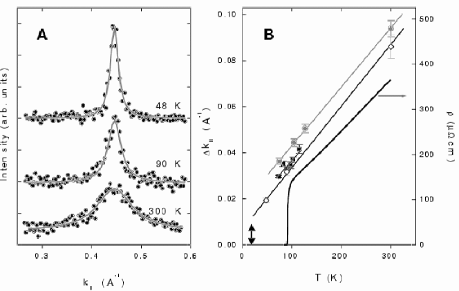
Figure 55: (a) Momentum distribution curves for different temperatures. The solid lines are Lorentzian fits. (b) Momentum widths of MDCs for three samples (circles, squares, and diamonds). The thin lines are $T$-linear fits which show consistency with Eqn.(193) and the MFL hypothesis. The resistivity (solid black line) is also shown. The double-headed arrow shows the momentum resolution of the experiment. From Johnson et al. [246].

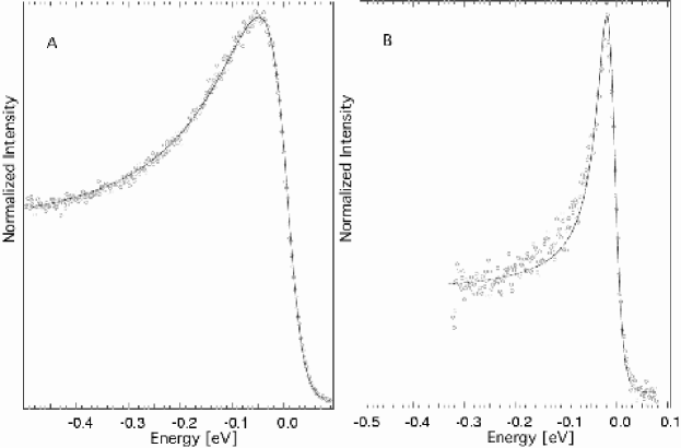
Figure 56: Fits of the MFL self-energy $\Gamma+\lambda\hbar\omega$ to the experimental data, according to (194). Estimated uncertainties of $\pm 15$% in $\Gamma$ and $\pm 25$% in $\lambda$. (a) A scan along the (1,0) direction, $\Gamma=0.12$, $\lambda=0.27$; (b) A scan along the (1,1) direction, $\Gamma=0.035$, $\lambda=0.35$. From Kaminsky and co-workers, [131].

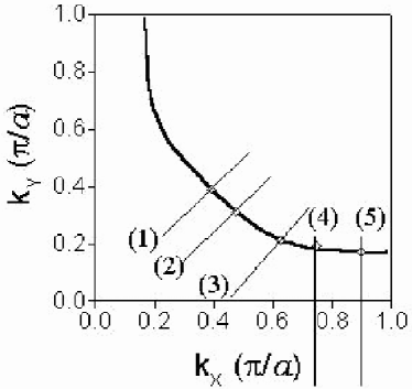
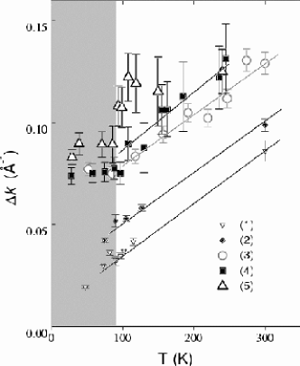
Figure 57: Left panel: Fermi surface of the optimally doped Bi2212, measure in the superconducting state. Indicated are the lines (1) to (5) on which the temperature dependence is measured in the experiments by Valla et al. [247]. Typical spectra are shown for line (2) in the normal (b) and superconducting state (c), as well as for line (4), in the normal (d) and superconducting state (c). Right panel: momentum widths as a function of temperature for different positions on the Fermi surface, obtained by fitting the Momentum Distribution Curves with Lorentzian lineshapes in the same experiments. Widths are measured at the Fermi level and at the leading edge, in the normal and in superconducting (grey region) state, respectively.

The momentum independence of the inelastic part of $\Sigma^{\prime\prime}$ is crucial to the SFL properties of the cuprates. Because the inelastic scattering to all angles on the Fermi-surface is the same, i.e. $s$-wave scattering, the vertex corrections to transport of vector quantities like particle current and energy current are zero. It follows that the momentum transport scattering rate measured in resistivity or optical conductivity and the energy transport rate measured in thermal conductivity have the same $(\omega,T)$ dependence as the single-particle scattering rate $1/\tau(\omega,T)$.

Recently far-infrared conductivity measurements [67] have been analyzed and shown to be consistent with $1/\tau(\omega,T)$ deduced from MFL including the logarithmic corrections.

As already discussed no singular correction to the magnetic susceptibility is to be expected on the basis of (186). But the specific heat should have a logarithmic correction so that

$$\gamma(T)=\gamma_{0}\left[1+\lambda\ln(\omega_{c}/T)\right]~{}.$$ (195)

Such a logarithmic correction has not yet been deciphered in the data presumably because the electronic specific heat in the normal state is less than ${\mathcal{O}}(10^{-2})$ of the total measured specific heat and must be extracted by a subtraction procedure which is not sufficiently accurate.

7.3 General Requirements on a Microscopic Theory

The MFL self-energy, Eq. (188), has been verified in such detail in its $(\omega,T,{\bf q})$ dependence that it is hard to see how any theory of $CuO$ compounds can be relevant to the experiments without reproducing it (or a very close approximation to it) in Region I of the phase diagram of Fig. 49. Such a scale-invariant self-energy is characteristic of the quasi-classical regime of a QCP and indeed the topological features of the phase diagram are consistent with their being a QCP at $x_{c}$ near the composition for the highest $T_{c}$ (Alternatively, a QCP in the overdoped region where $T_{c}$ vanishes is predicted in some approaches, like in [220]). To date, no way has been found to obtain Eq. (187) except through the scale-invariant form of fluctuations which is momentum independent $({\it z}\approx\infty)$ as in Eq. (186).

A consistent and applicable microscopic theory of the copper-oxides must show a QCP with fluctuations of the form (187). This is a very unusual requirement for a QCP in a homogeneous extended system for at least two reasons. First, the fluctuations must have a negligible ${\bf q}$-dependence compared to the frequency dependence, i.e. ${z}\approx\infty$ and second, the singularity in the spectrum should just have logarithmic form; i.e. there should be no exponentiation of the logarithm giving rise to power laws. Such singularities do arise, as we discussed in section 3, in models of isolated impurities under certain conditions but they disappear when the impurities are coupled; recoil kills the singularities. The requirement of negligible $q/\omega$ dependence runs contrary to the idea of critical slowing down in the fluctuation regime of the usual transitions, in which the frequency dependence of the fluctuations becomes strongly peaked at zero-frequency because the spatial correlation length diverges.

Another crucial thing to note is that any known QCP (in more than one dimension) is the end of a line of continuous transitions at $T=0$. Region II (at least at $T=0$) must then have a broken symmetry (This includes part of Region III, which is also superconducting). Experiments appear to exclude any broken translational symmetry or spin-rotational symmetry for this region although as discussed in section 7.1, a sharp change in transport properties is observed along with a four-fold symmetric diminution of the ARPES intensity for low energies at $T\approx T_{p}(x)$. If there is indeed a broken symmetry, it is of a very elusive kind; experiments have not yet found it.

A related question is how a momentum-independent $\chi({\bf q},\omega,T)$ can be the fluctuation spectrum of a transition which leads to an anisotropic state as in Region II. Furthermore, how can such a spectrum lead to an anisotropic superconducting state because it is unavoidable that $\chi({\bf q},\omega,T)$ of Eq. (187) which determines the inelastic properties in Region I also be responsible for the superconductive instability. After all, the process leading to the normal self-energy, Fig. 53, the superconductive self-energy, and the Cooper pair vertex, Fig. 58, are intimately related. Given Im$\chi({\bf q},\omega,T)$ the effective interaction in the particle-particle channel is

$$V_{pair}({\bf k},{\bf k}\pm{\bf q})\ =\ g^{2\ }Re\ \chi\ ({\bf q},\omega)~{}.$$ (196)

Re$\chi(q;\omega)$ is negative for all $q$ and for all $-\omega_{c}\leq\omega\leq\omega_{c}$. So we do have a mechanism for superconductive pairing in the Cu-O problem given by the normal state properties just as the normal state self-energy and transport properties of say $Pb$ tell us about the mechanism for superconductivity in $Pb$. In fact given that the normal state properties give that the upper cut-of frequency is of ${\mathcal{O}}(10^{3})$K and the coupling constant $\lambda\sim g^{2}N(0)$ is of ${\mathcal{O}}(1)$, the correct scale of $T_{c}$ is obtained. The important puzzle is, how can this mechanism produce $d$-wave pairing given that $\chi({\bf q},\omega)$ is momentum independent. How can one obtain momentum-independent inelastic self-energy in the normal state and a $d$-wave superconducting order parameter from the same fluctuations?

We summarize in the next section a microscopic theory which attempts to meet these requirements and answer some of the questions raised.

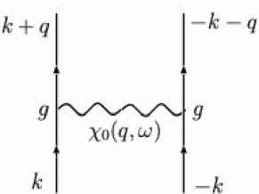
Figure 58: The Cooper pair-vertex and the normal state self-energy, Fig. 53, are intimately related.

7.4 Microscopic Theory

There is no consensus on even the minimum necessary model Hamiltonian to describe the essential properties in the phase-diagram, Fig. 49, of the $CuO$ compounds. It is generally agreed that, since other transition metal compounds do not share the properties of $CuO$ compounds, a model Hamiltonian with some rather special features is called for. Two such features are
(A) They are two-dimensional with an insulating antiferromagnetic ground state and spin $S=1/2$ per unit cell at half filling. Although not unique this feature is rare. If this is the determining feature, a two-dimensional Hubbard model is adequate. [24]. Even this model is not soluble in $d=2$.
(B) $CuO$ are the extreme limit of charge transfer compounds [282] in which charge fluctuations in the metallic state occur almost equally on Oxygen and Copper. Then the longer-range ionic interactions, which in magnitude are comparable to the on-site interactions have a crucial role to play in the low-energy dynamics in the metallic state through excitonic effects. A model with both $Cu$ and $O$ orbitals, hopping between them, and the excitonic interactions besides the on-site repulsions is then required [251, 252]. This is of course even harder to deal with than the Hubbard model.

Numerous attempts have been made using one or the other such models to obtain SFL behavior. We briefly discuss the motivations for the pursuit of model ${\em(A)}$ before summarizing in a little more detail the only attempt to obtain the phenomenlogical fluctuation spectrum of Eq. (186), and which relies on a model of type (B).

7.4.1 The Doped Hubbard Model

The investigations of the copper-oxide problem from this point of view asks some valid and deep questions [24]. How does a low concentration of holes move through the spin configurations in a two-dimensional model with restriction of zero double occupancy? We have sketched in section 4.8 the difficulties of connecting to the same problem in one dimension when the ground state at zero doping is an antiferromagnet. In fact analytic [213] and numerical [162] answers to the question for a single hole show the spectral weight of a heavy particle with an incoherent part composed of multiple spin-wave polaronic cloud. Simply extrapolated (a dangerous thing to do), a Fermi-liquid is expected. The larger zero-point fluctuations of the $S=1/2$ model, compared to a large spin model only change the relative weight of the coherent and the incoherent parts. But more subtle possibilities must be considered. The antiferromagnetic ground state of a Heisenberg $S=1/2$ model (or the undoped non-degenerate Hubbard model) in two-dimensions is close in energy to a singlet ground state. A possible description of such a state is as linear combination on a basis of singlet-bonds of pairs of spins. As noted earlier, such itinerant bond states have been termed Resonating Valence Bonds (by analogy to the ground state of Benzene like molecules). The massive degeneracy of the singlet bond-basis raises interesting possibilities. If the quantum fluctuations of spins were (significantly) larger than allowed by $S=1/2$, such states would indeed be the ground state, as they are in the one-dimensional model or two-dimensional models with additional frustrating interactions [6]. It is possible that by doping with holes in the $S=1/2$ Heisenberg model, the additional quantum fluctuations induce a ground state and low-lying excitations which utilize the massive degeneracy of RVB states. Especially intriguing is the fact that resonating valence ground state may be looked on as the projection of the BCS ground state to a fixed number of particles [24]. Furthermore in the normal state this line of reasoning is likely to lead to a SFL.

A specific proposal incorporating the RVB idea [136] relies on the ground state of the half-filled model to be localised dimers. Then defects in this state due to deviation from half-filling can plausibly support excitations which are charged spinless bosons. Further work on this idea may be found in [210, 176]. Related ideas were put forth in [80].

These are very attractive set of ideas and no proof exists that they are disallowed. We have already considered an implementation of these ideas in section 5.2 on generalized gauge theories. As discussed, controlled calculations using these ideas are hard to come by. Moreover, what theoretical results do exist do not correspond in a persuasive way to the experimental results on the copper-oxide materials.

One should take special note here of the idea of Anyon superconductivity which besides being a lovely theoretical idea, is founded on the solution to a well defined model, and has clear experimental predictions. Laughlin and collaborators [148, 130, 89] found a specific model with long-range four spin interactions for which his quantum hall wavefunction is the ground state. Therefore Time-reversal and Parity are spontaneously broken in this state. This state is superconducting. The predicted Time-reversal broken properties have not been observed experimentally [233].

An alternative idea from the microscopic characterization of these materials as doped Hubbard models is that a dilute concentration of holes in the Hubbard model is likely to phase separate or form ordered one-dimensional charge-density wave/spin-density wave structures [283, 284, 84]. There exists both empirical [242] and computational [272] support for this idea at least for a very dilute concentration of holes. For concentrations close to optimum compositions these structures appear in experiment to exist only at high energies with short correlation lengths and times and small amplitudes in the majority of copper-oxygen compounds. Their relation to SFL properties is again not theoretically or empirically persuasive.

7.4.2 The excitonic Interactions Model

This relies on a model of type ${\em(B)}$. A brief sketch of the calculations leading to a QCP and a MFL spectrum is given here. We refer the reader to [251, 253, 260] for details.

At half-filling the ground state and the low-lying excitations of such models are identical to the Hubbard model. But important differences can arise in the metallic state. Consider the one-electron structure of such models. The $O$-$O$ hopping in the lattice structure with $d_{x^{2}-y^{2}}$ orbitals in $Cu$ and $p_{x}$, $p_{y}$ orbitals on $O$, as shown in Fig. 47, produces a weakly dispersing “non-bonding” band while the $Cu$-$O$ hopping produces “bonding” and “anti-bonding” bands — see Fig. 59. We need consider only the filled non-bonding band and the partially filled anti-bonding bands shown in Fig. 59.

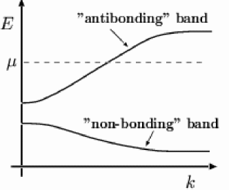
Figure 59: Three bands result from the orbitals shown in Fig. 47(b) in a one-electron calculation; two of these are shown. The chemical potential lies in the “anti-bonding” band and is varied by the doping concentration. The other band shown is crucial for the theory using excitonic effects as in [255].

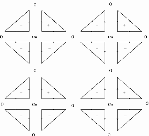
Figure 60: The current pattern in the time-reversal breaking phase predicted for Region II of the phase diagram.

In the mean-field approximation such an electronic structure together with the on-site interaction and the ionic interactions is unstable to an unusual phase provided the latter summed over the nearest neighbors is of the order or larger than the bandwidth. In this phase translational symmetry is preserved but time-reversal symmetry and the four-fold rotation symmetry about the $Cu$ sites is broken. The ground state has a current pattern, sketched in Fig. 60, in which each unit cell breaks up into four plaquettes with currents in the direction shown. The variation of the transition temperature with doping $x$ is similar to the line $T_{p}(x)$ in Fig. 38, so that there is a QCP at $x=x_{c}$. Experiments have been proposed to look for the elusive broken symmetry sketched in Fig. 60 [259].

The long-range interactions in the model also favor other time-reversal breaking phases which also break translational invariance. This is known from calculations on ladder models [189]. Such states have also been proposed for copper-oxide compounds [140, 121, 57].

Our primary interest here is how the mechanism of transition to such a phase produces the particular SFL fluctuation spectrum (187) in Region I of the phase diagram. The driving mechanism for the transition is the excitonic singularity, due to the scattering between the states of the partially filled conduction band $c$ and the valence band $v$ of Fig. 59. This scattering is of course what we considered in sections 3.5 and 4.9 for the problem of $X$-ray edge singularities for the case that the interband interaction $V$ in Eq. (55) is small and the valence band is dispersionless (i.e., the no recoil case). Actually, the problem is exactly soluble for the no-recoil case even for large $V$ [64]. For large enough $V$ the energy to create the exciton, $\omega_{ex}$, is less than the $v$-$c$ splitting $\Delta$. The excitonic lineshape is essentially the one sketched in Fig. 19(b) and given by Eq. (56) for $\omega>\omega_{ex}$, but $\delta$ is now the phase shift modulo $\pi$ which is the value required to pull a bound state below $\Delta$. The excitonic instability arises when $\omega_{ex}\to 0$.

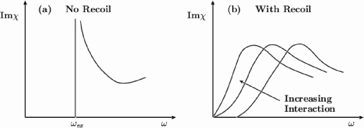
Figure 61: Sketch of the development of the particle-hole spectra in the microscopic model for the cuprates.

The effect of a finite mass or recoil on the excitonic spectra is to smoothen the edge singularity on the scale of the valence band dispersion between $k=0$ and $k=k_{F}$. The phase shift $\delta$ or the interaction energy $V$ no longer determines the low-energy shape of the resonance. $V$ does determine its location. The low-energy fluctuation spectra is determined by the following argument: Let us concentrate on $q=0$ which is obviously where Im$\chi_{ex}({\bf q},\omega)$ is largest. The absorptive part of a particle-hole spectra must be odd in frequency:

$$\mbox{Im}~{}\chi({\bf q},\omega)=-\mbox{Im}~{}\chi({\bf q},-\omega)~{}.$$ (197)

As $V$ increases, Im$\chi_{ex}(0,\omega)$ must shift its weight towards zero-frequency as shown in Fig. 61. Let us continue to denote by $|\omega_{ex}|$ the characteristic energy of the maximum in Im$\chi$. For $|\omega|$ small compared to $|\omega_{ex}|$, Im$\chi(0,\omega)\sim\omega$ while for $|\omega|$ large compared to $|\omega_{ex}|$, it is very slowly varying up to a cut-off $\omega_{c}$ on the scale of the Fermi-energy. Then by Kramers-Kronig transform the leading term in

$$\mbox{Re}\chi(0,\omega)\sim\ln\left(\omega_{c}/\max(\omega_{x},\omega)\right)~{}.$$ (198)

For any finite $|\omega_{ex}|$, Re$\chi$ is finite and there is no instability. Only for $|\omega_{ex}|\to 0$, i.e. Im$\chi(0,\omega)\to\mbox{sgn}\omega$, Re$\chi(0,\omega)$ is singular $\sim\ln|\omega|$ and there is an instability. Thus in an excitonic instability of a Fermi-sea with a dispersive valence band, the zero-temperature spectrum has the form $\chi(\omega,0)\sim\ln|\omega|+i\;\mbox{sgn}\;\omega$ at the instability. Given a parameter $p$ such that the instability occurs only at $p_{c}$, i.e. $\omega_{ex}(p\to p_{c})\to 0$, the generalization for finite temperature $T$ and momentum $q$ and $p\neq p_{c}$ is

$$\chi({\bf q},\omega) = \left[\left({{i\omega}\over{\mbox{max}(\omega,T,\omega_{ex}(p))}}+\ln{{\omega_{c}}\over{\mbox{max}(\omega,T,\omega_{ex}(p))}}\right)^{-1}\right.$$ (199)

$$\hskip 42.67912pt\left.+a^{2}q^{2}+(p_{c}(T)-p)\right]^{-1}~{}.$$

Here $\omega_{c}$ is the frequency cut-off of ${\mathcal{O}}(\Delta)$. Since the binding energy is ${\mathcal{O}}$(1eV), the size of the exciton, $a$, is of the order of the lattice constant. The ${\bf q}$’ dependence of (199) is negligible compared to the frequency dependence. The exponent ${z}$ is effectively infinite. At $p\approx p_{c}$ to logarithmic accuracy, the above expression (199) is identical to the phenomenological hypothesis (187).

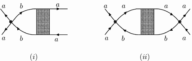
Figure 62: Singularity of interaction $\Gamma_{aaaa}$ between states ‘$a$’ near the chemical potential generated by the excitonic singularity between the states ‘$a$’ of the conduction band and states ‘$b$’ of the valence band. The excitonic singularity is indicated by the shaded block.

The effective low-energy interaction for states near the chemical potential, which is sketched in Fig. 62, is singular when the excitonic resonance is at low frequency. Here is an example of the mechanism mentioned under (v) in section 2.6 where the irreducible interaction obtained by integrating over non-perturbed high-energy states is singular. This is of course only possible when the interactions represented by the shaded block in Fig. 62 are large enough.

In relation to some of the questions raised about the phenemenology at the end of the last subsection, the momentum dependence of the vertex coupling the low energy fermions to the fluctuations in. Figs. 53 and 58 has been evaluated [258]. It is non-local with a form depending on the wave functions of the conduction and valence bands and the leading result is

$$g(k,k^{\prime})\sim\left(\sin(k_{x}a/2)\sin(k^{\prime}_{x}a/2)-\sin(k_{y}a/2)\sin(k^{\prime}_{y}a/2)\right).$$ (200)

Note that at $(k-k^{\prime})=0$ this is proportional to $[\cos(k_{x}a)-\cos(k_{y}a)]$. This is intimately related to the $d$-wave current distribution in the broken-symmetry phase predicted for region (II), shown in Fig. 60. Eq. (200) is such that that when diagram 53 is evaluated, the intermediate state momentum integration makes the self-energy depend very weakly on the incoming momentum. But when the pairing kernel of Fig. 58 is evaluated, its momentum dependent and exhibits attraction in the $d$-wave channel.

Similarly, as has been shown [258], the vertex of Eq. (200) leads to an anisotropic state with properties of the pseudo-gap state of region II below a temperature $T_{p}(x)$. The principal theoretical problem remaining with this point of view is that a transition of the Ising class occurs at $T_{p}(x)$at least in mean-field theory. This would be accompanied by a feature in the specific heat unlike the observations.

The microscopic theory reviewed above reproduces the principal features of the phase diagram Fig. 49 of the copper-oxide superconductors, and of the SFL properties. It also gives a mechanism for high temperature superconductivity of the right symmetry. Further confidence in the applicability of the theory to the cuprates will rest on the observation of the predicted current pattern of Fig. 60 in region II of the phase diagram .

8 The Metallic State in Two-Dimensions

The distinction between metals and insulators and the metal-insulator transition has been a central problem in condensed matter physics for seven decades. Despite the accumulated theoretical and empirical wisdom acquired over all these years, the experimental observation made in 1995 of a metal-insulator transition in two-dimensions [141] was a major surprise and is a subject of great current controversy. The theoretical work in the 1980’s [11, 90, 91, 92, 149, 14] on disordered interacting electrons pointed to a major unsolved theoretical problem in two dimensions. Infrared singularities were discovered in the scattering amplitudes which scaled to strong coupling where the theory is uncontrolled (The situation is similar to that after the singularities in the one- or two-loop approximations in the Kondo problem were discovered revealing a fascinating problem without providing the properties of the asymptotic low temperature state). However the problem was not pursued and the field lapsed till the new experiments came along.

The 1980’s theoretical work shows that this problem naturally belongs as a subject in our study of Singular Fermi-Liquids. We will first summarize the principal theoretical ideas relevant to the problem before the 1995 experiments. We then briefly summarize the principal results of these and subsequent experiments. Reviews of the experiments have appeared in [3, 16, 17]. There are two types of theoretical problems raised: the nature of the metallic state and the mechanism of the metal-insulator transition. We will address the former and only briefly touch on the latter.

8.1 The two-dimensional Electron Gas

We consider an electron gas with a uniform positive background with no complications arising from the lattice structure — this is how the many-electron problem was originally formulated: the Jellium model. This situation is indeed realized experimentally in MOSFETS (and heterostructures) in which an insulator is typically sandwiched between a metallic plate and a semiconductor — see Fig. 63. By applying an electric field a two-dimensional charge layer accumulates on the surface of the semiconductor adjacent to the insulator, whose density can simply be changed by varying the field strength (For details see [26]).. Similar geometries have been used to observe the Quantum Hall Effects and the metal-insulator transition by varying the density.

Typically we will be interested in phenomena when the average inter-electron distance is ${\mathcal{O}}(10)-{\mathcal{O}}(10^{2})\;nm$. The thickness of the insulating layer is typically more than $100\;nm$, so that the positive (capactive) charge on the insulator provides a uniform background to a first approximation. In $Si$ samles, surface roughness is the principle source of disorder at high densities, while at low densities (in the regime where the transition takes place) ionized impurity scattering dominates due to the fact that there is much less screening. In $GaAs$, remote impurity scattering dominates, and this scattering is mostly small-angle. This is the main reason the mobility in these samples is large.

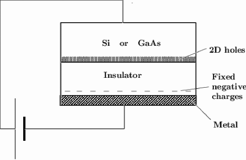
Figure 63: Sketch of a MOSFET. Holes (or electrons) are trapped at the interface of the semi-conductor and the insulator due to the band gap difference between them, the dipole layer and the applied electric field. Two-dimensional electrons (holes) may also be found by layered structures (heterostructures) of semi-conductors with different band gaps such as $GaAs$ and $AlGaAs$.

Neglecting disorder, the problem is characterized by $r_{s}$, defined as the ratio of the potential energy to the kinetic energy:

$$r_{s}=\frac{m\>e^{2}}{4\pi\epsilon\hbar^{2}\sqrt{\pi n}}~{}.$$ (201)

Here $n$ is the electron density, $m$ the band mass, and $\epsilon$ the background static dielectric constant. We can also write

$$\pi\>r^{2}_{s}\>a^{2}_{o}=\frac{1}{n}~{},$$ (202)

which expresses that $r_{s}$ is the radius of the circle whose area is equal to the area per conduction electron, measured in units of the Bohr radius $a_{0}$. For a two-valley band structure, as on the $110$ surface of $Si$, the kinetic energy is reduced and $r_{s}$ is twice that defined by Eqs. (201) and (202).

For $r_{s}\ll 1$, (the dense electron limit) the kinetic energy dominates and metallic behavior is expected. For $r_{s}\gg 1$, the potential energy dominates and a crystalline state (Wigner crystal) is expected. The best current numerical estimates put the transition to the crystalline state at $r_{sc}\approx 37$ [238]. The entropy at the transition is tiny, indicating that the radial distribution function for the liquid state at low densities is similar to that of the crystal for distances up to a few times $r_{s}a_{0}$.

It is important to note for our subsequent study that magnetism is always lurking close by. Reliable numerical calculations show that the magnetic state in the Wigner crystal near the critical density is determined by multiple-particle exchanges [46]. On the metallic side the energy of the ferromagnetic state is only a few percent above the unpolarized metallic or crystalline states for $r_{s}\approx r_{sc}$ [238]. Disorder is expected to make the metal-insulator state continuous. On the insulating side at $T\rightarrow 0$, the disordered Wigner crystal is expected to be glassy and have low-energy properties of a Coulomb glass [224]. On the metallic side fluctuations in the local density of electrons might be expected to lead to locally polarized magnetic states or possibly to some unusual frustrated magnetic states [56]. The perturbative calculations with disorder and interactions, already alluded to [90, 91, 92, 53] also hint at formation of magnetic moments in the metallic state. It is the interplay of such magnetic fluctuations with itinerancy which is one of the principal theoretical problem in understanding the metallic state.

8.2 Noninteracting Disordered Electrons: Scaling Theory of Localization

Detailed reviews on the material in this section may be found in [241, 149] [14, 125].

The concept of localization of non-interacting electrons for strong enough disorder was invented in 1958 by Anderson [18]. In one dimension all electronic states are localized for arbitrarily small disorder while in three dimension a critical value of disorder is required. That two dimensions is the marginal dimension in the problem was discovered through the scaling theory of localization.

The conceptual foundations for the scaling theory of localization were laid by Thouless and co-workers [240, 241] and by Abrahams et al. [1], and were developed formally by Wegner [270]. Abrahams et al. [1] also made predictions which could be tested experimentally. Thouless noted first of all that the conductance $G$ of a hypercube of volume $L^{D}$ in any dimension $d$ is dimensionless when expressed in units of $(e^{2}/h)$, thus defining a scale-independent quantity

$$g=G/\left(e^{2}/h\right).$$ (203)

Next, he argued that $g$ for a box of linear size $2L$ may be obtained from the properties of a box of size L and the connection between two of them. The conductance of a box of size $L$ itself increases with the transition amplitude $t$ between energy levels in the two boxes and decreases with the characteristic width of the distribution of the energy levels in the boxes $\Delta W(L)$ due to the disorder,

$$g(L)\approx f\left(\frac{\Delta t(L)}{\Delta W(L)}\right)~{}.$$ (204)

For weak-Gaussian disorder, the bandwidth may be expected to be proportional to the square-root of the number of impurities in the box, so $\Delta W(L)\sim L^{d/2}$. The transition amplitude $t$ is obtained by the hopping between near-neighbors near the surface of the boxes of size $L$. It is therefore proportional to the surface area $L^{d-1}$. Thus

$$g(L)=f\left(L^{(d-2)/2}\right)\>.$$ (205)

Now, in three dimensions the conductivity should approach a constant for large $L$ (Ohm’s law!), and hence the conductance should scale as $L$. This implies that the scaling function $f(x)$ should go for large $L$ as $f(x)\sim x^{2}$. Note that while for $d>2$ the $g$ therefore increases with increasing $L$ while for $d<2$ the large $L$ behavior is determined by the small argument behavior of the scaling function, while $d=2$ is the marginal dimension.

In a very influential paper, Abrahams et al. [1] analyzed the $\beta$-function of the RG flow

$$\beta(g)\equiv d(\ln g)/d(\ln L)~{},$$ (206)

and showed by a perturbative calculation in $1/g$ that

$$\beta(g)=\left(d-2\right)-\frac{1}{\pi^{2}}\>\frac{1}{g}~{},$$ (207)

where the first part comes from Eq. (205) with $f(x)\sim x^{2}$.

For small enough $g$ (i.e. for large disorder) we expect exponential localization $g(L)\sim e^{-L/\zeta}$, where $\zeta$ is the localization length, so that $\beta(g)\sim(-L/\zeta)$. The smooth connection between the perturbative result (207) for large $g$ and the exponentially localized solution at small $g$ is shown in Fig. 64. While for $d=3$ (or any $d>2$), a critical disorder $g_{c}$ is required for localization, in $d=2$ states are asymptotically localized for any disorder for non-interacting fermions. The characteristic value of the localization length in $d=2$ is estimated from the perturbative solution:

$$g(L)=g_{o}-\frac{1}{\pi^{2}}\>\ln\left(\frac{L}{\ell}\right)~{},$$ (208)

where $g_{o}$ is the dimensionless conductance at $L\approx\ell$. In conventional Boltzmann transport theory $g_{o}=(e^{2}/2\pi\hbar)k_{F}\ell$. $\zeta$ is of the order of the value of $L$ at which the correction term is of order $g_{0}$, so that

$$\zeta\approx\ell\exp\>\left(\frac{\pi}{2}k_{F}\ell\right)~{}.$$ (209)

At $T\rightarrow 0$, the sample size of a sample with $k_{F}\ell\gg 1$ has to be very large indeed for weak localization to be observable.

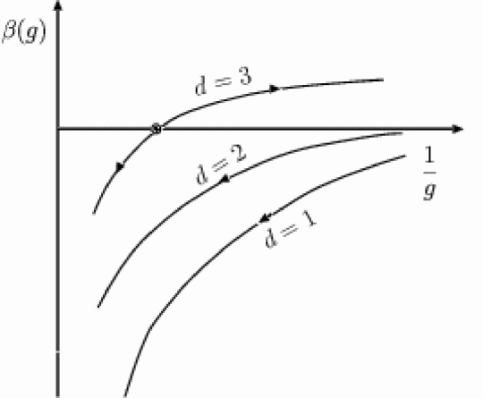
Figure 64: The scaling function for non-interacting electrons with disorder deduced by Abrahams et al. [1].

The theory described above must be modified at finite temperatures due to inelastic scattering. If the inelastic scattering rate is much less than the elastic scattering rate, $\tau^{-1}_{in}\ll\tau^{-1}$, localization effects are cut off at a length scale $L_{Th}(T)$, the Thouless length scale:

$$L_{Th}=\left(D\tau_{in}\right)^{1/2}$$ (210)

where $D=(v^{2}_{F}\tau/d)$ is the (Boltzmann) diffusion constant. However as noted by Altshuler, Aronov and Khmelnitski [12, 13], the correct scale for the cut-off is $\tau^{-1}_{\phi}$, the phase breaking rate. In an individual collision the energy change $\Delta E$ may be such that the phase changes only by a very small amount, $\tau_{in}\Delta E\ll 2\pi$. The phase breaking time is then longer and is shown to be given by $\tau_{\phi}\sim(\Delta E\>\tau_{in})^{-2/3}\>\tau_{in}$. The $T=0$ theory with

$$L_{\phi}=\left(D\tau_{\phi}\right)^{1/2}$$ (211)

replacing $L$ then gives the finite temperature scaling behavior to which experiments may be compared.

The characteristic temperature $T_{x}$ at which weak-localization effects become prominent may be estimated in a manner similar to (208),

$$T_{x}\tau_{\phi}(T_{x})=\exp\>\left(-\pi k_{F}\ell\right)~{}.$$ (212)

This expression puts useful bounds on the temperatures required to observe weak localization.

Eq. (207) is derived microscopically by considering repeated backward scattering between impurities. It can also be derived by considering quantum interference between different paths to go from one point A to another B [40]. The total probability $\Omega$ for this process is

$$\Omega=\left|\sum_{i}a_{i}\right|^{2}=\sum_{i}\left|a_{i}\right|^{2}+\sum_{i\neq j}a_{i}^{*}a_{j}~{},$$ (213)

where $a_{i}$ is the amplitude of the $i$-th path. The second term in Eq. (213) is non-zero only for classical trajectories which cross, for example at the point O in Fig. 65. The probability of finding a particle at the point $O$ is increased from $2|a_{i}|^{2}$ to

$$|a_{1}|^{2}+|a_{2}|^{2}+2\>Re\;a^{*}_{1}a_{2}=4|a_{1}|^{2}~{},$$ (214)

because the two paths are mutually time-reversed. Increasing this probability of course leads to a decrease in the probability of the particle to arrive at $B$, and hence to a decrease in the conductivity.

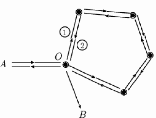
Figure 65: Interfering (time-reversed) parts in elastic scattering off a fixed set of impurities. The probability for the particle to arrive at B is reduced because of the enhance probability for the particle to arrive back at A, as a result of interference.

This argument makes clear why the interfering paths must be shorter than the phase relaxation rate due to inelastic processes and why magnetic impurities or a magnetic-field which introduces phase-shift between two otherwise time-reversed paths suppress weak-localization. In two-dimensions [14]

$$\sigma(H,T)-\sigma(O,T)=\frac{e^{2}}{2\pi^{2}\hbar}\left[\psi\left(\frac{1}{2}+\frac{1}{x}\right)+\ln x\right]~{},$$ (215)

where $\psi$ is the digamma function and

$$x=4L^{2}_{\phi}\>eH/\hbar c\equiv\left(L_{\phi}/L_{H}\right)^{2}\>.$$ (216)

The quantity in brackets in (215)is equal to $x^{2}/24$ for $x\rightarrow 0$ and to $\ln(x/4)-\gamma$ for $x\rightarrow\infty$.

Spin-orbit scattering preserves time-reversal symmetry but spin is no longer a good quantum number. The spins are rotated in opposite directions in the two self-intersecting paths of Fig. (65) if the impurities are spin-orbit scatters [14, 149]. This has been shown to lead to an average overlap of the spin-function of $-\frac{1}{2}$ (because a rotation by $2\pi$ of wave function of a spin $1/2$ particle leads to a wave function of opposite sign). The correction to the $\beta$-function of Eq. (207) due to this effect is

$$\frac{1}{2\pi^{2}}\>\frac{1}{g}~{}.$$ (217)

This effect tends to enhance the conductivity.

8.3 Interactions in Disordered Electrons

Fermi-liquid theory for interacting electrons survives in three dimensions in the presence of a dilute concentration of impurities [42]. Some noteworthy differences from the pure case are:

1. Because of the lack of momentum conservation, the concept of a Fermi-surface in momentum space is lost but it is preserved in energy space, i.e., a discontinuity in particle occupation as a function of energy occurs at the chemical potential. Momentum of particles may be defined after impurity averaging. General techniques for calculating impurity-averaged quantities are well developed; see for example [4, 42]. Here and subsequently in this chapter the self-energies, vertices etc. refer to their form after impurity averaging.

2. In the presence of impurities, the density-density correlation (and spin-density correlation, if spin is conserved) at low frequencies and small momentum must have a diffusive form (This is required by particle-number conservation and the continuity equation)

   $$\pi(q,\omega)=\kappa\>\frac{Dq^{2}}{i\omega+Dq^{2}}~{},~{}~{}~{}~{}~{}~{}q\ll\ell^{-1}~{}\mbox{and}~{}\omega\ll\tau^{-1}~{}.$$ (218)

   Here $\kappa=dn/d\mu$ is the compressibility and $D$ is the diffusion constant. For non-interacting electrons $D=\frac{1}{3}v^{2}_{F}\tau$. Interactions renormalize $D$ and $\kappa$ [42]. In the diagrammatic representation used below, the diffusive propagator is shown by a cross-hatched line connecting a particle and a hole line as in Fig. 66.

3. Because of statement 1, the impurity-averaged single-particle spectral function at a fixed $\bf{k}$ is spread out over an energy $\Gamma$, so that for frequencies within a range $\Gamma$ of the chemical potential, it has both a hole-part (for $\omega<\mu$) and a particle part (for $\omega>\mu$). This is an important technical point in microscopic calculations.

4. The Ward-identities relating the coupling of vertices to external perturbations change for the coupling to unconserved quantities (For the pure case they are given in section 2.6). For example no Ward-identity can be derived for the vertex needed for the conductivity calculation, i.e. $Lim_{\omega\rightarrow 0}\>Lim_{q\rightarrow 0}\>\Lambda^{impure}_{\alpha}$, because current is not conserved.

   $$Lim_{q\rightarrow 0}\>Lim_{\omega\rightarrow 0}\>\Lambda^{impure}_{\alpha}=\frac{k_{\alpha}}{m}-\frac{\partial\Sigma(k,\omega)}{\partial k_{\alpha}}$$ (219)

   holds because after impurity averaging momentum is conserved. But microscopic calculations show that at least when Fermi-Liquid theory is valid (Cf. section 2.4)

   $$Lim_{\omega\rightarrow 0}\>Lim_{q\rightarrow 0}\>\Lambda^{impure}_{\alpha}=Lim_{q\rightarrow 0}\>Lim_{\omega\rightarrow 0}\>\Lambda^{impure}_{\alpha}~{}.$$ (220)

   Indeed, if this were not so, one would not get a finite d.c. conductivity at $T=0$ for a disordered metal in $d=3$. An argument for this is as follows: Normally, we calculate the conductivity by first taking the limit $q\to 0$ and then the limit $\omega\to 0$, as on the left side of (220). In practice, however, even when we apply a homogeneous field to a system, the electrons in a disordered medium experience a field which varies on the scale of the distance between the impurities, and so the physically relevant limit is the one on the right hand side of (220), where the limit $\omega\to 0$ is taken first. But the validity of (220) appears not to extend to the case of Singular Fermi Liquids, at least for the present case where the singularities are $q$-dependent. This is one of the important difficulties in developing a consistent theory for disordered interacting electrons in $d=2$.

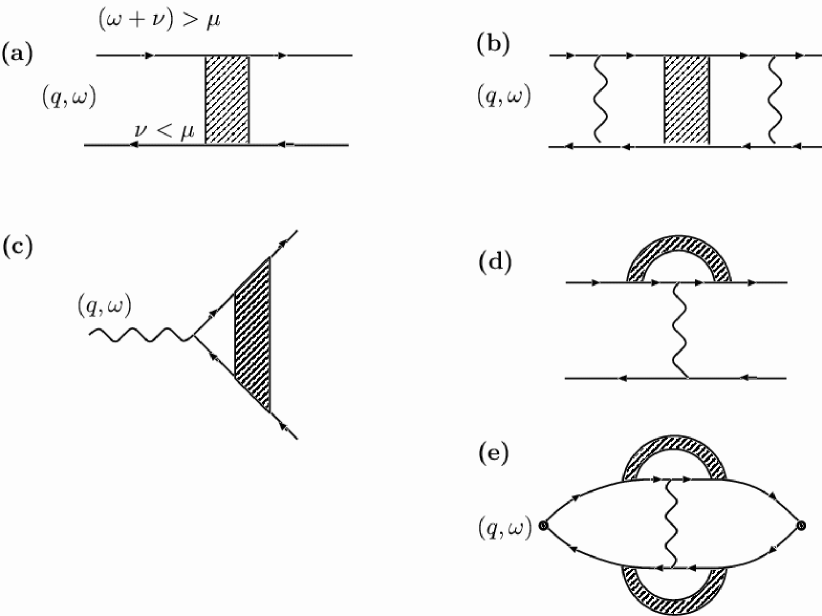
Figure 66: Elementary processes important in the problem of two-dimensional disordered interacting electrons and referred to in the text. (a) Representation of the diffusion propagator due to impurity scattering vertices and corresponding self-energy. The particle lines and hole lines should be on opposite sides of the chemical potential. (b) Singular second-order interactions. (c) Singular vertex in the density channel (and in the spin-density channel for the spin-conserving problem). (d) Singular (irreducible) first-order interactions. (e) Elementary singular polarization propagator.

The diffusive form of the density correlation function and spin-density correlation is the genesis of the singularities due to interactions in two-dimensions. For example the elementary effective vertex in Fig. 66 due to a bare frequency-independent short-range interactions in two-dimensions is

$$v^{2}\ \intop_{o}^{\ell^{-1}}\ dq~{}q\left({1\over i\omega+Dq^{2}}\right)\approx\ v^{2}\ N(0)~{}\ln(\omega\tau)\ \>.$$ (221)

The singularity arises because $\pi(\omega,q)=f(\omega/Dq^{2})$. Recall that for pure electrons $\pi(\omega,q)=f(\omega/v_{F}q)$ leading to a logarithmic singularity for the second-order vertex in one-dimension and regular behavior in higher dimensions. Similarly $\pi(\omega,q)=f(\omega/q^{3})$ leads to a logarithmic singularity in the second-order vertex in three-dimensions, as we saw in section 5.1 on SFL’s due to Gauge interactions.

Note that in Eq. (221) and other singular integrals in the problem have ultra-violet cutoffs at $q\approx\ell^{-1}$ and $\omega\approx\tau^{-1}$ since the diffusive form is not applicable at shorter length scales or time scales. It also follows that Boltzmann transport theory is valid at temperatures larger than $\tau^{-1}$.

Actually even the first order interaction dressed by diffusion fluctuations is singular. Consider first the diffusion correction to the vertex shown in Fig. 15

$${\Lambda\over\Lambda_{o}}\ =\ {1\over\tau}\ \left(i\omega\ +\ Dq^{2}\right)^{-1}\>,$$ (222)

provided $\epsilon<0,\epsilon-\omega>0$ or vice-versa. The restriction is a manifestation of point (3) and arises because in the diffusion process, only intermediate states with one line above (particle) and the other below (hole) the chemical potential contribute as they alone define the physical density. This leads to the first order irreducible interaction and the polarization graph shown in Fig. 67 to be logarithmically singular.

For the small $q$ of interest for singular properties, one need consider interactions only in the $s$-wave channel. One then has two interaction parameters, one in the singlet channel and the other in the triplet channel.

Consider the problem with Coulomb interactions. Then the effective interaction in the singlet channel sums the polarization bubbles connected by Coulomb interactions. Using (218) for the polarization bubble, it is shown [14] that for small momentum transfer the interaction in the spin singlet $(S=0)$ channel, Fig. 67, becomes

$$V_{\mbox{\footnotesize singlet}}=2\kappa~{}.$$ (223)

In the non-interacting limit $\kappa=N(0)$, independent of density. Consider now the ladder-type interactions illustrated in Fig. 68. These involve both the singlet and the triplet interactions. The momentum carried by the interaction lines is however to be integrated over. Therefore the triplet-interactions do not have a universal behavior, unlike the singlet interactions.

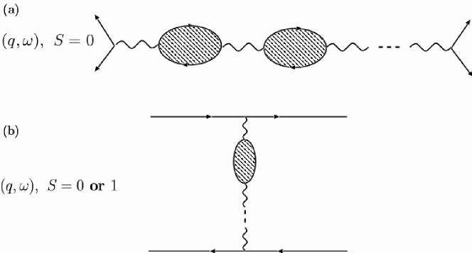
Figure 67: Effective interactions can be split up into singlet and triplet channels. In the singlet-only channel (a), the density-density interaction is screened by the Coulomb interaction and is universal at long wavelengths. In the triplet channel and in the singlet channel for large momentum, the screened density-density interaction appears only in the cross channel and is therefore non-universal.

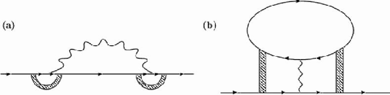
Figure 68: Simplest processes contributing to the singular self-energy. (a) Exchange process. (b) Hartree process.

Altshuler, Aronov and collaborators [14] calculated the logarithmic corrections to first-order in the interactions for various physical quantities. To these one can add the contribution already discussed due to weak-localization. The corrections to the single-particle density of states, the specific heat and the conductivity over the non-interacting values are respectively:

$${\delta N\over N}\ = {1\over 4\pi\epsilon_{F}\tau}\ \ln|\omega\tau|\left|\ln|{\omega\over\tau(Ds^{-2})^{2}}|\right|~{},$$ (224)

$${\delta C\over C}\ = \ {1\over\pi\epsilon_{F}\tau}\ \left(1-{3\over 2}F\right)\ln|T\tau|~{},$$ (225)

$${\delta\sigma\over\sigma}\ = \ {1\over 4\pi^{2}}\ \left(2-{3\over 2}F\right)\ln|T\tau|\>.$$ (226)

The compressibility has no logarithmic correction. In these equations, $s$ is the screening length and $F$ is a parameter which is of the order of the dimensionless interaction $r_{s}$.

The first terms in (225) and (226) are due to exchange processes and the second due to the Hartree processes. The exchange process, of which the contribution to the self-energy is shown in Fig. 66, use the interaction in the singlet channel; hence the universal coefficient. The second contribution uses both triplet and the (large $q$ part of the) singlet interactions. In first-order of interaction the difference in sign of the two processes is natural. In pure systems, the Hartree process does not appear as it involves the $q=0$ interaction alone which is exactly canceled by the positive background. For disordered systems, due to the fluctuation in the (ground state) density, a first order Hartree process, Fig. 68 contributes.

In the presence of a magnetic field the $S_{z}=\pm 1$ parts of the triplet interactions acquire a low-energy cut-off. Therefore the logarithmic correction to the resistivity is suppressed leading to negative magneto-resistance proportion to $F(H/kT)^{2}$ for small $H/kT$ but $g\mu_{B}H>>\tau^{-1}_{so},\tau^{-1}_{s}$ where $\tau^{-1}_{so}$ and $\tau^{-1}_{s}$ are spin-orbit and spin-scattering rates respectively, for appropriate impurities.

8.4 Finkelstein Theory

Finkelstein [90] has used field-theoretical methods to generalize Eqs. (224)-(226) beyond the Hartree-Fock approximation. His results have been rederived in customary diagrammatic theory [51, 39]. The interference processes leading to weak localization are again neglected. The theory may be regarded as first order in $1/k_{F}\ell$. In effect the method consists in replacing the parameter $F$ by a scattering amplitude $\gamma_{t}$ for which scaling equations are derived. The equivalent of the $F^{s}_{o}$ parameter is fixed by imposing that the compressibility remains unrenormalized, i.e., does not acquire logarithmic corrections. A second important quantity is a scaling variable $z$, which is analogous to the dynamical scaling exponent $z$ which we discussed in the section 6, which gives the relative scaling of temperature (or frequency) with respect to the length scale. A very unusual feature of the theory is that $z$ itself scales! Scaling equations are derived for $\gamma_{t}$ and $z$ to leading order $1/k_{F}\ell$. As $T\to 0$, both $\gamma_{t}$ and $z$ diverge. The divergence in $z$ (see the discussion in section 7) usually means that the the momentum dependence of the fluctuations is unimportant compared to their frequency dependence. The divergence in $\gamma_{t}$ as $T\rightarrow 0$ in such a case has been interpreted to imply divergent spatially localized magnetic-fluctuations; in other words, it implies the formation of local moments [91, 53]. At the same time, the scaling equations show conductivity flowing to a finite value.

The scaling trajectories of Finkelstein’s theory are shown schematically in Fig. 69. While in the non-interacting theory with disorder, one always has an insulator, this theory flows always towards a metal. However the theory cannot be trusted beyond $\gamma_{t}\sim 1$ beyond which it is uncontrolled. The theory also cannot be trusted for large disorder, $k_{F}\ell\sim{\mathcal{O}}(1)$ , even for small interactions.

It is worth emphasizing that Finkelstein’s theory gives an effect of the interactions in a direction opposite to the leading perturbative results. The perturbative results themselves of course are valid only for small $r_{s}$ while Finkelstein theory is strictly valid only for $r_{s}<{\mathcal{O}}(1)$. One possibility is that the Finkelstein result itself is a transient and the correct theory scales back towards an insulator. Another possibility is that it correctly indicates (at least for some range of $r_{s}$ and disorder) a strong-coupling singular Fermi-liquid metallic fixed line. The new experiments discussed below can be argued to point to the latter direction.

It is hard except in very simple situations (the Kondo-problem, for instance) to obtain the approach to a strong-coupling fixed point analytically. In that case one may usually guess the nature of the fixed point and make an expansion about it to ascertain its stability.

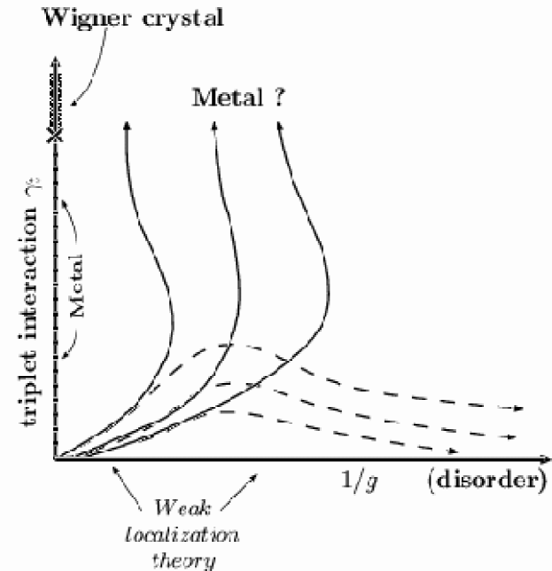
Figure 69: Schematic renormalization group flow for the disordered interacting electron problem according to the Finkelstein theory. dashed lines represent the effect on the solid lines on applying a magnetic- field which couples to spins alone.

In making such a guess, the SFL properties towards which the Finkelstein solution flows should be kept in mind:

(i) The conductivity flows towards a finite value in the theory as $T\rightarrow 0$.
(ii) The density of single-particle states flows towards zero

$$N(\omega)\sim\omega^{\alpha}~{}.$$ (227)

(iii) The magnetic susceptibility diverges at a finite length scale (the effect of a diverging $z$) indicating the formation of local moments.

The last point appears to be crucial. As may be seen from Eq. (234) below, the growth of the triplet scattering overrides the exchange processes which favor the insulating state. Indeed if the triplet divergence is suppressed by an applied magnetic field, the theory reverts to the perturbative form of Eq. (215). The scale of the magnetic-field for this effect is given by the temperature. The formation of localized regions of moments may be linked to the fact already discussed that the ferromagnetic state is close in energy to the paramagnetic fluid (and the crystalline states) as density is decreased. The experiments discussed below have a significant correspondence with this picture, although there are some crucial differences.

A possible strong coupling fixed point is a state in which the local moments form a singlet state with a finite spin stiffness of energy of ${\mathcal{O}}(H_{c})$. This eliminates any perturbative instability of the triplet channel about the fixed point. The state is assumed to have zero density of single-particle states at the chemical potential. This eliminates the localization singularity as well as well as the singularity due to the singlet channel. This state is then perturbatively stable. The issue of whether such a state has finite conductivity is unresolved. The occurrence of a new characteristic scale $H_{c}$ observed in the magneto-resistance experiments discussed below with $H_{c}\rightarrow 0$ as the metal-insulator transition in zero field as $n\rightarrow n_{c}$ is also in correspondence with these ideas.

8.5 Compressibility, Screening length and a Mechanism for Metal-Insulator Transition

Suppose the metallic state in two dimensions is described by a fixed point hinted by the Finkelstein theory and expansion about it. Such a description must break down near the critical $r_{s}$ where a first order transition to the Wigner transition must occur in the limit of zero disorder. General arguments suggest that the transition for finite disorder must be continuous [124].

A suggestion for the breakdown of the Finkelstein regime follows from the calculation of the correction to the compressibility due to disorder [226]. As already mentioned, no perturbative singularity is found in the compressibility due to interactions. However, the correlation energy contribution of the zero-point fluctuations of plasmons is altered due to disorder with a magnitude which depends also on $r_{s}$. The leading order contribution in powers of $(k_{F}\ell)^{-1}$ can be calculated for arbitrary $r_{s}$. Including this contribution the compressibility $\kappa$ may be written in the form

$$\frac{\kappa_{0}}{\kappa}=\frac{\kappa_{0}}{\kappa}_{pure}+0.11r_{s}^{3}/(\omega_{0}\tau)+{\mathcal{O}}\left((r_{s}^{4})/(\omega_{0}\tau)^{2}\right).$$ (228)

Here $\kappa_{pure}$ is the compressibility for zero disorder, $\kappa_{0}=N(0)$, and $\omega_{0}$ is the Rydberg. In the Hartree-Fock approximation

$$\frac{\kappa_{0}}{\kappa}_{pure}=1-(\sqrt{2}/\pi)r_{s}$$ (229)

The best available numerical calculations also give $\kappa_{0}/\kappa$ varying slowly enough with $r_{s}$ that the correction term (228) dominates for $r_{s}$ of interest near the metal-insulator transition even for modest disorder; for example for $\omega_{0}\tau\approx 10$, the disorder contribution in Eq. (228) is larger than the pure contribution for $r_{s}\geq 10$. This has an important bearing on the Metal-Insulator transition because the screening length $s$ is given by

$$s/s_{0}=\kappa_{0}/\kappa~{},$$ (230)

where $s_{0}=a_{0}/2$. Strictly speaking $s$ is the screening length for an external immobile charge and the screening of the electron-electron interactions is modified from (228) due to vertex renormalizations. But in this case they do not change the essential results. From Eq. (228) it follows that the screening length $s(\ell)>\ell$, the mean-free path, for

$$r_{s}\geq 3(\omega_{0}\tau)~{}.$$ (231)

Suppose the condition $s(\ell)>L>\ell$ is satisfied. Here L again is the size of the box for which the calculation is done, defined through $DL^{-2}\approx T$. The assumption of screened short-range interactions, with which perturbative corrections leading to results of Eqs. (224), (225), and (226) are obtained, is no longer valid. In this regime the calculations must be done with unscreened Coulomb interactions. The correction proportional to F in Eqs. (224), (225), and (226) is not modified but the singlet contributions are more singular (due to the extra $q^{-1}$ in the momentum integrals). For instance, Eq. (226) is modified to

$$\delta\sigma/\sigma=-(\sqrt{2}/\pi^{2})r_{s}\frac{L}{\ell}~{}.$$ (232)

This implies a crossover to strong localization. It is therefore suggested that the metallic state ceases to exist when condition (231) is satisfied.

The above line of reasoning is of particular interest because as discussed below a sharp variation in the compressibility is indeed observed to accompany the transition from the metallic-like to insulating-like state as density is decreased (as shown in Fig. 79 below).

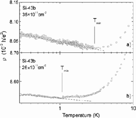
Figure 70: Resistivity data on a fine scale for the two highest densities in Fig. 75 below, showing correspondence with the theory of weak localization at such high densities. From Pudalov et al. [202].

8.6 Experiments

Soon after the publication of the theory of weak localization its predictions were seemingly verified in experiments on $Si$-MOSFETS [47, 245]. The experiments measured resistivity on not very clean samples of high density with resistivity of $O(10^{-2}h/e^{2})$. In a limited range of temperature the predicted logarithmic rise in resistivity with decreasing temperature with about the right prefactor was found [40]. In view of the perturbative results of Altshuler and Aronov [14] and the knowledge that electron-electron interactions alone lead to a Wigner insulator at low densities, one was led to the conviction that the metallic state does not exist in two dimensions. It was expected that samples will larger $r_{s}$ will simply show logarithmic corrections to the resistivity at a higher temperature and pure samples at a lower temperature. Not too much attention was paid to Finkelstein’s results which pointed to the more interesting possibility of corrections in the opposite direction.

Figure 71: Resisitivity as a function of temperature for a wide range of densities (and Fermi-energy) in a disordered $Si$ MOSFET. The inset shows accurate measurements of $\rho(T)$ close to the speparatrix for another sample. From Sarachik and Kravchenko [211, 3].

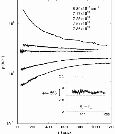
Figure 72: Resistivity versus temperature at five different electron densities in the experiments of Kravchenko and Klapwijk [142]. The inset shows that the middle curve ($n_{s}=7.25\times 10^{10}cm^{-2}$) changes by less than $\pm 5$% in the entire temperature range.

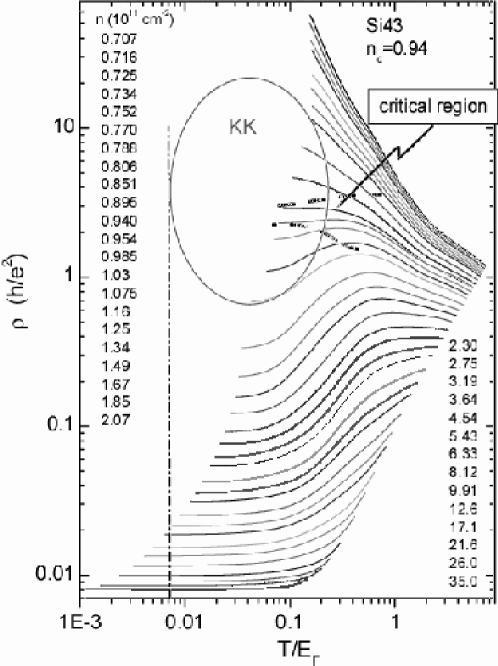
Figure 73: Plot of the resistivity as a function of the scaled temperature $T/E_{F}$. The encircled region indicates the range of parameters explored in Fig. 72 and in [142]. The dash-dotted vertical line depicts the empirical temperature $T_{Q}=0.007E_{F}$ below which the logarithmic temperature dependence like that of Fig. 70 sets in. From Prinz et al. [200].

The more recent experiments on a variety of samples on a wider range of density and of higher purity than earlier have re-focused attention on the problem of disorder and interactions in two dimensions and, by implication, in three dimensions as well. Several reviews of the experiments are available [3, 16, 17]. We will present only a few experimental data to highlight the theoretical problems posed, and will focus on the behavior of the data as function of temperature. The scaling of the data as a function of the electron density $n-n_{c}$ or field $E$ will not be discussed; there is a considerable body of data on nonlinear $E$-dependence (see e.g. [223] and references therein) but the significance of the data is not clear at present.

The first thing to note is that results consistent with the earlier data [47, 245] are indeed obtained for high enough densities. Fig. 70 shows the resistance versus temperature in $Si$ for $r_{s}\sim{\mathcal{O}}(1)$. The magnitude of the temperature dependence is consistent with the predictions of weak localization corrections. As we will show below in the same region of densities, the negative magneto-resistance predicted as correction to weak-localization, discussed above, is also observed.

Fig. 71 shows the resistivity as a function of $T$ over a wide range of densities. Similar data from [142] over a large small of densities is shown in Fig. 72, and data over a large range of densities are plotted as a function of $T/E_{F}$ in Fig. 73. The resistivity clearly shows a change of sign in the curvature as a function of density at low temperatures. The resistivity at the cross-over density as a function of temperature is shown down to 20mK in the inset to Fig. 72 and is consistent with temperature independence. The true electron temperature in these samples is a question of some controversy [16, 3], but more recent experiments, whose data are shown in Fig. 74, have corroborated these results by studying this issue very carefully down to 5mK. In the high density region the resistivity does rise with decreasing temperature logarithmically, consistent with earlier measurements. The consistency of these data sets for two very different types of samples therefore gives strong evidence that these are genuine effects in both types of systems.

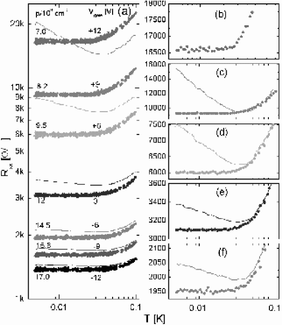
Figure 74: (a) Temperature dependence of the longitudinal resistivity of a 2D hole gas for various gate biases and associated densities in experiments on $GaAs$. The solid curves are estimated weak localization predictions. (b)-(f): Magnified view of the data in (a) averaged over a 5% temperature interval. The estimated weak localization prediction has been shifted to coincide with the data curve at $T=50mK$. From Mills et al. [172]

The data shown in Figs. 71-73 is for $Si$-MOSFET samples. The data for $GaAs$ heterostructures, and $Si$ in other geometries is qualitatively similar [115, 61, 62, 196, 114, 172]. Fig. 74 shows data on high quality gated GaAs quantum wells with densities on the metallic side of the metal-insulator ”transition” taken to temperatures as low as 5mK. The resistivity is essentially temperature independent at low temperatures; the logarithmic corrections expected from weak-localization (calculated using the measured resistivity and the theoretically expected $\tau_{\phi}$) is also shown.

Experiments in a Parallel Magnetic Field: A magnetic field applied parallel to the plane couples primarily to the spin of the electrons. For small-fields and for $n\gg n_{c}$, a positive magneto-resistance proportional to $H^{2}$ is observed as expected from perturbative calculations in the interactions. For fields such that $\mu_{B}H\approx E_{F}$, the electrons are fully polarized and the resistivity saturates as expected. The temperature dependence of the resistivity begins to be insulating-like at low temperatures with the cross-over temperature increasing as $n$ decreases [228]. This is an indication that the metallic state becomes unstable as the spins are polarized. A complete set of data is shown in Fig. 75 where resistivity versus temperature in a $Si$-MOSFET with density varying across $n_{c}$ is shown together with the resistivity versus magnetic-field at the lowest temperature for some densities on the $n>n_{c}$ side. It is noteworthy that the temperature dependence of the high-field data (not shown) appears to fall on the curve of resistivity versus temperature (at H=0) which the high field (low temperature) data saturates asymptotically.

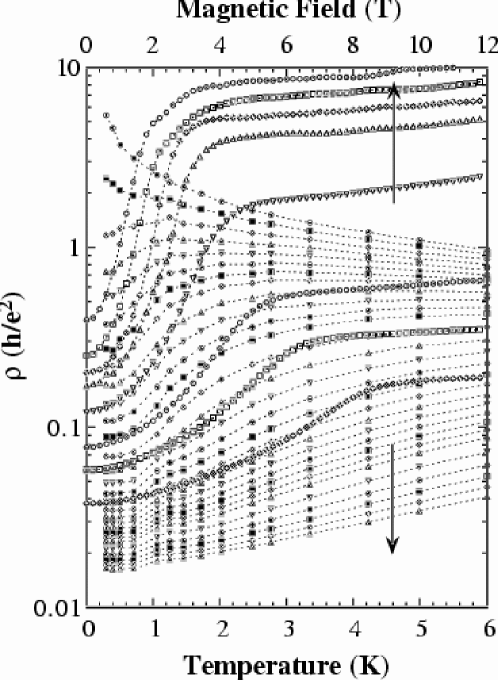
Figure 75: Results for resistivity versus temperature and versus magnetic field applied in the plane for a few densities on either side of $n_{c}$ . The magnetic field is shown on the upper axis and the data is taken at the lowest temperature for some of the densities shown in the resistivity versus temperature plots. From Pudalov et al. [201].

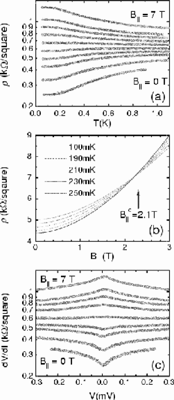
Figure 76: Plot of the magnetoresistance. In (a) the $T$ dependence of $\rho$ in the zero field metallic phase is shown on a semilog plot for a hole density $3.7\times 10^{10}cm^{-2}$ for varying $B_{||}$ values. As $B_{||}$ increases from zero, the strength of the metallic behavior measured by the total change in $\rho$ from about 1K to 50mK weakens progressively, and for $B_{||}\geq B_{c}$ $d\rho/dT$ becomes negative (i.e. the system becomes insulating). An alternate way of demonstrating the existence of a well defined $B_{||}^{c}$ is to plot $\rho$ against $B_{||}$ at several different temperatures. In (b)  $\rho$ is plotted vs $B_{||}$ at a hole density $1.5\times 10^{10}cm^{-2}$. $B_{||}^{c}$ is read off the crossing point marked by the arrow. In (c), the differential resistivity $dV/dI$ is measured at 50mK across the $B_{||}$ induced Metal-Insulator transition is shown at magnetic field strengths similar to those in (a). From Yoon et al. [279].

The parallel magneto-resistance has been examined carefully for $n$ close to but larger than $n_{c}$, and is shown in Figs. 76 for $p$-type $GaAs$ [279]. Qualitatively similar results are found in $n$-type $Si$ [203]. It is discovered that a critical field as a function of density $H_{c}(n)$ exists such that for $H<H_{c}(n)$ the resistivity continues to be metallic-like $d\rho/dT>0$ and for $H>H_{c}(n)$ it is insulating like $d\rho/dT<0$. The field $H_{c}(n)$ tends to zero as $n\rightarrow n_{c}$. The low temperature data on the high fields side is puzzling and should be re-examined to ensure that the electron-temperature is indeed the indicated temperature.

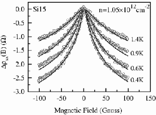
Figure 77: Plot of the magnetoresistance. The change in the resistivity $\Delta\rho(B)=\rho_{xx}(B)-\rho_{xx}(0)$ vs magnetic field $B$ at an electron density of 1.05 $\times$ 10¹² cm^-2 at various temperatures. The open circles denote the measurements and the full line is the best least square fit according to the single electron weak localization correction to the conductivity. From Brunthaler et al. [48].

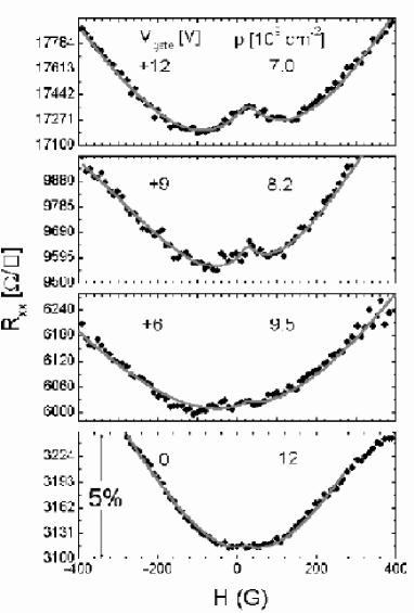
Figure 78: Variation of the longitudinal resistance with perpendicular magnetic field for 2D sample at $T=9mK$ and at various indicated densities. The weak-localization correction is estimated to be ${\mathcal{O}}(10^{2})$ larger than the observations at these densities. From Mills et al. [172].

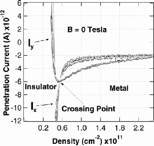
Figure 79: Compressibility data. In this experiment, at low frequencies, $I_{x}$ is directly proportional to $R_{x}$, the dissipation of the two dimensional hole system, while $I_{y}$ is proportional to the inverse compressibility. $I_{x}$ and $I_{y}$ are shown as a function of density for five different temperatures ranging from 0.33 K to 1.28 K at an excitation frequency of 100Hz. The crossing point of the five dissipation channel curves corresponds to the metal-insulator transition at $B=0$. The minimum of the inverse compressibility occurs at the same hole density of $5.5\times 10^{10}cm^{-2}$. From Dultz et al. [79].

Experiments in a Perpendicular Field: The behavior of a resistance in all but very small perpendicular fields, is dominated by the Quantum Hall Effect (QHE). The connection of the Quantum Hall transitions to the metal-insulator transition at $n=n_{c}$ and $H=0$ is an interesting question which we will not touch on. At low fields and for $n\geq n_{c}$, outside the QHE regime, negative magneto-resistance predicted by weak-localization theory are observed. Data for $n\gg n_{c}$ is shown in Fig. 77 and agrees quite well with the theoretical curves as shown; similar results for $n$ close to $n_{c}$ are also reported [114]. More recent low temperature data in $GaAs$ heterostructures[172] is reproduced in Fig. 78 for densities $n>n_{c}$ but close to $n_{c}$. A magnetoresistance two orders of magnitude smaller than the weak localization theory is estimated although the width of the negative magneto-resistance region is not in disaccord with the weak-localization correction.

Compressibility measurements Compressibility $(\kappa)$ measurements [79, 122] in the region around $n=n_{c}$ show a rapid change in $\kappa^{-1}$ from the negative value characteristic of high $r_{s}$ metallic state to positive values — see Fig. 79. These are very important measurements which show that a thermodynamic quantity has a very rapid variation near $n\approx n_{c}$. We have already discussed that such changes were predicted [226] to occur through perturbative corrections due to disorder to the energy of interacting electrons. Some more recent measurements [276] of the local electrostatic potential show that in the region $n\approx n_{c}$ large scale density fluctuations (puddles) occur with very weak connections between them. Completely isolated puddles evidently have $\kappa^{-1}=0$.

8.7 Discussion of the Experiments in light of the theory of Interacting Disordered Electrons

In comparing the experimental results with the theory, it is necessary to separate out the effects due to ”customary-physics” — for instance electron-phonon interactions, creation of ionized impurities with temperature [15], change of screening from its quantum to its classical form as a function of temperature [72] change of single particle wavefunctions with a magnetic fields [137], inter-valley scattering [277], etc. — from the singular effects due to impurities and interactions. The separation is at present a matter of some debate. However it seems that the following features of the experimental data in relation to the theoretical ideas summarized in sections 8.3, 8.4 are especially noteworthy. These must be read bearing in mind our earlier discussion that most of the interesting experiments are in a range of $r_{s}$ and disorder where the theoretical problems are unresolved and only hints about the correct form of a theory are available.

$\bullet$ At $r_{s}\leq{\mathcal{O}}(1)$ and $k_{F}\ell\gg 1$ a logarithmic increase in resistance with decreasing $T$ consistent with weak-localization as well as with the perturbative interaction correction is observed. A positive magneto-resistance consistent with the latter is also observed. Also observed is the correction to weak-localization due to phase-breaking of backscattering in a perpendicular magnetic field. The latter yields sensible values and temperature dependence for the phase relaxation rate given by the theory. It appears that at high enough density, the weak localization theory supplemented by the perturbative theory of interactions is in excellent agreement with the experiments in the range of temperatures examined.

$\bullet$ As $r_{s}$ is increased (and $k_{F}\ell$ decreased) the logarithmic resistance is lost in the observed temperature range, whereas weak-localization theory predicts that the coefficient of such terms (as well as the onset temperature for their occurrence) should increase. For $r_{s}$ not too large the decreased logarithmic term may be associated with the perturbative corrections (215) due to interactions.

$\bullet$ Upon further increasing $r_{s}$, the derivative $d\rho/dT$ becomes positive in the low temperature region as in a metal. The magneto-resistance in a parallel field is positive $\sim H^{2}$ as is predicted by Finkelstein [although the variation is closer to $H^{2}/T$ rather than as $(H/T)^{2}$] [203]. The phase breaking correction in a perpendicular field continues to be observed. But quite curiously the deduced $\tau_{\phi}$ is larger than $\tau$ deduced from resistivity — by definition a phase-breaking rate serves as a cutoff only if $\tau_{\phi}<\tau$.

$\bullet$ In the “metallic” regime for intermediate $r_{s}$, a strongly temperature dependent contribution for $T\leq E_{F}$ is found which may be fitted to the form $\rho^{\prime}(n)\exp(-E_{a}(n)/T)$. The magnitude of this term rapidly decreases as the density $n$ decreases. No accepted explanation for this contribution has been given. In $Si$ the change of resistivity at $n\approx 10n_{c}$ due to this contribution is an order of magnitude larger than in $GaAs$. It has been proposed [14, 201] that this contribution together with the weak-localization contribution may well account for all the data in the “metallic” regime since it pushes the minimum of the resistivity below which the logarithmic temperature dependence is visible to lower temperature than the available data at lower densities.

This issue can be resolved by experiments at lower temperatures. At this point, especially in view of the consistency of the recent results of Mills et al. — see Figs. 74 and 78 — with the earlier experiments, one can say that it requires an unlikely conspirancy of contributions to remove the temperature dependence over a wide range for different materials and with different degrees of disorder.

A quite different scenario also consistent with the existing data is that the logarithmic upturn in the resistivity observed in high density samples is a transient that on further decreasing the temperature disappears to be replaced by $\frac{d\rho}{dT}\rightarrow 0$ as $T\rightarrow 0$, at least above some characterestic density which is a function of diorder. We will come back to this issue when we discuss the possible phase-diagram.

$\bullet$ As $r_{s}$ approaches $r_{sc}$, $d\rho/dT$ tends to zero (through positive values). A separatrix is observed with $d\rho/dT\approx 0$ over about 2 orders of magnitude in temperature for $Si$ and over an order of magnitude in $GaAs$. For $r_{s}>r_{sc}$, $d\rho/dT$ is negative befitting an insulator. $r_{sc}$ appears to be smaller for dirtier samples but not enough systematic data is available for drawing a functional relation.

$\bullet$ The electronic compressibility rapidly changes near the ”transition” and rapidly becomes small on the insulating side. Its value on the insulating side is consistent with approaching zero in the limit of zero temperature. Although this is in qualitative accord with the theoretical suggestion [226], further experiments measuring simultaneously the compressibility and the conductivity at low temperatures are necessary to correlate the metal-insulator transition with the rapid variation of compressibility or the screening length. Note that it follows from the Einstein relation $\sigma=D\kappa$ that if $\kappa$ is finite in the metallic state ($\sigma$ finite) and zero in the insulating state ($\sigma=0$), $\kappa$ must go to zero at the transition. Otherwise we would have the absurd conclusion that $D\rightarrow\infty$ at the transition.

Interesting phenomenological connections between the transport properties and formation of ”puddles of electron density” of decreasing size as the metal-insulator ”transition’ is approached have been drawn [166].

$\bullet$ Near $r_{s}=r_{sc}$ the resistivity as a function of temperature on the insulating side appears to be a reflection of that on the metallic side about the $d\rho/dT=0$ line if the data is not considered to low temperatures [141]. Now with more complete data, we know that the resistivity flattens to zero slope at low temperatures on the ”metallic” side of $n_{c}$ . The most likely behavior appears to be that the resistivity approaches a finite value at low temperature on one side of $n_{c}$ and an infinite value on the other. A one-parameter scaling ansatz [75] for the problem with interaction and disorder gave $\rho\rightarrow\infty$ for $n<n_{c}$ and $\rho\rightarrow 0$ for $n>n_{c}$ as $T\rightarrow 0$ and reflection symmetry just as at any second-order transition with one scaling parameter. Does this necessarily imply that multi-dimensional scaling is required near this transition? But another important point to bear in mind is that since resistance does not depend on a length scale in two-dimensions, it need not be a function, in particular, of the correlation length near the transition. The resistivity is allowed to be finite on one side of a metal-insulator transition and infinite on the other even though the transition may be continuous and the correlation length diverges on either side with the same exponent. The glassy nature (Coulomb glass) of the insulating state is also expected to change the critical properties.

$\bullet$ The resisitivity at low temperatures for $n\ll n_{c}$ has been fitted to an activated form $\propto\exp(\Delta/T)^{\alpha}$ with $\alpha\approx 1/2$ and with $\Delta\rightarrow 0$ as $n\rightarrow n_{c}$. This is characteristic of a Coulomb glass [224]. Whether this is indeed the asymptotic low temperature form is not completely settled.

$\bullet$ The resistance at $n\approx n_{c}$ appears to vary from sample to sample but is within a factor of 3 of the quantum of resistance. It is worth emphasizing that $n_{c}$ is close to the density expected for Wigner crystallization. With Coulomb interactions and disorder, the insulating state is indeed expected to be Wigner glass. In that case one might expect singular frequency dependent properties and hysteretic behavior near the transition.

$\bullet$ For $r_{s}\approx r_{sc}$ the resistance in a parallel-field is especially noteworthy. In a parallel field $d\rho/dT$ decreases untill at a field $H=H_{c}(n)$ it changes sign. $H_{c}$ vanishes at $n_{c}$, the density where $d\rho/dT=0$ for $H_{\parallel}=0$. In this regime, $\rho(H,T,n)$ can be scaled as [279]

$$\rho\left(\frac{(n-n_{c})}{T^{\alpha}},\>\frac{(H-H_{c}(n-n_{c}))}{T^{\beta}}\right)$$ (233)

This means that the transition from the metallic state to the insulating state can be driven by a magnetic field. It appears that the ”metallic” state owes its existence to low-energy magnetic fluctuations which are quenched by a magnetic field. This is in line with Finkelstein theory and the flow diagram of Fig. 69 yet the existence of a scale $H_{c}$ is not anticipated by the calculations of Finkelstein (nor, of course, is the mere existence of $n_{c}$). As $H_{\parallel}$ is further increased $d\rho/dT$ approaches the insulating behavior characteristic of $n>n_{c}$ at $H_{\parallel}=0$. At a fixed temperature the resistivity saturates for $g\mu_{B}H_{\parallel}\geq E_{F}$, i.e. for a fully polarized band.

For small perpendicular fields, negative magneto-resistance of the form of (215) continues to be observed at least for $Si$ for $n\gg n_{c}$. In $GaAs$ this contribution at least in the range $n_{c}\geq n\geq 2n_{c}$ is negligible.

$\bullet$ The Hall coefficient $R_{H}$ is continuous across the transition, obeying the kinetic theory result $R_{H}\sim 1/n$. On the “metallic” side this is not surprising. On the “insulating” side this is reminiscent of the properties of Wigner glasses [60, 105]

8.8 Phase Diagram and Concluding Remarks

It is worthwhile to try to guess the $T=0$ phase-diagram of interacting disordered electrons on the basis of the data and the available theory, inadequate though it is. A convenient set of axes is $r_{s}$ (or $n^{-1/2}$), as it parameterizes the dimensionless interaction, and the resistance in units of $h/e^{2}$ as it parametrizes the dimensionless disorder, see Fig. 80.

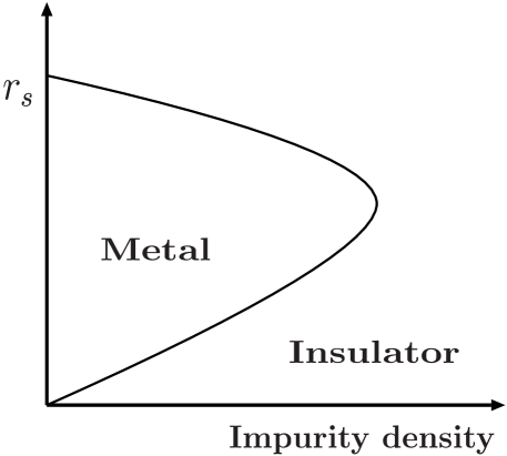
Figure 80: A tentative phase diagram at $T=0$ for two-dimensional disordered electrons with interactions.

Reliable theoretical results are found only along the two axes of Fig. 80. States are localized all along the horizontal axis. Localized states at $T=0$ must be organized into one or another kind of magnetically ordered state. On the vertical axis a Fermi-liquid gives way via a first order transition to a Wigner crystal which may have various magnetic phases.

In light of the experiments, the assumption made too long that the entire region in Fig. 80 is an insulator has to be abandoned in all likelihood. There does appear to be a ”metallic state”. With disorder a crossover to a Wigner glass must occur at large $r_{s}$. It is also clear that at high densities weak-localization theory supplemented by perturbative corrections due to interactions works quite well in the range of temperatures examined. At moderate $r_{s}$ for small disorder the Finkelstein correction appears to take over and a “metallic” state takes over. The best evidence for this, paradoxically, is the magnetic filed (parallel to the plane) dependence of the resistivity which appears to eliminate the “metallic” state.

Based on these considerations, the phase diagram Fig. 80 is put forth. It is surmised that the weak localization correction flows to strong localization for sufficiently strong disorder and small enough $r_{s}$, but that it gives way to a metallic state at weak-disorder and larger $r_{s}$. What determines the boundary? A possible criterion is that on one side the Finkelstein renormalization is more important and on the other side localization due to disorder is more important. The cross-over to strong localization occurs at a length scale $\zeta$ given by Eq. (209) where the resistivity doubles.

The scaling equation for the triplet interaction parameter is [90, 50, 149]

$$d\gamma_{t}/d\ln L=\ \pi\ k_{F}\ell\left(1+2\gamma_{t}\right)^{2}~{},$$ (234)

so that for small initial value $\gamma_{t}^{o}$ at $L=\ell$ one gets $\gamma_{t}(L)=\gamma_{t}^{o}+(\pi k_{F}\ell)\ln(L/\gamma)$. As $L=\zeta$, $\gamma_{t}\approx\gamma_{t}^{o}+1$. The boundary between the “metallic” and the “insulating” regions on this basis is linear at small $r_{s}$ and small $g^{-1}$, as shown in Fig. 80. This is highly conjectural but the existence of the phase boundary at the point $r_{s}\rightarrow 0$ and $1/g\rightarrow 0$ is more robust.

This scenario can be tested in high density, low disorder samples by measurements of resistivity at very low temperatures. If correct in some regime of parameters near the boundary, the logarithmic weak-localization correction should appear at high temperatures and disappear at lower temperatures.

We have stressed that the “metallic state” in 2-dimensions is likely to be a Singular Fermi-liquid with an interesting magnetic-ground state. Direct or indirect measurements of the magnetic susceptibility through, for instance the magnetic field dependence of the compressibility should yield very interesting results. Also interesting would be measurements of the single-particle density of states through tunneling measurements. Further systematic and careful measurements of the compressibility are also required to correlate the transition from the “metallic” state to the increase in susceptibility.

The basic theoretical and experimental problem remains the characterization of the “metallic state” its low temperature entropy,magnetic susceptibility, single-particle density of states etc. The experimental and theoretical problems are many but one hopes not insurmountable.

9 Acknowledgements

This article is an outgrowth of lectures delivered in spring 2000 by C. M. Varma during his tenure as Lorentz Professor at the Universiteit Leiden. He wishes to thank the faculty and staff of the Physics department and the deep interest shown by the attendees of the lectures.

Special thanks are due to numerous colleagues who provided the experimental data and who explained their ideas and clarified countless issues.

ZN also wishes to take this opportunity to greatly thank his former mentor, S. A. Kivelson, for coaching in one-dimensional physics.

Finally, ZN and WvS also wish to express their thanks to Debabrata Panja, Michael Patra, Kees Storm and especially Carlo Beenakker from the Instituut-Lorentz for all their help in generating, scanning, and compressing the numerous figures.

References

- [1] E. Abrahams, P. W. Anderson, D.C. Licciardo and T. V. Ramakrishnan, Scaling Theory of Localization: Absence of Quantum Diffusion in Two Dimensions, Phys. Rev. Lett. 42, 673 (1979).
- [2] E. Abrahams and C. M. Varma, What angle-resolved photoemission experiments tell about the microscopic theory for high-temperature superconductors, Proc. Nat. Academy of Sciences, 97, 5714 (2000).
- [3] E. Abrahams, S. V. Kravchenko and M. P. Sarachik, Metallic Behavior and Related Phenomena in Two Dimensions, cond-mat/0006055 (to appear in Rev. Mod. Phys.).
- [4] A. A. Abrikosov, L. P. Gorkov and I. Dzialoshinsky, Methods of Quantum field Theory in Statistical Physics, (Prentice-Hall, New Jersey, 1963).
- [5] See, e.g., A. A. Abrikosov, Fundamentals of the Theory of Metals (North-Holland, Amsterdam, 1988).
- [6] I. Affleck, T. Kennedy, E. H. Lieb, and H. Tasaki, Rigorous results on valence-bond ground states in antiferromagnets, Phys. Rev. Lett. 59, 799 (1987).
- [7] I. Affleck, A. W. W. Ludwig, H.-B. Pang and D. L. Cox, Relevance of anisotropy in the multichannel Kondo effect: Comparison of conformal field theory and numerical renormalization-group results, Phys. Rev. B 45, 7918 (1992).
- [8] I. Affleck and A. W. W. Ludwig, Exact critical theory of the two-impurity Kondo model, Phys. Rev. Lett.68, 1046(1992).
- [9] I. Affleck, A. W. Ludwig and B. A. Jones, Conformal-field-theory approach to the two-impurity Kondo problem: Comnparison with numerical renormalization-group results, Phys. Rev. B 52, 9528 (1995).
- [10] H Alloul Comment on “Nature of the conduction-band states in YBa2Cu3O7 as revealed by its Yttrium Knight shift”, Phys. Rev. Lett. 63, 689 (1989).
- [11] B. L. Altshuler, A. G. Aronov and P. A. Lee, Interaction Effects in Disordered Fermi Systems in Two Dimensions, Phys. Rev. Lett 44 ,1288 (1980).
- [12] B. L. Altshuler, A. G. Aronov and D. E. Khmelnitskii, Suppression of Localization Effects by the High Frequency Field and the Nyquist Noise, Solid State Commun. 39, 619 (1981).
- [13] B. L. Altshuler, A. G. Aronov and D. E. Khmelnitskii, Effects of electron-electron collisions with small energy transfers on quantum localization, J. Phys. C 15, 7367 (1982).
- [14] B. L. Altshuler and A. G. Aronov, in Eletron-Electron Interactions in Disordered Systems edited by A. L. Efros and M. Pollak, Elsevier, Science Publishers, New York (1985).
- [15] B. L. Altshuler and D. L. Maslov, Theory of Metal-Insulator Transitions in Gated Semiconductors, Phys. Rev. Lett. 82, 145 (1999).
- [16] B. L. Altshuler, D. L. Maslov and V. M. Pudalov, Metal-insulator transtion in 2D: resistance in the crititcal region, cond-mat/0003032.
- [17] B. L. Altshuler, G. W. Martin, D. L. Maslov, V. M. Pudalov, A. Prinz, G. Brunthaler, and G. Bauer, Weak-localization type description of condution in the “anomalous” metallic state, cond-mat/0008005.
- [18] P. W. Anderson, Absence of Diffusion in certain Random Lattices, Phys. Rev. 109, 1492 (1958).
- [19] P. W. Anderson, Localized Magnetic States in Metals, Phys. Rev. 124, 41 (1961).
- [20] P. W. Anderson, Infrared Catastrophe in Fermi gases with local scattering potential, Phys. Rev. Lett. 18, 1049 (1967).
- [21] P. W. Anderson, A Poor Man’s Derivation of Scaling Laws for the Kondo Problem, J. Phys. C 3, 2436-2441 (1970).
- [22] P. W. Anderson and G. Yuval, Exact results in the Kondo problem: equivalence to a classical one-dimensional Coulomb gas, Phys. Rev. Lett. 23, 89 (1969).
- [23] P. W. Anderson, G. Yuval, and D. R. Hamann, Exact Results in the Kondo Problem II. Scaling Theory, Qualitatively Correct Soution, and Some new Results on One-Dimensional Classical Statistical Models, Phys. Rev. B 1, 4464 (1970).
- [24] P. W. Anderson, The Theory of Superconductivity in the High Cuprates, (Princeton University Press, Princeton, 1997).
- [25] P. W. Anderson, Mat. Res. Bull. 8, 153 (1973)
- [26] T. Ando, A. B. Fowler, and F. Stern, Electronic properties of two-dimensional systems, Rev. Mod. Phys. 54, 437 (1982).
- [27] B. Andraka and A. M. Tsvelik, Observation of non-Fermi-liquid behavior in , Phys. Rev. Lett. 67 2886 (1991).
- [28] K. Andres, J. E. Graebner, and H. R. Ott, 4f-virtual-bound-state formation in at low temperatures, Phys. Rev. Lett. 35, 1779 (1975).
- [29] M. C. Aronson, M. B. Maple, R. Chau, A. Georges, A. M. Tsvelik and R. Osborn, Non-Fermi-Liquid scaling in (x=1, 1.5), J. Phys. Condens. Matter 8 9815 (1996).
- [30] M. C. Aronson, M. B. Maple, P. de Sa, R. Chau, A. M. Tsvelik and R. Osborn, Non-Fermi-Liquid scaling in (x=1, 1.5), A phenomenological description, Europhys. Lett. 46, 245 (1997).
- [31] O. M. Auslaender, A. Yacoby, R. de Picciotto, L. N. Pfeiffer and K. W. West, Experimental Evidence for Resonant-Tunneling in a Luttinger-Liquid, Phys. Rev. Lett. 84, 1756 (2000).
- [32] L. Balents and M. P. A. Fisher, Weak-coupling phase diagram of two-chain Hubbard model, Phys. Rev. B 53, 12133 (1996).
- [33] L. Balents and C. M. Varma, Ferromagnetism in Doped Excitonic Insulators, Phys. Rev. Lett. 84, 1264 (2000).
- [34] B. Batlogg and C. M. Varma, The underdoped phase of cuprate superconductors Physics World, 13, page 33 February 2000.
- [35] V. Barzykin and L. P. Gorkov, Ferromagnetism and Superstructure in , Phys. Rev. Lett. 84, 2207 (2000).
- [36] G. Baym and C. Pethick, Landau Fermi Liquid Theory, (Wiley, New York, 1991).
- [37] M. T. Béal-Monod and K. Maki, Renormalizability of Paramagnon Theories, Phys. Rev. Lett. 34 1461 (1975).
- [38] K. S. Bedell, Ed. Strongly Correlated Electronic Materials (Addison Wesley, New York, 1989).
- [39] D. Belitz and T. R. Kirkpatrick, The Anderson-Mott Transition, Rev. Mod. Phys. 66, 261 (1994).
- [40] G. Bergmann, Weak Localization in Thin Films Phys. Rep. 107, 1 (1984).
- [41] O. O. Bernal, D. E. MacLaughlin, H. G. Lukefahr, and B. Andraka, Copper NMR and thermodynamics of : Evidence for Kondo disorder, Phys. Rev. Lett. 75, 2023 (1995).
- [42] O. Betbeder-Matibet and P. Nozières, Transport Equation for Quasiparticles in a System of Interacting Fermions Colliding on Dilute Impurities, Ann. Phys. (N.Y.) 37 17 (1966).
- [43] B. Bogenberger and H. von Löhneysen, Tuning of non-Fermi-liquid behavior with pressure, Phys. Rev. Lett. 74, 1016 (1995).
- [44] N. Bogolubov,On the Theory of Superfluidity, J. Phys. USSR, XI, 23 (1947).
- [45] B. Bucher, P. Steiner, J. Karpinski, E. Kaldis, and P. Wachter, Influence of the SPin Gap on the Normal State Transport in YBa2Cu4O8 Phys. Rev. Lett. 70, 2012 (1993).
- [46] B. Bernu, L. Candido, D. M Ceperley, Exchange frequencies in the 2d Wigner crystal, cond-mat/0008062.
- [47] D. J. Bishop, D. C. Tsui, and R. C. Dynes, Nonmetallic Conduction in Electron Inversion Layers at Low Temperatures, Phys. Rev. Lett. 44, 1153 (1980).
- [48] G. Brunthaler, A. Prinz, G. Bauer, V. M. Pudalov, E. M. Dizhur, J. Jaroszynski, P. Glod, and T. Dietl Weak localization in the 2D metallic regime of Si-MOS, Ann. Phys. (Leipzig) 8, 579 (1999) [cond-mat/9911011].
- [49] H. Castella and X. Zotos, Exact calculation of spectral properties of a particle interacting with a one dimensional fermionic system, Phys. Rev. 47, 16186 (1993).
- [50] C. Castellani, C. Di Castro and W. Metzner, Dimensional crossover from Fermi to Luttinger Liquid, Phys. Rev. Lett. 72, 316 (1994).
- [51] C. Castellani, C. Di Castro, P. A. Lee and M. Ma, Interaction-driven metal-insulator transitions in disordered fermion systems, Phys. Rev. B 30, 527 (1984).
- [52] C. Castellani, C. Di Castro, G. Forgacs, and E. Tabet, Towards a Microscopic Theory of the Metal-Insulator Transition, Nuclear Phys. B 225, 441 (1983).
- [53] C. Castellani, C. Di Castro, P. A. Lee, M. Ma, S. Sorella, and E. Tabet Spin fluctuations in disordered interacting electrons Phys. Rev. B 30, 1596 (1984).
- [54] A. H. Castro Neto, G. Castilla, and B. A. Jones, Non-Fermi Liquid Behavior and Griffiths Phase in f-Elecron Compounds, Phys. Rev. Lett. 81 3531 (1998).
- [55] S. Chakravary, B. I. Halperin and D. Nelson, Low temperature behavior of two-dimensional quantum antiferromagnets, Phys. Rev. B 39, 2344 (1989).
- [56] S. Chakravarty, S. Kivelson, C. Nayak, and K. Voelker, Wigner glass, spin liquids, and the Metal-Insulator Transition, Phil Mag. B 79, 859 (1999).
- [57] S. Chakravarty, R. B. Laughlin, D. K. Morr, and C. Nayak, Hidden Order in the Cuprates, cond-mat/0005443.
- [58] S-W. Cheong, H. Y. Hwang, C. H. Chen, B. Batlog, L. W. Rupp, Jr., and S. A. Carter Charge-ordered states in for hole concentrations and 1/2, Phys. Rev. B 49, 7088 (1994).
- [59] Y. H. Chen, F. Wilczek, E. Witten, and B. I. Halperin, Int. J. Mod. Phys. B 3 1001 (1989).
- [60] P. Chitra, T. Giamarchi, and P. Le Doussal, Dynamical Properties of the pinned Wigner Crystal, Phys. Rev. Lett. 80, 3827 (1998).
- [61] P. T. Coleridge, R. L. Williams, Y. Feng, and P. Zawadzki, Metal-insulator transition at in p-type , Phys. Rev. B 56, R12764 (1997).
- [62] P. T. Coleridge, A. S. Sachrajda, and P. Zawadski, Weak localisation, interaction effects and the metallic phase of , cond-mat/9912041.
- [63] P. G. Collins and P. Avouris Nanotubes for Electronics Sci. Am., Dec. 2000, 38.
- [64] M. Combescot and P. Nozières, Infrared Catastrophy and Excitations in the X-ray Spectra of Metals, J. de Physique, 32, 913 (1971).
- [65] M. A. Continentino, Universal behavior in heavy fermions, Phys. Rev. B 47, 11587 (1993).
- [66] M. A. Continento, Quantum Scaling in Many Body Systems, Phys. Rep. 239, 179 (1994).
- [67] J. Corson and J. Orenstein, Normal State Conductivity Varies as Fractional Power of Transport Lifetime in a Cuprate Superconductor, cond-mat/0006027.
- [68] D. L. Cox, Quadrupolar Kondo effect in uranium heavy-electron materials?, Phys. Rev. Lett. 59, 1240 (1993).
- [69] D. L. Cox and M. Jarrell, The two-channel Kondo route to non-Fermi-liquid metals, J. Phys. Cond. Matt. 8, 9825 (1996).
- [70] D. L. Cox and A. Zawadowski, Exotic Kondo effects in Metals: magnetic ion in a crystalline electric field and tunneling centers, Adv. Phys. 47, 599 (1999).
- [71] S. Das Sarma and A. Pinczuk, Eds., Perspectives in Quantum Hall Effects, (Wiley, New York, 1997).
- [72] S. Das Sarma and E. H. Hwang, Charged Impurity-Scattering-Limited Low-Temperature Resistivity of Low-Density Silicon Inversion Layers, Phys. Rev. Lett. 83, 164 (1999).
- [73] C. Dekker, Carbon nanotubes as molecular quantum wires Phys. Today 52, 22 (1999).
- [74] A. de Visser, M. J. Graf, P. Estrela, A. Amato, C. Baines, D. Andreica, F. N. Gygax, and A. Schenck, Magnetic Quantum Critical Point in doped with , Phys. Rev. Lett. 85, 3005 (2000).
- [75] V. Dobrosavljević, E. Abrahams, E. Miranda, and S. Chakravarty, Scaling Theory of Two-Dimensional Metal-Insulator Transitions, Phys. Rev. Lett. 79, 455 (1997).
- [76] S. Doniach, The Kondo Lattice and Weak Antiferromagnetism, Physica B 91, 231 (1977).
- [77] S. Doniach and S. Englesberg, Low-Temperature properties of nearly ferromagnetic Fermi liquids, Phys. Rev. Lett. 17, 750 (1966).
- [78] S. Doniach and E. H. Sondheimer, Green’s functions for Solid State Physicists (Benjamin/Cummings, London, 1974).
- [79] S. C. Dultz, and H. W. Jiang, Thermodynamic Signature of a Two-Dimensional Metal-Insulator Transition, Phys. Rev. Lett. 84, 4689 (2000).
- [80] I.Dzyaloshinskii, A.M.Polyakov and P.wiegmann, Phys.letters,127A,112 (1988).
- [81] V. J. Emery, in Low-Dimensional Conductors and Superconductors, D. Jérome and L. G. Larson, eds. (Plenum, New York, 1987), p. 47.
- [82] V. J. Emery, in Highly Conducting One-Dimensional Solids, J. T. Devreese, R. P. Evrard and V. E. van Doren, eds. (Plenum, New York, 1979), p 247.
- [83] V. J. Emery and S. Kivelson, Mapping of the two-channel Kondo Problem to a resonant-level model, Phys. Rev. B 46, 10812 (1992).
- [84] V. J. Emery and S. Kivelson, Frustrated electronic phase separation and high temperature superconductors, Physica C 209, 597 (1993).
- [85] H. J. Eskes, R. Grimberg, W. van Saarloos, and J. Zaanen, Quantizing Charged Magnetic Domain Walls: Strings on a Lattice, Phys. Rev. B 54, R724 (1996).
- [86] P. Estrela, Non-fermi Liquid Behavior in Uranium based heavy-Fermion compounds, Thesis, University of Amsterdam (2000).
- [87] P. Estrela, L. C. J. Pereira, A. de Visser, F. R. de Boer, M. Almeida, M. Godinho, J. Rebizant, and J. C. Spirlet, Structural, magnetic and transport properties of single-crystalline , J. Phys. Cond Mat. 10, 9465 (1998).
- [88] M. Fabrizio, Role of transverse hopping in a two-coupled-chains model, Phys. Rev. B 48, 15838 (1993).
- [89] A. Fetter, C. Hanna, and R. B. Laughlin, The Random Phase approximation in the fractional-statistics gas, Phys. Rev. B. 39, 9679 (1998).
- [90] A. M. Finkel’stein, Influence of Coulomb interaction on the properties of disordered metals, Zh. Eksp. Teor. Fiz, 84, 168 (1983) [Sov. Phys. JETP 57, 97 (1983)].
- [91] A. M. Finkel’stein, Weak Localization and Coulomb Interaction in Disordered Systems, Z. Physik 56, 189 (1984).
- [92] A. I. Finkelstein, Soviet Scientific Reviews, page 3 (1990).
- [93] A. I. Finkelstein and A. I. Larkin, Two coupled chains with Tomonaga-Luttinger interactions, Phys. Rev. B 47, 10461 (1993).
- [94] J.O.Fjaerstad, A. Sudbo and A.Luther,Correlation functions for a two-dimensional electron system with bosonic interactions and a square Fermi surface, con-mat/9908296.
- [95] See M. E. Fisher, in Critical Phenomena, vol. 186 in Lecture Notes in Physics, F. J. W. Hahne, Ed. (Springer, Berlin, 1983).
- [96] M. P. A. Fisher and L. I. Glazman, Transport in a one-dimensional Luttinger liquid, in: “Mesoscopic Electron Transport”, L. Kouwenhoven, G. Schön and L. Sohn, eds., NATO ASI Series E (Kluwer, Dordrecht, 1997).
- [97] L. Forro, R. Gaál, H. Berger, P. Fazekas, K. Penc, I. Készmárki, and G. Mihály, Pressure Induced Quantum Critical Point and Non-Fermi-Liquid Behavior in , Phys. Rev. Lett. 85, 1938 (2000).
- [98] M. Fowler and A. Zawadowski, Scaling and the Renormalization Group in the Kondo Effect, Solid State Comm. 9, 471 (1971).
- [99] H. Fukuyama, Effects of Mutual Interactions in Weakly Localized Regime of Disordered Two-Dimensional Systems. II. Intervalley Impurity Scattering, J. Phys. Soc. Japan, 50, 3562 (1981).
- [100] Galitski, The Energy Spectrum Of a Non-Ideal Fermi Gas, Sov. Phys. JETP 7, 104 (1958).
- [101] A. Georges, G. Kotliar, W. Krauth, and M. J. Rozenberg, Dynamical mean-field theory of strongly correlated fermion systems and the limit of infinite dimensions, Rev. Mod. Phys. 68, 13 (1996).
- [102] T. Giamarchi and A. J. Millis, Conductivity of a Luttinger Liquid, Phys Rev. B 46, 9325 (1992).
- [103] T. Giamarchi, C. M. Varma, A. E. Ruckenstein, P. Nozières, Singular low-energy properties of an impurity model with finite range interactions, Phys. Rev. Lett. 70, 3967 (1993).
- [104] T. Giamarchi and H. J. Schulz, Anderson localization and interactions in one dimensional metals, Phys. Rev. B 37, 325 (1988).
- [105] T. Giamarchi and P. Le Doussal, Phase diagrams of flux lattices with disorder, Phys. Rev. B 55 6577 (1997).
- [106] Physical Properties of High Temperature Superconductors, Ed. D. M. Ginsberg (World Scientific, Singapore), Vol. I (1989), Vol. II (1990), Vol. III (1992), Vol. IV (1994).
- [107] S. M. Girvin, The Quantum Hall Effect: Novel Excitation and Broken symmetries, cond-mat/9907002.
- [108] H. R. Glyde, Excitations in liquid and solid Helium (Clarendon, Oxford, 1994).
- [109] A. O. Gogolin, A. A. Nersesyan, and A. M. Tsvelik, Bosonization and Strongly correlated Systems (Cambridge University Press, Cambridge, 1998).
- [110] M. Grayson, D. C. Tsui, L. N. Pfeiffer, K. W. West, and A. M. Chang, Continuum of Chiral Luttinger Liquids at the Fractional Quantum Hall Edge, Phys. Rev. Lett. 80, 1062 (1998).
- [111] F. M. Grosche, C. Pfleiderer, G. J. McMullan, G. G. Lonzarich, and N. R. Bernhoeft, Critical behaviour of , Physica B 206-207, 20 (1995).
- [112] B. I. Halperin and P. C. Hohenberg, Theory of dynamic critical phenomena, Rev. Mod. Phys. 49, 435 (1977).
- [113] B. I. Halperin, P. A. Lee and N. Read, Theory of the half-filled Landau level, Phys. Rev. B 47, 7312 (1993).
- [114] A. R. Hamilton, M. Y. Simmons, M. Pepper, E. H. Linfeld, P. D. Rose, and D. A. Ritchie, Reentrant Insulator-Metal Transition at in a Two-Dimensional Hole Gas, Phys. Rev. Lett. 82, 1542 (1999).
- [115] Y. Hanein, U. Meirav, D. Shahar, C. C. Li, D. C. Tsui and H. Shtrikman, The Metalliclike Conductivity of a Two-Dimensional Hole System, Phys. Rev. Lett. 80, 1288 (1998).
- [116] A. B. Harris, Effects of random defects on the critical behavior of Ising models, J. Phys. C 7, 1671 (1974).
- [117] J. A. Hertz, Quantum Critical Phenomena, Phys. Rev. B 14, 1165 (1976).
- [118] A. C. Hewson, The Kondo Problem to Heavy Fermions (Cambridge University Press, Cambridge, 1993).
- [119] R. Hlubina and T. M. Rice, Resistivity as a function of temperature for models with hot spots on the Fermi Surface, Phys. Rev. B 51, 9253 (1995).
- [120] T. Holstein, R. E. Norton and P. Pincus, de Haas-van Alphen effect and the Specific Heat of an Electron Gas Phys. Rev. B l8, 2647 (1973).
- [121] A. Houghton and J. B. Marston, Bosonization and fermion liquids in dimensions greater than one, Phys. Rev. B 48, 7790 (1993).
- [122] S. Ilani, A. Yacoby, D. Mahalu, and H. Shtrikman, Unexpected Behavior of the Local Compressibility near the Metal-Insularor Transition, Phys. Rev. Lett. 84, 3133 (2000).
- [123] Y. Imry and S.-K. Ma Random-Field Instability of the Ordered State of Continuous Symmetry, Phys. Rev. Lett. 35, 1399 (1975).
- [124] Y. Imry and M. Wortis, Influence of quenched impurities on first order phase transitions, Phys. Rev. B 19, 3580 (1979).
- [125] Y. Imry, Introduction to Mesoscopic Physics (Oxford University Press, Oxford, 1997).
- [126] L. B. Ioffe and A. I. Larkin, Gapless fermions and gauge fields in dielectrics, Phys. Rev. B 39, 8988 (1989).
- [127] J. Jacklič and P. Prelovšek Finite-temperature properties of doped antiferromagnets, Adv. Phys. 49, 1 (2000).
- [128] B. A. Jones and C. M. Varma, Study of Two Magnetic Impurities in a Fermi Gas, Phys. Rev. Lett. 58, 843 (1987).
- [129] B. A. Jones, C. M. Varma, and J. W. Wilkins, Low-Temperature Properties of the Two-Impurity Kondo Hamiltionan, Phys. Rev. Lett. 61, 125 (1988).
- [130] V. Kalmeyer and R. B. Laughlin, Equivalence of the resonating-valence-bond and quantum Hall states, Phys. Rev. Lett. 59, 2095 (1987).
- [131] A. Kaminski, A. J. Mesot, H. Fretwell, J. C. Campuzano, M. R. Norman, M. Randeria, H. Ding, T. Sato, T. Takahashi, T. Mochiku, K. Kadowaki, and H. Hoechst, Quasiparticles in the superconducting state of , cond-mat/9904390.
- [132] C. L. Kane and M. P. A. Fisher, Transmission through barriers and resonant tunneling in an interacting one-dimensional electron gas, Phys. Rev. B 46, 15233 (1992).
- [133] C. L. Kane, L. Balents, and M. P. A. Fisher, Coulomb Interactions and Mesoscopic Effects in Carbon Nanotubes, Phys. Rev. Lett. 79, 5086 (1997).
- [134] H.-Y. Kee, Effect of doping-induced disorder on in cuprates, cond-mat/0008434.
- [135] T. S. Kim and D. L. Cox, Scaling analysis of a model Hamiltonian for impurities in a cubic metal, Phys. Rev. B 54, 6494 (1996).
- [136] S. A. Kivelson, D. S. Rokshar, and J. P. Sethna Topology of the resonating valence-bond state: Solitons and high Tc superconductivity Phys. Rev. B 35, 8865 (1987)
- [137] T. M. Klapwijk and S. Das Sarma, A few electrons per ion scenario for the metal-insulator transition in two dimensions, Solid State Comm. 110, 581 (1999).
- [138] J. Kondo, Resistance Minimum in Dilute Magnetic Alloys, Progr. Theor. Phys. 32, 37 (1964).
- [139] J. M. Kosterlitz and D. Thouless, Ordering, metastability and phase transitions in two-dimensional systems, J. Phys. C 6, 1181 (1973).
- [140] G. Kotliar, Resonating valence bonds and d-wave superconductivity, Phys. Rev. B 37, 3664 (1988).
- [141] S. V. Kravchenko, W. E. Mason, G. E. Bowker, J. E. Furneaux, V. M. Pudalov, and M. D’Iorio, Scaling of an anomalous metal-insulator transition in a two-dimensional system in silicon at , Phys. Rev. B. 51, 7038 (1995).
- [142] S. V. Kravchenko and T. M. Klapwijk, Metallic Low-Temperature Resistivity in a 2D Electron System over an Extended Temperature Range, Phys. Rev. Lett. 84, 2909 (2000).
- [143] H. R. Krishna-murthy, J. W. Wilkins and K. G. Wilson, Renormalization-group approach to the Anderson model of dilute magnetic alloys. I. Static properties for the symmetric case, Phys. Rev. B 21, 1003 (1980).
- [144] L. D. Landau, The Theory of a Fermi Liquid, Zh. Eksp. Teor. Fiz. 30, 1058 (1956) [Sov. Phys. JETP 3, 920 (1957)].
- [145] L. D. Landau, Oscillations in a Fermi Liquid, Zh. Eksp. Teor. Fiz. 32, 59 (1957) [Sov. Phys. JETP 5, 101 (1957)]
- [146] Chapter III of Statistical Physics,Part 2, E. M. Lifshitz and L. P. Pitaevskii (Pergamon, New York, (1980).
- [147] A. I. Larkin and V. I. Melnikov, Magnetic Impurity in an almost magnetic metal, Sov. Phys. JETP 34, 656 (1972).
- [148] R. B. Laughlin, The Relationship Between High Temperature Superconductors and the Fractional Quantum Hall Effect, Science 242, 525 (1988).
- [149] P. A. Lee and T. V. Ramakrishnan, Disordered electronic systems, Rev. Mod. Phys. 57, 287 (1985).
- [150] P. A. Lee, Pseudogaps in underdoped cuprates, Physica C 317-318, 194 (1999).
- [151] H. Lin, L. Balents, and M. P. A. Fisher Exact SO(8) Symmetry in the Weakly- Interacting Two-Leg Ladder, Phys. Rev. B 58, 1794 (1998).
- [152] G. G. Lonzarich and L. Taillefer, Effect of spin fluctuations on the magnetic equation of state of ferromagnetic or nearly ferromagnetic metals, J. Phys. C 18, 4339 (1985).
- [153] G. Lonzarich (private communication to CMV, June 2000).
- [154] J. W. Loram, K. A. Mirza, J. R. Cooper, and J. L. Tallon, Superconducting and Normal State Energy Gaps in from the Electronic Specific Heat, Physica C 282-287, 1405 (1997).
- [155] A. Luther and V. J. Emery, Backward Scattering in the One-Dimensional Electron Gas Phys. Rev. Lett. 33, 589 (1974).
- [156] S. K. Ma, Modern theory of critical phenomena, (Benjamin Cummings, Reading, 1976)
- [157] H. Maebashi, K. Miyake, and C. M. Varma, Singular effects of Impurities near the Ferromagnetic Quantum Critical Point, preprint.
- [158] G. D. Mahan, Excitons in Degenerate Semiconductors Phys. Rev. 153, 882 (1967).
- [159] G. D. Mahan, Many-Particle Physics (Plenum, New York, 1990).
- [160] M. B. Maple, R. P. Dickey, J. Herrman, M. C. de Andrade, E. J. Freeman, D. A. Gajewski, and R. Chau, Single-ion scaling of the low-temperature properties of -electron materials with non-Fermi-liquid ground states, J. Phys. Cond. 8 9773 (1996).
- [161] N. D. Mathur, F. M. Grosche, S. R. Julian, I. R. Walker, D. M. Freye, R. K. W. Haselwimmer and G. G. Lonzarich, Magnetically mediated superconductivity in heavy fermion compounds, Nature 394, 39 (1998).
- [162] E. Manousakis, The Spin 1/2 Heisenberg antiferromagnet on a square lattice and its application to the cuprous oxides, Rev. Mod. Phys. 63, 1 (1991).
- [163] G. B. Martins, J. C. Xavier, C. Gazza, M. Vojta, and E. Dagotto, Indications of Spin-Charge Separation at Short Distance and Stripe Formation in the Extended t-J Model on Ladders and Planes cond-mat/0007196.
- [164] Materials and Mechanisms of Superconductivity: High Temperature Superconductivity VI (Houston, 1999) - Edited by K.salama. W-K.Chen and P.C.W.Chu, Published by North Holland, amsterdam (2000)- Reprinted from Physica C, Volumes 341-348 (2000).
- [165] D. E. Maclaughlin, O. O. Bernal, and H. G. Lukefahr, NMR and SR studies of non-Fermi-liquid behavior in disordered heavy-fermion systems, J. Phys. Cond. Matt, 8 9855(1996).
- [166] Y. Meir, Percolation-Type Description of the Metal-Insulator Transition in Two Dimensions, Phys. Rev. Lett. 83, 3506 (1999).
- [167] W. Metzner and C. Di Castro, Conservation Laws And Correlation Functions in The Luttinger Liquid, Phys Rev B 47, 16107 (1993).
- [168] W. Metzner and D. Vollhardt, Correlated Lattice Fermions in Dimensions, Phys. Rev. Lett. 62, 324 (1989).
- [169] W. Metzner, C. Castellani, and C. Di Castro Fermi Systems with Strong Forward Scattering, Adv. Phys. 47, 317 (1998).
- [170] F. P. Millikan, C. P. Umbach, and R. A. Webb, Indications of a Luttinger-Liquid in the Fractional Quantum Hall Regime, Solid State Commun. 97, 309 (1996).
- [171] A. J. Millis, Effect of a nonzero temperature on quantum critical points in itinerant fermion systems, Phys. Rev. B 48, 7183 (1993).
- [172] Mills et al (unpublished).
- [173] E. Miranda, V. Dobrosavlijevic, and G. Kotliar, Kondo disorder: a possible route towards non-Fermi-liquid behavior, J. Phys. C Cond. Mat. 8, 9871 (1996).
- [174] S. G. Mishra and T. V. Ramakrishnan, Temperature dependence of the spin susceptibility of nearly ferromagnetic Fermi systems Phys. Rev. B 18, 2308 (1978).
- [175] K. Miyake, S. Schmitt-Rink, and C. M. Varma, Spin-fluctuation-mediated even-parity paring in heavy-fermion superconductors, Phys. Rev. B 34, 6554 (1986).
- [176] R. Moessner and S. L. Sondhi, Ising Models of quantum Frustration, cond-mat/0011250.
- [177] T. Moriya and A. Kawabata, Effect of Spin Fluctuations on Itinerant Electron Ferromagnetism J. Phys. Soc. Jpn. 34, 639 (1973).
- [178] T. Moriya and A. Kawabata,Effect of Spin Fluctuations on Itinerant Electron Ferromagnetism II J. Phys. Soc. Jpn. 35, 669 (1973).
- [179] N. Nagaosa, Quantum Field Theory in Condensed Matter Physics (Springer, Berlin, 1999).
- [180] N. Nagaosa, Quantum Field Theory in Strongly Correlated Electronic Systems (Springer, Berlin, 1999).
- [181] R. Noack, S. White and D. Scalapino, Correlations in a two-chain Hubbard model, Phys. Rev. Lett. 73, 882 (1994).
- [182] P. Nozières, Interacting Fermi Systems (Benjamin, New York, 1963).
- [183] P. Nozières and C. deDominicis, Singularities in the X-ray Absorption and Emission of Metals III. One Body Theory Exact Solutions, Phys. Rev. 178, 1097 (1969).
- [184] P. Nozieres, A “Fermi-Liquid” Description of the Kondo Problem at Low Temperatures, J. Low Temp. Phys. 17, 31 (1974).
- [185] P. Nozières and A. Blandin, Kondo effect in real metals, J. Physique 41, 193 (1980).
- [186] P. Nozières, The effect of recoil on edge singularities, J. Phys. I France 4, 1275 (1994).
- [187] J. Orenstein and A. J. Millis, Advances in the Physics of High Temperature Superconductivity, Science 288, 468 (2000)
- [188] D. Orgad, Spectral Functions for the Tomonaga-Luttinger and Luther-Emery Liquids, cond-mat/0005181.
- [189] E. Orignac and T. Giamarchi, Effects of disorder on two strongly correlated coupled chains, Phys. Rev. B 56, 7167 (1997).
- [190] I. E. Perakis, C. M. Varma, and A. E. Ruckenstein, Non-Fermi-liquid states of a magnetic ion in a metal, Phys. Rev. Lett 70, 3467 (1993).
- [191] C. Pfleiderer, G. J. McMullan, and G. G. Lonzarich, Pressure induced crossover of the magnetic transition from second to first order near the quantum critical point in , Physica B 206 & 207, 847 (1995).
- [192] C. Pfleiderer, R. H. Friend, G. G. Lonzarich, N. R. Bernhoeft, and J. Flouquet, Transition from a magnetic to a nonmagnetic state as a function of pressure in , Int. J. Mod. Phys. B7, 887 (1993).
- [193] P. Phillips, Y. Wan, I. Martin, S. Knysh, and D. Dalidovich, Superconductivity in a two-dimensional electron gas, Nature 395, 253 (1998).
- [194] D. Pines and P. Nozieres, The Theory of Quantum Liquids, Vol. I (Addison-Wesley, New York, 1990).
- [195] J. Polchinski, Low-energy dynamics of the spinon-gauge system, Nuclear Phys. B 422, 617 (1994).
- [196] D. Popović, A. B. Fowler, and S. Washburn, Metal-Insulator Transition in Two Dimensions: Effects of Disorder and Magnetic Field, Phys. Rev. Lett. 79, 1543 (1990).
- [197] H. W. Ch. Postma, M. de Jonge, Z. Yao, and C. Dekker, Electrical transport through carbon nanotube junctions created by mechanical manipulation, Phys. Rev. B 62, R10653 (2000).
- [198] R. Prange and L. P. Kadanoff, Transport Theory for Electron-Phonon Interactions in Metals, Phys. Rev. 134 A566(1964).
- [199] R. E. Prange and S. H. Girvin, Eds., The quantum Hall effect, (Springer, Berlin, 1985).
- [200] A. Prinz, V. M. Pudalov, G. Brunthaler, and G. Bauer Metal-Insulator Transition in Si-MOS structure in: Proc. Intern. Meeting SIMD-99, Mauri, (1999), edited by K.Hess. To be published in Superlattices and Microstructures (2000).
- [201] V. M. Pudalov, G. Brunthaler, A. Prinz, and G. Bauer, Breakdown of the anomalous two-dimensional metallic phase in a parallel magnetic field, Physica B 249-251, 697 (1998).
- [202] V. M. Pudalov, G. Brunthaler, A. Prinz and G. Bauer, Maximum metallic conductivity in MOS structures, Phys. Rev. B 60, R2154 (1999).
- [203] V. M. Pudalov, private communication to CMV.
- [204] S. Rabello and Q. Si, Spectral functions in a magnetic field as a probe of spin-charge separation in a Luttinger liquid, cond-mat/0008065.
- [205] D. C. Ralph, A. W. W. Ludwig, J. von Delft and R. A. Buhrman, 2-channel Kondo scaling in conductance signals from 2-level tunneling systems, Phys. Rev. Lett. 72, 1064 (1994).
- [206] D. C. Ralph, A. W. W. Ludwig, J. von Delft and R. A. Buhrman, Reply to “Comment on: 2-channel Kondo scaling in conductance signals from 2-level tunneling systems”, Phys. Rev. Lett. 75, 770 (1995).
- [207] M. Yu. Reizer, Effective electron-electron interaction in metals and superconductors, Phys. Rev. B 39, 1602 (1989).
- [208] Rickayzen, Green’s functions and Condensed Matter (Academic, London, 1980).
- [209] S. Sachdev and N. Read, Metallic Spin Glasses, J. Phys. Cond. Matt. 8, 9723 (1996).
- [210] S. Sachdev, Quantum Phase Transitions (Cambridge University Press, Cambridge, 1999).
- [211] M. P. Sarachik and S. V. Kravchenko, Novel Phenomena in Dilute Electron Systems in Two Dimensions, Proc. Natl. Acad. USA 96, 5900 (1999).
- [212] P. Schlottman and P.D. Sacramento, Multichannel Kondo Problem and some Applications, Adv. Phys. 42, 641 (1993).
- [213] S. Schmitt-Rink, C. M. Varma and A. E. Ruckenstein,Spectral tion of Holes in a quantum Antiferromagnet’ Phys.Rev. Letters, 60,2793 (1988).
- [214] J. H. Schön , Ch. Loc, and B. Batlogg Superconductivity at 52K in hole-doped C60 Nature, 408, 549 (2000)
- [215] A. Schröder, G. Aeppli, E. Bucher, R. Ramazashvili, and P. Coleman, Scaling of Magnetic Flucutations near a Quantum Phase Transition, Phys. Rev. Lett. 80, 5623 (1998).
- [216] H. J. Schulz, Phase diagrams and correlation exponents for quantum spin chains of arbitrary spin quantum number, Phys. Rev. B 34, 6372 (1986).
- [217] H. J. Schulz, Phases of two coupled Luttinger liquids, Phys. Rev. B 53, 2959 (1996).
- [218] H. J. Schulz, G. Cuniberti, and P. Pieri, Fermi liquids and Luttinger Liquids, Lecture notes of the Chia Laguna summer school, 1998. [cond-mat/9807366].
- [219] A. Sengupta, Spin in a fluctuationg field: The Bose(+Fermi) Kondo Models Phys. Rev. B 61 , 4041 (2000).
- [220] T. Senthil and M. P. A. fisher, Fractionalization, topological order, and cuprate superconductivity, cond-mat/0008082.
- [221] T. Senthil and M. P. A. fisher, Fractionalization and confinement in the and gauge theories of strongly correlated electron systems, cond-mat/0006500.
- [222] R. Shankar, Renormalization-group approach to interacting fermions, Rev. Mod. Phys. 66, 129 (1994).
- [223] A. A. Shashkin, S. V. Kravchenko and T. M. Klapwijk, Evolution of the metal-insulator transition in two dimensions with parallel magnetic field, cond-mat/0009180.
- [224] B. I. Shklovskii and A. L. Efros, Electronic Properties of doped Semiconductors, (Springer, Berlin, 1984).
- [225] Q. Si and G. Kotliar, Fermi-liquid and non-Fermi-liquid phases of an extended Hubbard model in infinite dimensions, Phys. Rev. Lett. 70 3143 (1993).
- [226] Q. Si and C. M. Varma, Metal-Insulator Transition of Disordered Interacting Electrons, Phys. Rev. Lett. 81, 4951 (1998).
- [227] Q. Si, S. Rabello, K. Ingersent and J.L. Smith, Locally critical quantum phase transition in strongly correlated metals, cond-mat/001147.
- [228] D. Simonian, S. V. Kravchenko, and M. P. Sarachik, Magnetic Field Suppression of the Conducting Phase in Two Dimensions, Phys. Rev. Lett. 79, 2304 (1997).
- [229] C. Sire, C. M. Varma, H. R. Krishnamurthy, Theory of the non-Fermi-liquid transition in the two-impurity Kondo Model, Phys. Rev. B 48, 13833 (1993).
- [230] C. Sire, C. M. Varma, A. E. Rukenstein, and T. Giamarchi, Theory of the marginal-Fermi-liquid spectrum and pairing in a local copper oxide model, Phys. Rev. Lett. 72, 2478 (1994).
- [231] J. Sólyom, The Fermi gas model of one-dimensional conductors, Adv. Phys. 28, 201 (1979)
- [232] S. L. Sondhi, S. M. Girvin, J. P. Carini, and D. Sahar, Continuous quantum phase transitions, Rev. Mod. Phys. 69, 315 (1997).
- [233] S. Spielman, F. Fesler, C. B. Eom, T. H. Geballe, M. M. Fejer, and A. Kapitulnik, Test of nonreciprocal circular birefringence in thin films as evidence for broken time-reversal symmetry, Phys. Rev. Lett. 65, 123 (1990).
- [234] E. B. Stechel, A. Sudbo, T. Giamarchi and C. M. Varma, Pairing fluctuations in a one-dimensional copper oxide model, Phys. Rev. B 51, 553 (1995).
- [235] F. Steglich, B. Buschinger, P. Gegenwart, M. Lohmann, R. Helfrich, C. Langhammer, P. Hellmann, L. Donnevert, S. Thomas, A. Link, C. Geibel, M. Lang, G. Sparn, and W. Assmus, Quantum critical phenomena in undoped heavy-fermion metals, J. Phys. Cond. Matt. 8 9909 (1996).
- [236] O. Stockert, H. v. Löhneysen, A. Rosch, N. Pyka, and M. Loewenhaupt, Two-dimensional fluctuations at the quantum-critical point of , Phys. Rev. Lett. 80, 5627 (1998).
- [237] A. Sudbo, C. M. Varma, T. Giamarchi,, E. B. Stechel, and R. T. Scalettar, Flux quantization and paring in one-dimensional copper-oxide models, Phys. Rev. Lett. 70, 978 (1993).
- [238] B. Tanatar and D. M. Ceperley, Ground state of the two-dimensional electron gas, Phys. Rev. B 39, 5005 (1989).
- [239] C. Thessieu, J. Floquet, G. Lapertot, A. N. Stepanov, and D. Jaccard, Magnetism and Spin Fluctuations in a Weak Itinerant Ferromagnet: MnSi, Solid State Comm. 96, 707 (1995).
- [240] D. J. Thouless, Electrons In Disordered Systems And The Theory Of Localization Phys. Rep. 13, 93 (1974).
- [241] D. Thouless, Percolation and Localization, in Ill condensed matter, Eds. R. Balian, R. Maynard and G. Toulouse (North-Holland, Amsterdam, 1979).
- [242] J. M. Tranquada, B. J. Sternlleb, J. D. Axe, Y. Nakamura, and S. Uchida Evidence for stripe correlations of spins and holes in copper oxide superconductors, Nature 375, 561 (1995)
- [243] O. Trovarelli, C. Geibel, S. Mederle, C. Langhammer, F. M. Grosche, P. Gegenwart, M. Lang, G. Sparn, and F. Steglich, : Pronounced Non-Fermi-Liquid Effects above a Low-Lying Magnetic Phase Transition, Phys. Rev. Lett. 85, 626 (2000).
- [244] A. M. Tsvelik, Quantum field theory in condensed matter physics (Cambridge University Press, Cambridge, 1995).
- [245] M. J. Uren, R. A. Davies, and M. Pepper, The observation of interaction and localisation effects in a two-dimensional electron gas at low temperatures, J. Phys. C 13, L985 (1980).
- [246] T. Valla, A. V. Fedorov, P. D. Johnson, B. O. Wells, S. L. Hulbert, Q. Li, G. D. Gu, and N. Khoshizuka, Evidence for Quantum Critical Behavior in the Optimally Doped Cuprate , Science 285, 2110 (1999).
- [247] T. Valla, A. V. Fedorov, P. D. Johnson, Q. Li, G. D. Gu, and N. Koshizuka, Temperature Dependent Scattering Rates at the Fermi Surface of Optimally Doped Bi2212, cond-mat/0003407.
- [248] C. M. Varma, Mixed Valence Compounds, Rev. Mod. Phys. 48 219 (1976).
- [249] C. M. Varma and A. Zawadowski, Scaling in an interacting two-component (valence-fluctuating) electron gas, Phys. Rev. B 32, 7399 (1985).
- [250] C. M. Varma, Phenomenolgical Aspects of Heavy Fermions, 55, 2723 (1985).
- [251] C. M. Varma, S. Schmitt-Rink and E. Abrahams, Charge Transfer Excitation and Superconductivity in “Ionic” Metals, Solid State Comm. 62 681 (1987).
- [252] C. M. Varma, S. Schmitt-Rink and E. Abrahams, in: Novel Mechanisms of Superconductivity, Ed. V. Kresin and S. Wolf (Plenum, New York (1987).
- [253] C. M. Varma, P. B. Littlewood, S. Schmitt-Rink, E. Abrahams, and A. E. Ruckenstein, Phenemenology of the normal state of - high-temperature superconductors, Phys. Rev. Lett. 63, 1996 (1989).
- [254] C. M. Varma, Phenomenolgical constraints on theories for high temperature superconductivity, Int. J. Mod. Phys. B 3, 2083 (1989).
- [255] C. M. Varma, Non-Fermi-liquid states and pairing instability of a general model of copper oxide metals, Phys. Rev. B 55 14554 (1997).
- [256] C. M. Varma, Only Fermi-liquids are metals, Phys. Rev. Lett. 79, 1535 (1997).
- [257] C. M. Varma, High temperature Superconductors learn from heavy fermions, Physics World, 11 (October) 22 (1998).
- [258] C. M. Varma, Pseudogap Phase and the Quantum-Critical Point in Copper-Oxide Metals, Phys. Rev. Lett. 83, 3538 (1999).
- [259] C. M. Varma, Proposal for an experiment to test a theory of high-temperature superconductors, Phys. Rev. B 61, R3804 (2000).
- [260] C. M. Varma and E. Abrahams, Effective Lorentz Force due to Small-angle Impurity Scattering: Magnetotransport in High- Superconductors, cond-mat/0011020.
- [261] J. Voit, One-Dimensional Fermi Liquids, Rep. Prog. Phys. 58, 97, (1995).
- [262] J. Voit, Charge-spin separation and the spectral properties of Luttinger liquids, Phys. Rev. B 47, 6740 (1993).
- [263] B. A. Volkov, Yu. V. Kopaev, and A. I. Rusinov, Theory of “excitonic” ferromagnetism, Zh. Eksp. Teor. Fyz. 68, 1899 (1975) [Sov. Phys. JETP 41, 952 (1976)].
- [264] D. Vollhardt, High dimensions — a new approach to fermionic lattice models, Physica B 169, 277 (1991).
- [265] H. von Löhneysen, T. Pietrus, G. Portisch, H. G. Schlager, A. Schröder, M. Sieck, and M. Trappmann, Non-Fermi-liquid behavior in a heavy-fermion alloy at a magnetic instability, Phys. Rev. Lett. 72, 3262 (1994).
- [266] H. von Löhneysen, Non-Fermi-liquid behavior in heavy-fermion systems, Physica 206, 101 (1995).
- [267] H. v. Löhneysen, Non-Fermi-Liquid Behaviour in the Heavy Fermion System CeCu6-xAux J. Phys. Cond. Mat 8 9689, (1996).
- [268] H. v. Löhneysen, A. Neubert, A. Schröder, O. Stockert, U. Tutsch, M. Loewenhaupt, A. Rosch and P. Wölfle, Magnetic order and transport in the heavy-fermion system CeCu6-xAux, cond-mat 9802222
- [269] H. v. Löhneysen, T. Pietrus, G. Portish, H. G. Schlager, A. Schröder, M. Sieck, and T. Trappmann, Non-Fermi-Liquid Behavior in a Heavy-Fermion Alloy at a Magnetic Instability Phys. Rev. Lett. 72, 3262 (1994).
- [270] F. J. Wegner, in Anderson Localisation, H. Nagaoka and H. Fukuyama, Eds. (Springer, Berlin, 1982).
- [271] X. G. Wen, Chiral Luttinger liquid and the edge excitations in the fractional quantum Hall states, Phys. Rev. B 41, 12838 (1990).
- [272] S. R. White and D. J. Scalapino Density Matrix Renormalization Group Study of the Striped Phase in the 2D model, Phys. Rev. Lett. 80, 1272 (1998)
- [273] K. G. Wilson, The Renormalization Group: Critical Phenomena and the Kondo Problem, Rev. Mod. Phys. 47 , 773 (1975).
- [274] N. S. Wingreen, B. L. Altshuler, and Y. Meir, Comment on “2-channel Kondo scaling in conductance signals from 2-level tunneling systems”, Phys. Rev. Lett. 75, 769 (1995).
- [275] B.Wuyts,V.V.Moschalkov and Y.Bruynseraede, Resistivity and hall Effect of metallic oxygen-deficient films in the normal state, Phys.Rev.B53,9418 (1996).
- [276] A. Yacoby, private communication to CMV.
- [277] Y. Yaish, O. Prus, E. Buchstab, S. Shapira, G. B. Yoseph, U. Sivan, and A. Stern, Interband Scattering and the “Metallic Phase” of Two-Dimensional Holes in , Phys. Rev. Lett. 84, 4954 (2000).
- [278] H Yasuoka 1997 Hyperfine Interactions 105 27 (1997).
- [279] J. Yoon, C. C. Li, D. Shahar, D. C. Tsui and M. Shayegan, Parallel Magnetic Field Induced Transition in Transport in the Dilute Two-Dimensional Hole System in , Phys. Rev. Lett. 84, 4421 (2000).
- [280] D. R. Young, D. Hall, M. E. Torelli, Z. Fisk, J.L. Sarrao, J. D. Thompson, H.-R. Ott, S. B. Oseroff, R. G. Goodrich, and R. Zysler, High-temperature weak ferromagnetism in a low-density free-electron gas, Nature 387 ,2219 (1999).
- [281] Y. Yuval, O. Prus, E. Buchstab, S. Shapira, G. D. Yoseph, U. Sivan, and A. Stern, Interband scattering and the “metallic” phase of two-dimensional holes in GaAs/AlGaAs, Phys. Rev. Lett. 84, 4954 (2000).
- [282] J. Zaanen, G.Sawatsky, and J.W. Allen, Band gaps and electronic structure of transition-metal compounds, Phys. Rev. Lett. 55, 418 (1985).
- [283] J. Zaanen and O.Gunnarson, Charged domain lines and the magnetism of high- oxides, Phys. Rev. B 40, 7391 (1989).
- [284] J. Zaanen, M. Horbach, and W. van Saarloos, Charged domain-wall dynamics in doped antiferromagnets and spin fluctuations in cuprate superconductors, Phys. Rev. B 53, 8671 (1996).
- [285] J. Zaanen, Order out of disorder in a gas of elastic quantum strings in 2+1 dimensions, Phys. Rev. Lett. 84, 753 (2000).
- [286] F.-C. Zhang and T. M. Rice, An Anyon Superconducting Groundstatein Si MOSFETS?, cond-mat/9708050.
- [287] G. Zarand and A. Zawadowski, Theory of tunneling centers in metallic systems: Role of excited states and orbital Kondo effect, Phys. Rev. Lett. 72, 542 (1991).
- [288] M. E. Zhitomirsky, T. M. Rice, and V. I. Anisimov, Magnetic Properties: Ferromagnetism in the hexaborides, Nature 402, 251 (1999).