Pinned Wigner Crystals

Abstract

We study the effects of weak disorder on a Wigner crystal in a magnetic field. We show that an elastic description of the pinned Wigner crystal provides an excellent framework to obtain most of the physically relevant observables. Using such a description, we compute the static and dynamical properties. We find that, akin to the Bragg glass phase, a good degree of translational order survives (up to a large lengthscale in $d=2$, infinite in $d=3$). Using a gaussian variational method, we obtain the full frequency dependence of the conductivity tensor. The zero temperature Hall resistivity is independent of frequency and remains unaffected by disorder at its classical value. We show that the characteristic features of the conductivity in the pinned Wigner crystal are dramatically different from those arising from the naive extrapolations of Fukuyama-Lee type theories for charge density waves. We determine the relevant scales and find that the physical properties depend crucially on whether the disorder correlation length is larger than the cyclotron length or not. We analyse, in particular, the magnetic field and density dependence of the optical conductivity. Within our approach the pinning frequency can increase with increasing magnetic field and varies as $n^{-3/2}$ with the density $n$. We compare our predictions with recent experiments on transport in two dimensional electron gases under strong magnetic fields. Our theory allows for a consistent interpretation of these experiments in terms of a pinned WC.

I Introduction

Amongst the various effects of strong interactions in electronic systems, the possibility of crystallization of electrons, initially predicted by Wigner Wigner (1934), is one of the most exciting. For densities lower than a critical density $n_{c}$, the Coulomb potential energy dominates over the kinetic energy and one expects the formation of a Wigner crystal (WC), where the electrons occupy the sites of a lattice (triangular in two dimensions). A measure of this critical density is the dimensionless parameter $r_{s}$ defined as the ratio of the Coulomb to Fermi energies. Unfortunately, crystallization requires extremely low densities which are hard to obtain for three dimensional systems. The situation is much better for a two dimensional electron gas where Monte-Carlo simulations Ceperley (1984) have shown that the formation of a WC requires a density corresponding to $r_{s}\geq 37$. First, it is easier to access such densities and second, the value of $n_{c}$ can be increased by the application of a strong magnetic field applied perpendicular to the plane of the 2DEG. Two dimensional electron gases under strong magnetic fields are thus the prime candidate systems in which to observe the phenomenon of Wigner crystallization.

Indeed an insulating state was observed in experiments on monolayer systems Andrei and al. (1988); Willett and et al. (1989); Goldman and et al (1990); Williams and et al (1991). This insulating state was characterized by a diverging diagonal resistivity $\rho_{xx}$ for temperature $T\to 0$ and activated behavior for finite $T$. Moreover, the Hall resistivity $\rho_{xy}$ was found to be temperature independent and nearly equal to its classical value. For the pure systems, approximate calculations Cote and MacDonald (1990, 1991) have shown that the WC becomes the lowest energy state when the filling factor $\nu$ which is the ratio of the density to the magnetic field equals $\nu\leq 1/5$ for Ga-As electron systems and around $\nu=1/3$ for the hole like systems. So it is quite reasonable to interpret the insulating state as a Wigner crystal pinned by the incipient disorder in the sample. This is consistent with the diverging linear resistivity and with measurements of nonlinear $I-V$ characteristics. Nonetheless, given the absence of direct imaging of the system, the unambiguous identification of this phase as a WC was the subject of intense debate. Also, the theoretical analysis was complicated by various important factors compared to the simple case proposed by Wigner: (i) in these systems in strong magnetic fields, the phase diagram is very rich, since the interplay of interaction and disorder can lead to phases such as the integer and fractional quantum Hall effect. The non-crystalline phase is not a free electron gas but a strongly correlated phase. It is therefore, not obvious that one does not need a description anchored in the quantum Hall physics to describe the insulating phase as well Zhang et al. (1992); (ii) disorder modifies drastically the physical properties of crystalline phases. This makes the determination of the transport properties which is our only probe of the WC crystal so far, much more difficult to compute.

On the theoretical side, the question of how to describe such pinned crystalline phases is still open. Our understanding of the effect of disorder on such elastic structures stemmed from the pioneering works of Larkin Larkin (1970); Larkin and Ovchinnikov (1979) for vortices and Fukuyama and Lee (FL)Fukuyama (1976) for charge density waves, which predict that the crystal gets pinned by disorder and perfect translational order is lost. As a result of the pinning, the a.c. transport develops a peak at a disorder dependent pinning frequency $\omega_{p}$. However, due to the qualitative nature of these theories, very little was known beyond these qualitative aspects of a pinned system. This is a tremendous handicap for the WC since, contrarily to CDW, the problem of a WC involves many length scales. Moreover, the loss of translational order and the possibility of defects led to doubts about the validity of an elastic theory to study the transport. Recent experimentsLi and et al (1997); Hennigan and et al (1998); Beya (1998); Li and et al (2000) have started to obtain the full frequency dependent conductivity, and the magnetic field and density dependence of observables such as the pinning frequency. The fact that these experiments did not comply with simple FL type expectations, cast doubts on the interpretation of this experimental phase as a pinned WC. This clamors for a quantitative theory of pinned WC that goes beyond the FL approximations, and with which experiments can be compared to.

Fortunately, the recent progress made in the understanding of such disordered elastic structures Giamarchi and Le Doussal (1995, 1996a, 1998); Giamarchi and Orignac (2000) presents us with methods, which go beyond simple scaling level arguments, to tackle periodic systems with disorder. These techniques were used to show Giamarchi and Le Doussal (1995) that despite pinning, a classical three dimensional periodic system is defect free and retains quasi long range translational order (Bragg glass). In this paper, we use these methods to obtain a quantitative theory of the pinned WC. We show that an elastic description is an excellent approximation. We compute both the static and the a.c. transport properties and investigate in detail the magnetic field dependence of the various relevant quantities, such as the pinning frequency and threshold field. We show that the behavior of a pinned WC has marked differences from the one that was commonly accepted, based on the analogies with pinned charge density waves. Our theory permits a reasonably consistent description of the existing experimental results, and suggests additional ways to check for a pinned WC through the transport properties. A summary of the method and some of the results on the a.c. transport were presented in a shorter form in Ref. Chitra et al., 1998.

The plan of the paper is as follows. In Sec. II, we define the elastic Hamiltonian used to study this system, and discuss the relevant length-scales. The Gaussian variational method (GVM) that we use to solve the problem, and the variational equations are described in Sec. III. In Sec. IV, we obtain the solution of these equations. These two sections contain most of the technical parts of the paper, and we concentrate on the physical results in the remaining sections. The reader interested only in the physical consequences of our theory can skip these two sections and jump directly to Sec.V. In this section, we discuss the static properties of the pinned WC, i.e. the compressibility and the translational order. The dynamics is examined in Sec. VI. General features of the conductivity are described, together with the magnetic field and density dependence of the a.c. transport. Our theory is compared with existing experiments on the pinned WC in Sec. VII, while we discuss other theories in Sec. VIII. Conclusions can be found in Sec. IX and many of the technical details have been relegated to the Appendices.

II Modeling the system

II.1 Elastic model

Let us define the model we use to study the insulating crystal phase. Firstly, we see that retaining the full fermionic nature of the wavefunction, would lead to a very complicated problem in the presence of disorder and coulomb interactions. Fortunately, in the crystal phase the particles become localized, and thus distinguishable. So a “classical” description for the crystal is a good starting point. The quantum aspects of the original fermionic problem will be hidden in the parameters characterizing this crystal. In the crystalline phase, the electrons occupy the sites of a triangular lattice with a lattice constant $a$ which is related to the density of electrons by $n\sim(\pi a^{2})^{{-1}}$ . As shown in Figure 1, the electrons at site $i$ are displaced from their mean equilibrium positions labeled by the two dimensional vector ${R}_{i}$, by $u(R_{i},t)$. The “effective” size of the particles in this crystal are determined by the spatial extension of the electronic wavefunction, as shown in Figure 1. In the presence of a strong magnetic field, this is simply the cyclotron radius $l_{c}=\sqrt{1/(eB)}$. At finite temperatures, thermal fluctuations add to this purely quantum extension of the wavefunction. Hence the “size” of the particle gets renormalized. For high temperatures, it tends to the Lindemann length $l_{T}$, defined by the average thermal displacement $l_{T}^{2}=\langle u^{2}\rangle$. A rough estimate of the size of the particle is thus $\sqrt{l_{c}^{2}+l_{T}^{2}}$. In the following, we will simply denote this (temperature dependent) length by $l_{c}$. Note that this kind of classical approach is certainly valid for strong magnetic fields where, $l_{c}\ll a$. In this case, the overlap of the various electronic wavefunctions is negligible and the Fermi statistics can be safely ignored. It is rather difficult to give a precise estimate of the field and density for which this approach breaks down. A useful hint is nonetheless given by the Lindemann criterion for the melting of a classical crystal $l_{c}^{2}\sim C_{L}^{2}a^{2}$, where the Lindemann number $C_{L}\sim 0.1$. This shows that even displacements close to melting remain relatively small. It is thus reasonable to expect that our approach would remain valid even relatively close to melting. Our approach also applies to Wigner crystal at $B=0$, provided the correct extension of the wavefunction is used in place of $l_{c}$.

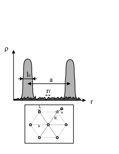
Figure 1: The three length characterizing the Wigner crystal. The size $l_{c}$ of the “particles” in the crystal (at low temperature it is essentially given by the extension of the wavefunction around the equilibrium position and is the cyclotron radius, at large temperatures it is controlled by the thermal fluctuations and is the Lindemann length), $a$ the lattice spacing is controlled by the density of particles, and the disorder is correlated over a length $r_{f}$. The inset shows the triangular structure of the Wigner crystal. Particles are labeled by an equilibrium position ${R}_{i}$ and a displacement ${u}$.

The long wavelength properties of the WC can now be described by an elastic hamiltonian describing the displacements $u$. We set $\hbar=1$ in the rest of the paper. The vibration modes of this crystal can be quantized in the usual manner leading to the imaginary time elastic action in the presence of disorder,

$$S = \frac{1}{2}\int_{\bf q}\frac{1}{\beta}\sum_{\omega_{n}}u_{\alpha}(q,\omega_{n})[(\rho_{m}\omega_{n}^{2}+cq^{2})\delta_{\alpha\beta}+d\frac{q_{\alpha}q_{\beta}}{q}$$

$$+i\rho_{m}\omega_{n}\omega_{c}\epsilon_{\alpha\beta}]u_{\beta}(-q,-\omega_{n})$$

$$+\int d^{2}r\int_{0}^{\beta}d\tau V({r})\rho({r},\tau)$$

where here and below we denote the integration over the Brillouin zone (BZ)

$$\int_{\bf q}=\int_{BZ}\frac{d^{2}q}{(2\pi)^{2}}$$ (2)

and $u_{\alpha}$ with $\alpha=x,y$ are the two components of the vector $u$, $\epsilon_{\alpha\beta}$ is the antisymmetric tensor $\epsilon_{xy}=-\epsilon_{yx}=1$ and the Matsubara frequencies $\omega_{n}=\frac{2\pi n}{\beta}$ with the inverse temperature $\beta=1/T$. $\rho_{m}\simeq{m\over{\pi a^{2}}},\rho_{c}\simeq{e\over{\pi a^{2}}}$ are the mass and charge densities. $c$ and $d$ are the shear and bulk moduli. These moduli can be obtained from an expansion of the coulomb correlation energy of the WC in terms of the displacements. Analytical expressions for the elastic moduli were obtained for the classical crystal in Ref. Bonsall and Maradudin, 1977. Later, efforts were made to estimate quantum corrections to these moduli using trial wave functionsMaki and Zotos (1983). Here, we work with the classical values obtained in Ref. Bonsall and Maradudin, 1977 where the elastic moduli are independent of the magnetic field, which should be a reasonable approximation for strong fields. The bulk modulus $d$ and the shear modulus $c$ are given by

$$d = \frac{\rho_{c}^{2}}{\epsilon}$$ (3)

$$c = \alpha\frac{\rho_{c}^{2}a}{\epsilon}$$ (4)

where $\alpha\simeq 0.03$ and $\epsilon$ is the dielectric constant of the substrate. Since the bulk modulus describes compressional modes, it is drastically affected by the coulomb repulsion. The off-diagonal term in the action (II.1) comes from the Lorentz force, and is proportional to the cyclotron frequency $\omega_{c}={{\rho_{c}B}/{\rho_{m}}}$, where $B$ is the magnetic field applied perpendicular to the plane of the crystal. Finally, the last term describes the coupling to disorder, modeled here by a random potential $V$. The density of particles

$$\rho({r})=\sum_{i}\overline{\delta}({r}-{R}_{i}-{u}_{i})$$ (5)

where $\overline{\delta}$ is a $\delta$-like function of range $l_{c}$ (see Figure 1) and ${u}_{i}\equiv{u}({R}_{i})$. Since the disorder can vary at a lengthscale $r_{f}$ a priori shorter or comparable to the lattice spacing $a$, the continuum limit ${u}_{i}\to{u}(r)$, valid in the elastic limit $|{u}_{i}-{u}_{i+1}|\ll a$ should be taken with care in the disorder term Giamarchi and Le Doussal (1994, 1995). This can be done using the decomposition of the density in terms of its Fourier components

$$\rho({r})\simeq\rho_{0}-\rho_{0}\nabla\cdot{u}+\rho_{0}\sum_{{K}\neq 0}e^{i{K}\cdot({r}-{u}(r))}$$ (6)

where $\rho_{0}$ is the average density and ${K}$ are the reciprocal lattice vectors of the perfect crystal. The finite range of $\overline{\delta}$ is recoveredGiamarchi and Le Doussal (1995) by restricting the sum over $K$ to momentum of order $K_{\rm max}\sim\pi/l_{c}$ We assume a gaussian distribution for the disorder $V(r)$, which leads to the following disorder averages

$$\overline{V({r})V({r}^{\prime})}=\Delta_{r_{f}}({r}-{r}^{\prime})$$ (7)

$\Delta_{r_{f}}$ is a delta-like function of range $r_{f}$ which is the characteristic correlation length of the disorder potential (see Figure 1). The gaussian limit is valid when there are many weak pins. We will come back to this point in a more quantitative manner in the next section.

II.2 Physical lengthscales

The physical properties of the various phases of the two dimensional electron crystal are completely governed by the interplay of the the various microscopic length scales in the system: the lattice spacing $a$, the particle size $l_{c}$ and the disorder correlation length $r_{f}$. These microscopic parameters define collective lengthscales which are of fundamental importance in the physics of such disordered systems Giamarchi and Le Doussal (1995, 1998); Giamarchi and Orignac (2000). These length scales, $R_{c}$ and $R_{a}$, are the distances over which the relative displacements are of the order of the size of the particle and the lattice spacing respectively. They are defined by the disorder averaged displacement correlation functions

$$\langle[{u}({R}_{c})-{u}({0})]^{2}\rangle = \text{max}[r_{f}^{2},l_{c}^{2}]\equiv\xi^{2}_{0}$$ (8)

$$\langle[{u}({R}_{a})-{u}({0})]^{2}\rangle = a^{2}$$

In order to distinguish between these two lengths it is mandatory to keep all the harmonics in the decomposition of the density (6). Keeping only one harmonic, as is done for CDW, amounts to considering that the effective “size” of the particle is $a$ and hence $R_{c}\sim R_{a}$. For the Wigner crystal, as we will see, it is crucial to carefully distinguish between these two lengthscales.

The length $R_{a}$ can easily be obtained by a static scaling argument comparing the cost in shear elastic energy and the gain due to disorder. For the WC, where $n\simeq(\pi a^{2})^{-1}$ we get

$$R_{a}={{ca^{2}}\over{n\sqrt{\Delta}}}$$ (9)

In order to be in the weak pinning regime, and for an elastic description to be valid, it is necessary to have $R_{a}\gg a$.

The interpretation of $R_{c}$, the so called Larkin-Ovchinikov lengthLarkin and Ovchinnikov (1979) is more subtle. It corresponds to lengths where the particles can truly feel the random potential. In particular, it is the length above which the Larkin model Larkin (1970), which approximates the random potential by a random force becomes invalid, and pinning and metastability appear. If $R_{c}\gg a$, the system is collectively pinned, whereas one would have single particle pinning in the opposite case. We emphasize that the elastic approximation is valid regardless of the behavior of $R_{c}$, provided one still has $R_{a}\gg a$.

Since $u(R_{a})\sim a$, $R_{a}$ has in the past been incorrectly interpreted as the lengthscale at which topological defects such as dislocations appear and the translational order of the crystal is lost. The naive picture is the one of a crystal broken into crystallites of size $R_{a}$. It has recently been shown that this view is grossly incorrect. In particular, even in two dimension topological defects appear at a lengthscale $R_{D}$ much greater than $R_{a}$, and the crystal preserves a very good degree of positional order Giamarchi and Le Doussal (1995); Le Doussal and Giamarchi (2000). In three dimensions, the situation is even more favorable since the system preserves a quasi translational order (power-law divergent Bragg peaks) and topological defects are not generated by weak disorder ($R_{D}=\infty$). The physical implications of these results for the present problem will be discussed in section VI.4.

III GVM

III.1 Method

We now study the disordered WC described by (II.1). Due to the nonlinear coupling of the disorder to the displacement field $u$ in (II.1), this problem is extremely difficult to solve. Here, we treat it using a variational method Giamarchi and Le Doussal (1996a); Chitra et al. (1998). Many of the technical details and subtleties of the method can be found in the literature (see e.g. Ref. Giamarchi and Le Doussal, 1998; Giamarchi and Orignac, 2000 for a review). We focus directly on the WC and we present here only the main steps. The first step involves averaging (II.1) over disorder by introducing replicas. This averaging results in an effective action which involves interactions between the $n$ replicas, given by

$$S = \frac{1}{2}\sum_{\omega_{n}}\int_{\bf q}\sum_{a}u_{\alpha}^{a}(q,\omega_{n})\left[(\rho_{m}\omega_{n}^{2}+cq^{2})\delta_{\alpha\gamma}+i\rho_{m}\omega_{n}\omega_{c}\epsilon_{\alpha\gamma}+d\frac{q_{\alpha}q_{\gamma}}{q}\right]u^{a}_{\gamma}(-q,-\omega_{n})$$ (10)

$$-\frac{\rho_{0}^{2}}{2}\int d^{2}r\int_{0}^{\beta}\int_{0}^{\beta}d\tau d\tau^{\prime}\sum_{a,b,{K}}\Delta_{K}\cos\left[K\cdot\left(u^{a}({r},\tau)-u^{b}({r},\tau^{\prime})\right)\right]$$

where summations over $\alpha$ and $\beta$ are implicit. The replica indices, $a,b$ run from $1$ to $n$. ${K}$ denotes the reciprocal lattice vectors. The size of the particles $l_{c}$ and the finite correlation length of the disorder restrict the sum over ${K}$ to values of $K$ smaller than $K_{\rm max}\sim\pi/\max(r_{f},l_{c})$. $\Delta_{K}$ is taken as a constant $\Delta_{K}=\Delta$ for $K<K_{\rm max}$ and zero otherwise. A more precise formulation is given in Appendix A. The physical disorder averages are recovered in the limit $n\to 0$. (10) is quite general and can be used to describe a host of physical systems, both quantum and classical Giamarchi and Orignac (2000).

The disorder couples the various replicas via the cosine term. Though this cosine term is local in space, it is completely non-local in time. This non-locality leads to a rich dynamical behavior as we shall show in this paper. In addition to the cosine term, another quadratic term is generated by the $q=0$ part of the disorder. This can be absorbed in a shift of the displacement field $u$. It affects the static correlation functions but not the transport properties and thus we neglect it henceforth.

We now search for a variational solution to (10) by using the best quadratic action approximating (10). We use the trial action

$$S_{0}=\frac{1}{2\beta}\int_{{\bf q}}\sum_{n}u_{\alpha}^{a}(q,\omega_{n})G^{{ab}-1}_{\alpha\beta}(q,\omega_{n})u_{\beta}^{b}(-q,-\omega_{n})$$ (11)

where the whole Green’s function $G^{{ab}-1}_{\alpha\beta}(q,\omega_{n})$ are variational parameters. The variational free energy is now given by

$$F_{\rm var}=F_{0}+\langle S-S_{0}\rangle_{S_{0}}$$ (12)

The variational parameters are then determined by the saddle point equations

$$\frac{\partial F_{\rm var}}{\partial G^{{ab}-1}_{\alpha\beta}(q,\omega_{n})}=0$$ (13)

The explicit form of these equations are given in Appendix B.

III.2 Saddle point equations

The saddle point equations (13) have to be solved in the limit of the number of replicas $n\to 0$. There are two kinds of saddle point solutions in general: one with replica symmetry and the other with replica symmetry breaking. For the case of interest here, $d=2$, one can show that the correct way to take the limit $n\to 0$ is to break the replica symmetry Giamarchi and Le Doussal (1996a). We first introduce the displacement correlation function

$$B_{\alpha\beta}^{ab}({x},\tau) = \langle[u_{\alpha}^{a}({x},\tau)-u_{\beta}^{b}({0},0)]^{2}\rangle=\frac{\beta}{\int}_{\bf q}\sum_{n}\left(G_{\alpha\beta}^{aa}(q,\omega_{n})+G_{\alpha\beta}^{bb}(q,\omega_{n})-2\cos(qx+\omega_{n}\tau)G_{\alpha\beta}^{ab}(q,\omega_{n})\right)$$ (14)

We then parametrize the replica Green’s function as follows:

$$[G^{-1}]^{\alpha\beta}_{ab}(q,\omega_{n})=f^{\alpha\beta}(q,\omega_{n})\delta_{ab}+\sigma^{\alpha\beta}_{ab}(\omega_{n})$$ (15)

where $\sigma$ are the variational parameters and $f^{\alpha\beta}(q,\omega_{n})$ is the elastic matrix defined in (II.1). Since the disorder induced interaction between replicas is local in space and non-local in time, the parameters $\sigma$ depend only on the frequency. We now define the connected part of the Green’s functions as

$$G_{c}^{\alpha\beta}(q,\omega_{n})=\sum_{b}G^{\alpha\beta}_{ab}(q,\omega_{n})$$ (16)

The saddle point equations, the $f_{\alpha\beta}$ and the various connected Green’s functions are all given in the appendix B.

The matrix structure of the saddle point equations simplify if we use the basis of longitudinal and transverse displacements. This offers a physically transparent picture in that the transverse modes are the shear modes of the solid and the longitudinal ones represent the compression modes. In this basis, the Cartesian displacements are given by

$$u_{\alpha}(q)=u^{L}(q)\hat{q}_{\alpha}+u^{T}(q)\epsilon_{\alpha\beta}\hat{q}_{\beta}$$ (17)

where $\hat{q}=q/|q|$ is the unit vector along $q$. For the pure system, in the absence of a magnetic field, the longitudinal and transverse modes are the eigenmodes of the system. The longitudinal mode is sensitive to the Coulomb repulsion whereas the transverse mode is not. The non-disordered part of the Hamiltonian can be rewritten as

$$S[u] = \int_{\bf q}\sum_{n}[u^{L}_{q,\omega_{n}}(\rho_{m}\omega_{n}^{2}+cq^{2}+dq)u^{L}_{-q,-\omega_{n}}$$ (18)

$$+u^{T}_{q,\omega_{n}}(\rho_{m}\omega_{n}^{2}+cq^{2})u^{T}_{-q,-\omega_{n}}$$

$$+\rho_{m}\omega_{c}\omega_{n}(u^{L}_{q,\omega_{n}}u^{T}_{-q,-\omega_{n}}-u^{L}_{-q,-\omega_{n}}u^{T}_{q,\omega_{n})}]$$

The magnetic field mixes these two modes. Note that the longitudinal mode yields the correct dispersion for the plasmon mode $\omega\sim q^{1/2}$. Though the disorder term in (10) has a complicated form in terms of $u_{L}$ and $u_{T}$, the saddle point equations themselves can be easily written in terms of these longitudinal and transverse modes. Since, the appropriate solution is the replica symmetry broken one, all quantities which are off-diagonal in the replica indices are parametrized in terms of a continuous variable $0\leq u\leq 1$. There is a break-point $u_{c}$ such that for $u<u_{c}$ the solutions manifest explicit replica symmetry breaking and one recovers effectively replica symmetric solutions for $u>u_{c}$. The saddle point equations, their parametrisation in terms of $u$, the structure of the various replica Green’s functions are all discussed elaborately in Appendix B.

In this section, we present only the final version of these equations. These equations contain a parameter $\Sigma$ which can be seen as a disorder induced mass gap and the function $I(i\omega_{n})$ which describes essentially the dissipation due to disorder. In terms of these new variables, the various connected Green’s functions are now given by

$$G_{cT}(q,i\omega_{n}) = {{cq^{2}+dq+{\rho_{m}}\omega_{n}^{2}+I(i\omega_{n})+\Sigma(1-\delta_{n,0})}\over{[(cq^{2}+dq+{\rho_{m}}\omega_{n}^{2}+I(i\omega_{n})+\Sigma(1-\delta_{n,0}))(cq^{2}+{\rho_{m}}\omega_{n}^{2}+I(i\omega_{n})+\Sigma(1-\delta_{n,0}))+{\rho_{m}^{2}}\omega_{n}^{2}\omega_{c}^{2}]}}$$

$$G_{cL}(q,i\omega_{n}) = {{cq^{2}+{\rho_{m}}\omega_{n}^{2}+I(i\omega_{n})+\Sigma(1-\delta_{n,0})}\over{[(cq^{2}+dq+{\rho_{m}}\omega_{n}^{2}+I(i\omega_{n})+\Sigma(1-\delta_{n,0}))(cq^{2}+{\rho_{m}}\omega_{n}^{2}+I(i\omega_{n})+\Sigma(1-\delta_{n,0}))+{\rho_{m}^{2}}\omega_{n}^{2}\omega_{c}^{2}]}}$$ (19)

$$G_{cLT}(q,i\omega_{n}) = {{{\rho_{m}}\omega_{n}\omega_{c}}\over{[(cq^{2}+dq+{\rho_{m}}\omega_{n}^{2}+I(i\omega_{n})+\Sigma(1-\delta_{n,0}))(cq^{2}+{\rho_{m}}\omega_{n}^{2}+I(i\omega_{n})+\Sigma(1-\delta_{n,0}))+{\rho_{m}^{2}}\omega_{n}^{2}\omega_{c}^{2}]}}$$

where $I(i\omega_{n})$ satisfies (in the semi-classical limit)

$$I(i\omega_{n}) = 2\pi c\Sigma\int_{\bf q}\left[{1\over{cq^{2}+\Sigma}}+{1\over{cq^{2}+dq+\Sigma}}\right.$$ (20)

$$\left.-{{2(cq^{2}+\omega_{n}^{2}+I(i\omega_{n})+\Sigma)+dq}\over{(cq^{2}+\rho_{m}\omega_{n}^{2}+dq+I(i\omega_{n})+\Sigma)(cq^{2}+\rho_{m}\omega_{n}^{2}+I(i\omega_{n})+\Sigma)+\rho_{m}^{2}\omega_{n}^{2}\omega_{c}^{2}}}\right]$$

and the equation determining $\Sigma$ is

$$\Sigma=\sum_{K}\rho_{0}^{2}\Delta_{K}\frac{{K}^{2}}{4\pi}e^{-\frac{1}{2}{K}^{2}B(u_{c})}$$ (21)

The term in the exponential, $B(u_{c})$, is given by

$$B(u_{c}) = {1\over\beta}\int_{\bf q}\left[\sum_{n\neq 0}\left(G_{cL}(q,\omega_{n})+G_{cT}(q,\omega_{n})\right)\right.$$ (22)

$$\left.+{1\over{cq^{2}+dq+\Sigma}}+{1\over{cq^{2}+\Sigma}}\right]$$

where the breakpoint is

$$\beta u_{c}={{K^{2}}\over{8\pi c}}$$ (23)

(determined in Appendix B). Since (21) depends on $I$ through $B(u_{c})$, (19), (20) and (21) form a closed set of self consistent equations.

IV Solution of saddle point equations

We now solve the self consistent equations derived in the previous section. Before, we proceed with the explicit determination of the solution, let us examine some of the general features of the solution. A cursory glance at the propagator (19), shows that the mass term $\Sigma$ defines a lengthscale through $\Sigma=cl^{-2}$. As explained in Ref. Giamarchi and Le Doussal, 1995, this is the length scale which separates the Larkin regime from the random manifold regime. These two regimes are characterised by a power law growth of displacements with differing exponents. Moreover, at zero temperature, in the absence of thermal fluctuations the relative displacement correlation function, $\tilde{B}_{T}(l)\propto{\rm max}[l_{c}^{2},r_{f}^{2}]$. Comparing with (8), we immediately see that $l=R_{c}$ or equivalently,

$$\Sigma=cR_{c}^{{-2}}$$ (24)

where, $R_{c}$ is the Larkin-Ovchinikov length. Contrary to older theories of CDW, $\Sigma$ is related to $R_{c}$ and not the positional length $R_{a}$. We emphasize that $\Sigma=cR_{c}^{-2}$ only in the collective pinning regime where $R_{c}\gg a$. The equivalence $l=R_{c}$ fails when the system enters the single particle pinning regime where $R_{c}<a$.

IV.0.1 Results for $\Sigma$ and $R_{c}$

To solve for $\Sigma$, it is useful to remark that the structure of the equation (21), is very similar to the analogous equation for a classical system with point-like disorder. This allows us to directly apply the formalism developed in Ref. Giamarchi and Le Doussal, 1995 to the present problem. Re-arranging the terms in (75), we can see that $B(u_{c})$ is the extent of localization of the particle. Therefore, to leading order, we replace $B$ in (21) by $l_{c}^{2}$ which gives

$$\Sigma=c(2\pi^{2})^{-{1\over 6}}R_{a}^{-2}(a/\xi_{0})^{6}$$ (25)

where

$$\xi_{0}=\text{max}[r_{f},l_{c}]$$ (26)

The Larkin length $R_{c}$ is given by

$$R_{c}=R_{a}(\frac{\xi_{0}}{a})^{3}$$ (27)

We see from (25), that $\Sigma$ exhibits very different magnetic field dependences in the two physically distinct cases of $r_{f}><l_{c}$. We see that for $r_{f}\gg l_{c}$, $\Sigma$ is independent of the magnetic field and for $r_{f}\ll l_{c}$, $\Sigma=bB^{3}$, where reinstating $\hbar$, $b=c(2\pi^{2})^{-{1\over 6}}R_{a}^{-2}(a^{2}e/\hbar)^{3}$ (at $T=0$). This has extremely interesting ramifications for experimentally measurable quantities as we discuss in the following sections.

Let us illustrate the importance of retaining all the harmonics in the case where disorder varies at length scales smaller than $a$. If we retain only the lowest harmonic in (21), we would have $r_{f}=a$ since disorder now varies only on scales comparable to $a$. In the relevant limit, $l_{c}<a$, we see that the exponential in (21) can be replaced by unity. In other words, this corresponds to substituting $\xi=r_{f}\equiv a$ in (25) leading to the result that $R_{c}=R_{a}$. This precludes the possibility of any dependence of $\Sigma$ on the magnetic field because $R_{a}$ is a static scale independent of $B$. Thus we see that when disorder varies at scales smaller than $a$ i.e., $r_{f}<a$, it is necessary to retain all the harmonics in (21) to obtain the correct result for $\Sigma$.

IV.0.2 Behavior of $I(\omega)$

Though we have solved the equation determining $\Sigma$ in the full quantum sense, (73) proves difficult to solve. We thus examine the semi-classical limit given by (20). As was shown in simpler cases Giamarchi and Le Doussal (1996a), this limit captures correctly the main features of the solution. (20) is analytically solvable for small and large frequencies and can be solved numerically for intermediate frequencies. Two frequency scales control the behavior of $I(\omega_{n})$: (i) the pinning frequency $\omega_{p}^{0}={\Sigma}/\rho_{m}\omega_{c}$, to be discussed in detail in section VI; (ii) the cyclotron frequency $\omega_{c}$. For small $\omega_{n}$ ($\omega_{n}\ll{\frac{\Sigma}{\rho_{m}\omega_{c}}})$ , one gets

$$I(i\omega_{n})=\sqrt{2\rho_{m}\Sigma+{{\pi\rho_{m}^{2}\omega^{2}_{c}(c\Sigma)^{1\over 2}}\over{2d}}}|\omega_{n}|$$ (28)

As expected $I(i\omega_{n})\to 0$ when $\omega_{n}\to 0$. In the limit of small $\omega_{c}$, the second term inside the square root can be nelegected and we obtain the usual result for a system in a zero magnetic field. On the other hand, the second term dominates the low frequency behavior of $I$, if

$$\omega_{c}^{2}\gg\frac{4d}{\pi\rho_{m}}\sqrt{\frac{\Sigma}{c}}=\Omega\sqrt{\frac{\Sigma}{\rho_{m}}}$$ (29)

This defines a frequency scale, $\Omega^{2}\sim\frac{d^{2}}{\rho_{m}c}$. We work in the limit of large magnetic fields, $\rho_{m}\omega_{c}^{2}\gg\Sigma$. Since the two elastic moduli are related $d\propto\frac{c}{a}$, $\Omega^{2}\propto\frac{c}{m^{*}}$, where $m^{*}$ is the effective mass of the system. This clearly shows that $\Omega$ is just the plasma frequency of the two dimensional WC.

For intermediate frequencies $\sqrt{\frac{\Sigma}{\rho_{m}}}\ll\omega\ll\frac{\Omega^{2}}{\omega_{c}}$, the solution becomes

$$I(\omega_{n})\simeq{\Sigma\over 6}\log{{{\rho_{m}^{2}\omega_{n}^{2}}\omega_{c}^{2}}\over{d\Sigma^{3\over 2}}}$$ (30)

The analytical solutions given above, were obtained in the limit of $\rho_{m}\omega_{c}^{2}\gg\Sigma$. To obtain the solution numerically, we first continue (20) to real frequencies $\omega$, which results in a set of two coupled integral equations for the real and imaginary parts $I_{1}$ and $I_{2}$ of $I(\omega)$. These integral equations can be easily solved numerically. The numerical solutions indicate that the linear solution (28) obtained for frequencies $\omega\ll\Sigma/\rho_{m}\omega_{c}$, infact survives beyond this regime.

Figure 2: A generic numerical solution for the real $I_{1}(\omega)$ and imaginary $I_{2}(\omega)$ parts of $I(\omega)$ (in units of $\Sigma$) as a function of $\omega$ (in units of $\sqrt{\Sigma/\rho_{m}}$). Results for two different values of $\omega_{c}$ are shown. The corresponding value of $\omega_{p}^{0}\equiv\Sigma/\rho_{m}\omega_{c}$ is also given.

The numerical approach, however, is not constrained to this regime and can be used to obtain $I$ for all ranges of $\Sigma$ and $\omega_{c}$. Typical plots of $I_{1}$ and $I_{2}$ are shown on Figure 2. We see from Fig.2, that $I_{2}$ is indeed linear in $\omega$ and $I_{1}$ is quadratic for small $\omega$, in agreement of the analytical continuation of (28).

V Physical Properties - Statics

V.1 Compressibility

One of the few thermodynamic properties that can be measured in the QHE and MOSFET systems is the static compressibility $\kappa$ of the Wigner crystal. The formalism used in this paper allows us to calculate the static compressibility of the disordered crystal. The calculation of $\kappa$ requires a knowledge of the density-density correlation function.

$$\kappa=\lim_{q\to 0}\lim_{\omega\to 0}\Pi(q,\omega)$$ (31)

where the density operator is given by $\partial_{\alpha}u_{\alpha}=q_{\alpha}u_{\alpha}$. Clearly, only the longitudinal components of the displacement field contribute to the density. Consequently, the density correlation is entirely determined by the correlation of the longitudinal displacements and is given by

$$\Pi(q,\omega)=\rho_{0}^{2}q^{2}\langle u_{L}(q,\omega)u_{L}(-q,-\omega)\rangle$$ (32)

First let us consider the pure case. We immediately see that since the coulomb term $dq$ dominates over the shear term for small $q$, the compressibility $\kappa=0$ in the pure system. Consequently, the compressibility remains zero even in the disordered phase. We reiterate that the compressibility calculated here is related to the second derivative of the energy with respect to density for fixed total number of particles. This also assumes that the neutralising background remains unchanged as the volume of the electron gas is changed. Before comparing these results with experiments, it should be ascertained whether the compressibility measured in the experiment is the same quantity defined above Eisenstein et al. (1994).

V.2 Translational order

It is interesting to study the effect of disorder on the translational long range order present in the clean system at zero temperature. Contrary to the naive view based on extrapolation of Larkin Larkin (1970) and FL Fukuyama and Lee (1978a) methods that the crystal loses its long range order due to pinning, it was shown that in $d=3$ the disordered system, although pinned, retains a defect-free quasi-long range translational order. In $d=3$, this Bragg glass phase has thus power-law divergent Bragg peaks Giamarchi and Le Doussal (1995, 1998). For $d=2$ classical systems it is known that topological defects do appear but at a length $R_{d}$ which is much larger than $R_{a}$ and thus the elastic description holds in a large regime of length scales (up to $R_{D}$) resulting in a quasi Bragg glass state. The properties of the $d=2$ quasi Bragg glass for the classical problem have been studied in detail and the length scale $R_{D}$ has been estimated Giamarchi and Le Doussal (1995); Carpentier and Le Doussal (1997, 1998); Le Doussal and Giamarchi (2000).

We now derive the result given by the variational method for the positional correlation functions of the pinned WC in $d=2$.

$${\tilde{B}}_{L,T}(x,t=0) = {{2}\over{\beta u_{c}}}\int\int{{qdqd\theta}\over{(2\pi)^{2}}}d\omega\left[\cos^{2}\theta(1-\cos(qx\cos\theta)){{\Sigma\delta_{\omega=0}}\over{G_{cL,T}(G_{cL,T}+\Sigma)}}\right.$$ (33)

$$+\left.(1-\cos^{2}\theta)(1-\cos(qx\cos\theta)){{\Sigma\delta_{\omega=0}}\over{G_{cT,L}(G_{cT,L}+\Sigma)}}\right]$$

Since the equal time asymptotic behavior is governed primarily by $\omega=0$, it is sufficient to retain this mode alone in (33). We find that the leading contribution to the correlation function grows logarithmically i.e.,

$${\tilde{B}}_{L,T}(x)\simeq{\over{2\pi c\beta u_{c}}}\log\left({x\sqrt{\Sigma\over c}}\right)$$ (34)

Substituting (23) in the above and using the relation $\Sigma=cR_{c}^{-2}$ at zero temperature, (34) simplifies to

$${\tilde{B}}_{L,T}(x)\simeq{4\over{{K}_{0}^{2}}}\log\left({x\over{R_{c}}}\right)$$ (35)

Only the leading contribution to the displacements grow in an isotropic manner. There are non-isotropic corrections to this result but these can be neglected in the asymptotic limit. The translational correlation is given by

$$O_{T}=\langle\exp^{i{K}_{0}.{u}(x)}\exp^{-i{K}_{0}.{u}(0)}\rangle$$

Within the Gaussian approximation used in this paper

$$O_{T} = \exp[-{{K_{0\alpha}K_{0\beta}}\over 2}{\tilde{B}}_{\alpha\beta}(x)]$$ (36)

$$\simeq \left({{R_{c}}\over x}\right)^{2}$$

thus the pinned WC also supports quasi long range order. Since $R_{c}$ is determined by (27), we see from (34) that the growth of displacements will have a magnetic field dependence depending on whether $r_{f}$ is lesser or greater than $l_{c}$. The $B$ dependence in a static correlation function like the one studied here is a direct consequence of the fact that in the quantum system the statics and the dynamics are coupled.

Although the GVM correctly captures several features of the growth of displacements in $d=2$, it should be taken with a grain of salt concerning the exact asymptotic behavior. It is well known for the classical problem that the variational method slightly underestimates the fluctuations at the lower critical dimension $d=2$ and that the variational result $\log(r)$ should in fact be replaced by $\log^{2}(r)$. The latter result can be derived by a more accurate renormalization group approach Cardy and Ostlund (1982); Giamarchi and Le Doussal (1995); Carpentier and Le Doussal (1997); Giamarchi and Le Doussal (1998). It is fair to expect that the result will be similar for the quantum problem considered here, since the $\omega=0$ mode considered in (33) mimics a $d=2$ classical problem. Despite this, even a $\log^{2}$ growth of the correlation functions would lead to an extremely weak destruction of the positional order, in the quantum case analogous to the quasi Bragg glass. The other important question is the role of dislocations. Again the precise answer is only known for the classical problem, for which it has been shown that in $d=2$ dislocation are generated but at a lengthscale $R_{D}$ much larger Giamarchi and Le Doussal (1995) than $R_{a}$. In particular the result at zero temperature, relevant for the ground state, reads Le Doussal and Giamarchi (2000); Carpentier and Le Doussal (2000):

$$R_{D}\sim R_{a}e^{c\sqrt{(\frac{1}{8}-\sigma_{0})\ln(R_{a}/a)}}$$ (37)

where $\sigma_{0}$ is proportional to the strength of disorder. For the pinned WC the effect of additional quantum fluctuations and Coulomb interactions remains to be treated in a precise way. As can be seen e.g. by analogy to a 3d classical system with correlated disorder (where it is known that fluctuations play a minor role), one can surmise that (37) should be rather stable to small quantum fluctuations. Consequently, the pinned WC should still exhibit an extremely good positional order for weak disorder.

VI Physical Properties - Dynamics

VI.1 General features of the conductivity

The formalism and the results obtained in the previous sections can now be used to calculate the magneto-conductivities of the pinned crystal. The conductivities are given by

$$\sigma_{\alpha\beta}(\omega)=i\rho_{c}^{{2}}\omega G_{\alpha\beta}(q=0,\omega+i\epsilon)$$ (38)

$\alpha,\beta=x,y$ and the $G$ are the displacement Green’s function. The real frequencies $\omega$ are analytic continuations of the Matsubara frequencies $\omega_{n}$. Using (B), the explicit form of the conductivities are

$$\sigma_{xx} =\sigma_{yy} =\rho_{c}^{{2}}{{i\omega[-\rho_{m}\omega^{2}+\Sigma+I(\omega)]}\over{(\Sigma-\rho_{m}\omega^{2}+I(\omega))^{2}-\rho_{m}^{2}\omega_{c}^{2}\omega^{2}}}$$

$$\sigma_{xy} =-\sigma_{yx} =\rho_{c}^{2}{{\omega[\rho_{m}\omega\omega_{c}]}\over{(\Sigma-\rho_{m}\omega^{2}+I(\omega))^{2}-\rho_{m}^{2}\omega_{c}^{2}\omega^{2}}}$$ (39)

The conductivity tensor is therefore, completely determined by $\Sigma$ and $I(\omega)$. As usual the Hall resistivity is given by

$$R_{H}={{\sigma_{xy}}\over{\sigma_{xx}^{2}+\sigma_{xy}^{2}}}$$ (40)

For the pure system, $\Sigma=I=0$ and (39) gives back the standard features of electrons in a magnetic field. The Drude peak is shifted by the magnetic field from $\omega=0$ to the cyclotron frequency $\omega_{c}$. The d.c. Hall conductivity has a finite value $\sigma_{xy}(\omega=0)=\rho_{c}/B$, and the Hall resistivity has the classical value $R_{H}=B/\rho_{c}$.

In the presence of disorder ($\Sigma\neq 0$, $I(\omega)\neq 0$), as can be seen from (39), the $\delta$-function peak at $\omega_{c}$ will broaden and slightly shift in frequency. (39) also shows that the dc conductivities $\sigma_{xx}(\omega=0)=\sigma_{yy}(\omega=0)=\sigma_{xy}(\omega=0)=0$, both in the presence and absence of a magnetic field. This is a consequence of the crystal being pinned by disorder. More importantly, a new peak appears in the diagonal conductivity at new scale $\omega_{p}$ called the pinning frequency.

A simple estimate of the pinning frequency is given by the poles in the conductivity when setting $I(\omega)=0$. This gives a $\omega_{p}^{0}=(\sqrt{\omega_{c}^{2}+4\Sigma/\rho_{m}}-\omega_{c})/2$. In the limit of large magnetic fields, which is relevant for the case of quantum Hall systems, the above expression simplifies to

$$\omega_{p}^{0}={\Sigma\over{\rho_{m}\omega_{c}}}$$ (41)

The cyclotron peak is shifted to $\omega_{c}+\omega_{p}^{0}$. Of course $\omega_{p}^{0}$ is only an approximation to the true pinning frequency $\omega_{p}$ that should be determined directly by the maximum of the conductivity (39). The main difference between $\omega_{p}^{0}$ and $\omega_{p}$ stems from the presence of $I(\omega)$ in the denominator.

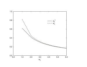
Figure 3: $r_{f}>l_{c}$: The pinning frequencies $\omega_{p}$ and $\omega_{p}^{0}$ as a function of $\omega_{c}$. All frequencies are in units of $\sqrt{\Sigma/\rho_{m}}$. Note that $\omega_{p}^{0}$ and $\omega_{p}$ become quite different for low magnetic fields.

Figure 4: $r_{f}<l_{c}$: The pinning frequencies $\omega_{p}$ and $\omega_{p}^{0}$ (in units of $\rho_{c}^{3}/\rho_{m}^{2}b$) as a function of the applied field $B$ (in units of $\rho_{c}^{2}/\rho_{m}b$). $b$ is defined in Sec. IV.0.1.

Typical values of the pinning frequencies are shown in Fig. 3 and Fig. 4.

Quite remarkably, the structure (39) of the conductivity tensor shows that the Hall resistivity $R_{H}$ is a constant independent of $\omega$

$$R_{H}=\frac{B}{\rho_{c}}$$ (42)

as in the pure system. This is a remarkable result since since it shows that the disorder has no influence on the Hall resistivity of a pinned WC. This property comes from the fact that the disorder is local, which in the variational calculation makes all off diagonal self energies zero, as explained in Appendix B. Since this feature is linked to the locality of disorder it is expected to be valid beyond the variational approximation.

We now analyze the frequency dependence of the conductivities. For small values of $\omega$, substituting (28) in (39) gives

$$Re\sigma_{xx}(\omega) = \rho_{c}^{2}{\sqrt{2\rho_{m}\Sigma+{{\pi\rho_{m}^{2}\omega^{2}_{c}(c\Sigma)^{1\over 2}}\over{2d}}}{{\omega^{2}}\over{\Sigma^{2}}}}$$

$$Re\sigma_{xy}(\omega) = \rho_{c}^{2}\rho_{m}\omega_{c}{({\omega\over\Sigma})^{2}}$$ (43)

and the imaginary or dissipative part of the conductivity grows as

$$Im\sigma_{xx}(\omega) = \rho_{c}^{2}{\omega\over\Sigma}$$

$$\ Im\sigma_{xy}(\omega) = \rho_{c}^{2}\rho_{m}^{3\over 2}{{\omega_{c}\omega^{3}}\over{\Sigma^{5\over 2}}}$$ (44)

In the region $\sqrt{\frac{\Sigma}{\rho}_{m}}\ll\omega\ll\frac{\Omega^{2}}{\omega_{c}}$ we find using (30)

$$Re\sigma_{xx}(\omega)\sim{\rho_{c}^{2}\over\rho_{m}^{2}}{\Sigma\over{\omega_{c}^{2}\omega}}\qquad Re\sigma_{xy}(\omega)\sim{\rho_{c}\over B}$$ (45)

The full behavior of the conductivity can be obtained from (39) by numerically solving the equation for $I(\omega)$. Typical plots of diagonal and transverse conductivities are shown in Fig. 5 and Fig. 6.

Figure 5: $r_{f}>l_{c}$: Re$\sigma_{xx}$ (in units of $\rho_{c}^{2}/\sqrt{\rho_{m}\Sigma}$) as a function of $\omega$ and $\omega_{c}$(in units of $\sqrt{\Sigma/\rho_{m}}$). Note the non Lorentzian shape of the peaks. In this regime, the pinning frequency decreases with increasing magnetic field.

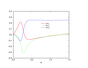
Figure 6: $r_{f}>l_{c}$: Im$\sigma_{xx}$,Re$\sigma_{xy}$ and Im$\sigma_{xy}$(in units of $\rho_{c}^{2}/\sqrt{\rho_{m}\Sigma}$) as a function of $\omega$ and $\omega_{c}$ (in units of ${\sqrt{\Sigma/\rho_{m}}}$) for $\omega_{c}^{2}=10$.

In the limit of very strong magnetic fields, since $\omega_{p}^{0}\ll\sqrt{\frac{\Sigma}{\rho_{m}}}\ll\omega_{c}$, provided $\omega_{c}^{2}\gg\Omega\sqrt{\frac{\Sigma}{\rho_{m}}}$ (see discussion in Sec. IV.0.2) the evolution of the width $\Delta\omega_{p}$ of the pinning peak is completely governed by the low frequency behavior of $I$ obtained in (28). In this limit,

$$\frac{\Delta\omega_{p}}{\omega_{p}}\propto\left(\frac{\Sigma}{n}\right)^{1/4}$$ (46)

Again from (25), we see that the behavior of the peak widths is again dictated by $r_{f}$ and $l_{c}$. A similar result was obtained in Ref. Fogler and Huse, 2000 with an undetermined exponent $s$ (to be discussed in Sec. VIII).

The case of zero external magnetic field can also be obtained from (39) by setting $\omega_{c}=0$. It leads to different energy scales and physical behavior. The clean crystal has infinite dc conductivity and zero ac conductivity. In the presence of disorder, the dc conductivity is zero as expected and a pinning peak develops at the frequency $\omega_{p}^{0}={\sqrt{\Sigma/\rho_{m}}}$ where $\Sigma$ is determined by (25) with $\xi=r_{f}$. We show a typical plot of the conductivity in Fig. 7.

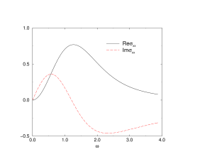
Figure 7: Re$\sigma_{xx}$ and Im$\sigma_{xx}$ (in units of $\rho_{c}^{2}/\sqrt{\rho_{m}\Sigma}$) as a function of $\omega$(in units of ${\sqrt{\Sigma/\rho_{m}}}$) for the pinned crystal in zero magnetic field.

An important feature of our results is that the pinning peaks are rather sharp for finite magnetic fields, as opposed to the rather broad pinning peak obtained in the limit of zero magnetic field. This is expected because the cyclotron peak in the former case has appreciable spectral weight. Comparing Fig. 7 and Fig. 5, we see that the peaks in the finite field case are at least a factor of 10-15 times narrower.

Moreover, the older theories predict a Lorentzian broadening of the peaks. A glance at the conductivities plotted in Figs.5,8 and 7 shows that the pinning peaks are non-Lorentzian and asymmetric around $\omega_{p}$. This is an important prediction of our theory. This asymmetry in the peak is indeed seen in microwave conductivity measurements on certain Ga-As samples Li and et al (1997, 2000); Beya (1998). Comparison of our results with experiments will be discussed in further detail in Sec. VII.

A generic property of pinned systems is that a finite nonzero threshold electric field $E_{T}$ is required before the crystal de-pins and d.c. current flows through the system. Since $E_{T}$ is intrinsically the signal of non-linear response, it cannot be directly evaluated using Kubo-like formulae. As for the dynamics of classical crystals Chauve et al. (1998, 2000), its precise calculation would require a non equilibrium formulation such as the Keldysh technique. This is clearly a formidable task, but fortunately for the classical cases, approximate derivations allow one to relate $E_{T}$ to equilibrium quantities. A dynamical derivation has shown that such formulas indeed yield the correct threshold field $E_{T}$. Here, we use the same approximate approach to derive $E_{T}$ for the quantum system. In the collective pinning regime, $R_{c}\gg a$, the threshold field $E_{T}$ is determined by $R_{c}$ Larkin and Ovchinnikov (1979)

$$E_{T}={c}R_{c}^{-2}\xi_{0}$$ (47)

where $\xi_{0}=\rm{max}[r_{f},l_{c}]$. Clearly, $E_{T}$ defined by (47) is directly linked to $\omega_{p}^{0}$ by $E_{T}=\rho_{m}\omega_{c}\omega_{p}^{0}\xi_{0}$. The validity of this result remains to be explicitly proven in the quantum case.

VI.2 Magnetic Field dependence

As already pointed out, it is crucial to have theoretical predictions for the various features and attributes of the conductivity as a function of physical parameters like the magnetic field and the density. This would then facilitate direct comparisons between experiment and theory and consequently further our understanding of the system.

It is clear from the previous section that $\Sigma$ and hence the length scale $R_{c}$ determine most of the dynamical properties of the pinned crystal. Different behaviors are possible depending on the relative magnitude of the correlation length of the disorder $r_{f}$ and the particle size $l_{c}$ (see Fig. 1). This leads to a physics very different from that predicted by the naive weak pinning scenario Fukuyama and Lee (1978a); Normand et al. (1992) where, it is implicitly assumed that the scale $R_{a}$ is the only lengthscale in the system. Two main behaviors can be obtained.

VI.2.1 $r_{f}>l_{c}$

In this case, the particle locally sees a smooth potential, and thus behaves effectively like a point particle. Hence the length $l_{c}$ is not directly relevant. This leads to a $R_{c}$ which is independent of the magnetic field, as was shown in Sec. IV. ¿From (25), one obtains for the naive pinning frequency

$$\omega_{p}^{0}(B)={{\Sigma}\over{\rho_{m}\omega_{c}}}=(2\pi^{2})^{-{1\over 6}}{{cR_{a}^{-2}}\over{\rho_{c}B}}({a\over{r_{f}}})^{6}$$ (48)

Consequently, the naive pinning peak moves towards the origin as $B^{-1}$ and gets narrower with increasing field. However, as mentioned in Sec. VI.1, the true pinning frequency is given by the location of the peak in the optical conductivity, and can be in principle different from $\omega_{p}^{0}$. A plot of the conductivity in this regime for different values of the magnetic field is shown in Fig. 5. From it we extract the true pinning frequency $\omega_{p}$. As seen in Fig. 3, both frequencies decrease as $B^{-1}$. We see that the difference $\omega_{p}-\omega_{p}^{0}$ is more pronounced for small values of $B$ or equivalently, $\omega_{c}^{2}/\Sigma$, and goes to zero for increasing values of the field $B$. Similarly, the non-Lorentzian nature of the peaks discussed earlier is enhanced for small and intermediate magnetic fields (cf. Fig. 5). The regime $r_{f}>l_{c}$ includes the case of the conventional CDW in a magnetic field for which $r_{f}\sim a$ and thus $R_{a}\simeq R_{c}$. Therefore, CDW have the same magnetic field dependence for the pinning frequency as the Wigner crystal in this regime. The density dependences are, however, quite different, as will be shown in Secs. VI.3 and VII.

VI.2.2 $r_{f}<l_{c}$

In this regime, since the size of the particle is larger than the correlation length of the disorder (see Fig. 1), the particle locally averages over the disorder. The effective disorder seen by the particle thus strongly depends on its size $l_{c}$. Since the particle size $l_{c}$ is strongly magnetic field dependent, this regime exhibits anomalous magnetic field dependence in all physical quantities. This physics is captured by the equations for $\Sigma$ (21). (25) indicates that $\Sigma$ is strongly $B$ dependent. This explicit magnetic field dependence results in a naive pinning frequency (we have reinstated $\hbar$)

$$\omega_{p}^{0}(B)=(2\pi^{2})^{-{1\over 6}}{{cR_{a}^{-2}B^{2}}\over{\rho_{c}}}({{ea^{2}}\over\hbar})^{3}$$ (49)

which increases quadratically with increasing field $B$. Therefore, unlike the previous case (48) where the pinning frequency and peak width were decreasing functions of $B$, here the pinning peak moves up and broadens with increasing field.

As was done in Sec. VI.2.1, it is important to extract the true pinning frequency and peak width from the full conductivity. $Re\sigma_{xx}$ has been plotted for various values of $B$ ranging intermediate fields to strong fields, in Fig. 8. In this regime, all curves are plotted for varying $\omega_{c}^{2}/\Sigma$. However, since $\Sigma\propto B^{3}$, $\omega_{c}^{2}/\Sigma\propto B^{-1}$, which implies that an increase in $\omega_{c}^{2}/\Sigma$ corresponds to a decrease in the magnetic field $B$. A plot of the true pinning frequency is shown in Fig. 4. One sees that in this case the shift in pinning frequency, compared to the naive expression (49) is quite important. As before, this difference is more pronounced for small and intermediate values of $\omega_{c}^{2}/\Sigma$ which contrary to the previous case, now corresponds to large values of the field $B$. In a similar vein, as seen in Fig.(8), the peaks become more and more non-Lorentzian for increasing $B$ i.e., decreasing $\omega_{c}^{2}/\Sigma$. Our result for the field dependence of $\omega_{p}$, shown in Fig. 4, can be compared with the experimental results. This point will be discussed in further details in Sec. VII.

Figure 8: $r_{f}<l_{c}$: Re$\sigma_{xx}$(in units of $b\rho_{m}/\rho_{c}$) as a function of $\omega$ (in units of $\rho_{c}^{3}/\rho_{m}^{2}b$; $b$ has been defined in the text). Note that increasing $\omega_{c}^{2}/\Sigma$ corresponds to decreasing magnetic fields.

As long as $r_{f}<l_{c}$, $\omega_{p}^{0}$ increases with $B$. This increase in the pinning frequency is not indefinite. Two effects can limit this regime. For sufficiently large $B$, since $l_{c}$ decreases with $B$ one will cross over to the regime of Sec. VI.2.1 for which $l_{c}<r_{f}$. Since from (25) and (24), $R_{c}$ decreases with increasing $B$, this regime is also limited by $R_{c}\simeq a$, below which the system is no longer in the collective pinning regime. In that case, the correspondence (24) between $R_{c}$ and $\Sigma$ no longer holds and the result (25) for $\Sigma$ is invalid. One should thus re-evaluate $\Sigma$ in this single particle pinning regime. Solving (21) in this regime, we find $\Sigma\propto B^{3\over 2}$ and

$$\omega_{p}^{{0}}\propto B^{1\over 2}$$ (50)

Which of the two crossovers ($l_{c}\sim r_{f}$ or $R_{c}\sim a$) occurs first depends on the strength of the disorder in the system considered.

VI.2.3 Summary of magnetic field dependence

In general, one can thus expect three regimes with dramatically different behaviors of experimentally measurable quantities. A summary of these regimes and their features is shown in Table 1. Contrary to the standard CDW case, for a Wigner crystal the pinning frequency can increase with the magnetic field provided one is in the regime $r_{f}<l_{c}$. In all the regimes, the height of the pinning peak decreases approximately as $B^{-1}$ with increasing field. As expected, the cyclotron peak at $\omega_{c}+\omega_{p}$ is not qualitatively affected by the relative magnitudes of $r_{f}$ and $l_{c}$ and always moves upwards with increasing $B$.

The difference between $\omega_{p}^{0}$ and $\omega_{p}$ that appears in the WC regime, urges a re-examination of the relation between the pinning frequency and the threshold field. Indeed if the formula (47) holds, the threshold field should be related to $\omega_{p}^{0}$ and not $\omega_{p}$. This would imply that in the WC regime, the pinning frequency and threshold field would not be linearly related. It would thus be interesting to have extended plots of $E_{T}$ vs the pinning frequency $\omega_{p}$, such as the ones of Ref. Williams and et al, 1991. Let us reiterate that although the pinning frequency $\omega_{p}$ can be systematically calculated, the expression (47) for the threshold field remains unverified in the quantum case. Assuming (47), the magnetic field dependence of the the threshold field $E_{T}$ and the dielectric constant defined by

$$\epsilon_{xx}=Im\sigma_{xx}/\omega$$ (51)

are summarized in Table. 1.

Regime	$\Sigma$	$\omega_{p}^{0}$	$E_{T}$	$\epsilon_{xx}$
$r_{f}>l_{c}$	$B^{0}$	$B^{-1}$	$B^{0}$	$B^{0}$
$r_{f}<l_{c}$	$B^{3}$	$B^{2}$	$B^{5\over 2}$	$B^{-3}$
$R_{c}<a$	$B^{3\over 2}$	$B^{1\over 2}$	$B$	$B^{-{3\over 2}}$
$n$ ($r_{f}><l_{c}$)	$n^{-\frac{1}{2}}$	$n^{-\frac{3}{2}}$	$n^{-\frac{1}{2}}$	$n^{\frac{5}{2}}$

Table 1: Magnetic field and density dependences of various dynamical quantities.

VI.3 Density dependence

Another way to probe the Wigner crystalline state is to fix the magnetic field and see how the pinning peak evolves as the density of electrons is varied slowly. The first thing to realize is that since $r_{f}$ and $l_{c}$ are both independent of the density, the density dependence of $\Sigma$ in (25) and hence $\omega_{p}^{0}$ are the same irrespective of the relative magnitudes of $r_{f}$ and $l_{c}$. The pinning frequency using (25) is given by

$$\omega_{p}^{0}={\pi\over{m\omega_{c}}}{{\epsilon_{0}\Delta}\over{e^{2}\xi_{0}^{6}}}{a}^{3}\propto n^{-{3\over 2}}$$ (52)

(52) shows that the pinning frequency increases as density is decreased. The width of the peak increases and the height of the pinning peak decreases as $n^{2}$ with decreasing $n$. This is analogous to the behavior seen for increasing $B$ when $r_{f}<l_{c}$. Accordingly, other dynamical quantities like $E_{T}$, $\epsilon_{xx}$ etc have the density dependences indicated in Table. 1.

VI.4 Limitations and dc conductivity

Before embarking on a comparison of our results with experiments, let us discuss the range of validity of our theory.

As already mentioned in Sec. II.1, the quantum nature of the original particle can be safely hidden in the parameters of the crystal hamiltonian, as long as the spatial extent of the particles remain small compared to the lattice spacing. One expects this to be valid even quite close to the melting transition of the WC. Of course, our approach does not allow for a very precise description of the melting properties, beyond the simple position of the transition, since this simplified description is incapable of taking into account the fermionic statistics and the incompressible quantum fluid that is the melted “crystal”.

An a priori limitation of our study, even in the insulating phase far from melting, is to know whether the elastic model is a satisfactory starting point to obtain the transport properties or whether defects (vacancies, interstitials, dislocations etc) should be taken into account from the start. Indeed if dislocations appear at a typical lengthscale $R_{D}$ they will strongly modify the results given by the elastic description for frequencies smaller than a characteristic frequency $\omega_{D}\propto R_{D}^{-1}$.

Older theories of disordered elastic systems suggest that due to the presence of disorder, defects are favored at the length $R_{a}$ for which displacements would become of order of the lattice spacing (see section II.2). If, as in FL description, the pinning peak would be associated with the length $R_{a}$, we see that dislocations would change most of the interesting optical conductivity and in particular the pinning peak. Such a situation is summarized in Figure 9(a).

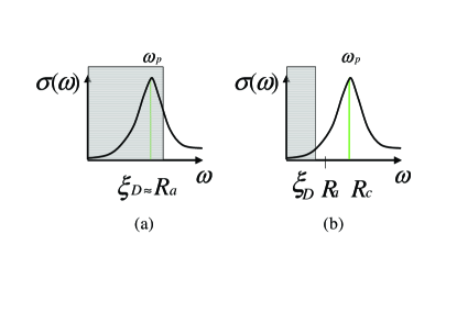
Figure 9: (a) If dislocations occurred at scale $R_{a}$ and the pinning frequency was controlled by $R_{a}$, as was naively believed, the elastic theory is incapable of giving any reliable information on the pinning peak. It would be necessary to include dislocations from the start. (b) As was shown in the text, dislocations occur in fact at $R_{D}\gg R_{a}$ and the pinning peak depends on $R_{c}\ll R_{a}$. Thus the pinning peak is given quantitatively by a purely elastic theory. It is necessary to take into account topological defects such as dislocations only at much lower frequencies, and in particular if one wants to obtain reliable results for the d.c. transport.

If this was correct this would seriously impair any description of the transport properties based on an elastic hamiltonian.

In fact, both of these commonly accepted points are incorrect, which makes the description based on an elastic model much more useful than initially anticipated. Firstly, as we already discussed in Sec. VI.1, the pinning peak is not associated with the length $R_{a}$ but with the a priori much smaller lengthscale $R_{c}$ (note that larger lengthscales correspond to smaller frequencies). Secondly, as discussed in Section V.2 defects in disordered elastic systems are much less important than initially believed and appear at a lengthscale $R_{D}$ much larger than $R_{a}$ ($R_{D}=\infty$ in $d=3$ for weak disorder). Since $R_{D}>R_{a}>R_{c}$, the frequency $\omega_{D}$ is thus much smaller than the characteristic frequencies of the pinning peak $\omega_{p}$. This implies that dislocations will not drastically affect the pinning peak and thus that the whole pinning peak structure is given quantitatively by the elastic model. This is summarized on Figure 9(b). Our study is thus perfectly adapted to describe optical conductivity experiments.

For d.c. transport or static properties the role played by topological defects is less obvious. In particular, it is reasonable to assume that they can have an impact on some of the static properties. Their relevance for the thermodynamics is hard to estimate but very likely to be reasonably small since the contribution of the elastic part of the hamiltonian is usually finite and thus dominant. A notable exception might be the compressibility. However, dislocations are mostly expected to play a role in the d.c. transport properties. Indeed a pinned system, in the absence of topological defects has a zero d.c. linear response to an external force, as was shown in Sec. VI.1. The calculation of the nonlinear response has only been done for classical systems for which it has been shown that to move, the system has to de-pin collectively larger and larger bundles, as the external force $F$ becomes small, leading to a very small velocity of the form $v\sim e^{-\beta(1/F)^{\mu}}$. For a quantum elastic system, it is yet unclear how this creep law should be modified Blatter et al. (1994), and what would be the d.c. transport of the purely elastic system. Nonetheless, the existence of topological defects allows for a linear, even if exponentially small, response to exist, and this should dominate the d.c. linear response. The temperature dependence of the d.c. resistivity is also clearly linked to the nature and mobility of the defects in the crystal. Clearly, obtaining the dynamics of a disordered system in the presence of topological defects is a formidable task. This again emphasizes the importance of optical conductivity experiments to analyse systems expected to be pinned elastic structures, since they permit a comparison with controlled theories.

VII Experiments

Several experiments measured the optical properties of a two dimensional electron gas subjected to a strong magnetic field. One important question is of course whether these data, obtained in the regime of small filling fractions where crystallization is expected, can be satisfactorily explained within a pinned WC theory, or whether more exotic descriptions are necessary.

A first batch of experiments Li and et al (1997); Hennigan and et al (1998); Beya (1998) obtained the pinning frequency and the general frequency profile of the pinning peak for various values of the applied magnetic field. Important features of these experiments were a pinning peak whose frequency increased with increasing magnetic field. This qualitative behavior is in contradiction with the naive expectation based on the Fukuyama-Lee argumentsFukuyama and Lee (1978a), that the pinning frequency decreases with increasing $B$. This was interpreted as casting doubts on whether such peaks could be interpreted within a pinned WC phase. As we pointed out, this conclusion is incorrect, and the experiments are in fact consistent, within our theory, with a pinned WC. Indeed, as we pointed out the FL-type theories incorrectly assume that $R_{a}$ is the lengthscale controlling the pinning peak, while the relevant lengthscale is $R_{c}$.

As was discussed in Sec. IV.0.2, the detailed dynamical properties depend on the disorder and on whether $\omega_{c}^{2}\gg\Omega\sqrt{\Sigma/\rho_{m}}$ or not. The typical experimental parameters for the hole-like samples are: $B\sim 13T$, $\omega_{c}=7.6\times 10^{12}Hz$, $m^{*}=0.3m_{e}$, where $m_{e}$ is the bare electron mass, $\epsilon=13\epsilon_{0}$ ($\epsilon_{0}$ is the dielectric constant of the vacuum) and densities of the order of $n=5\times 10^{10}cm^{-2}$. For these values, using the classical values of the elastic moduli, the plasma frequency $\Omega=4\times 10^{12}Hz$. Since the measured pinning frequencies are of the order of $\omega_{p}\simeq 7\times 10^{9}Hz$, we see that the condition (29) is easily satisfied, implying that the experimental systems lie in the strong field regime discussed in Sec. VI.1. Here, the pinning frequency can in fact increase with the magnetic field Chitra et al. (1998) (cf. Sec. VI.1). Thus the observed behavior is in fact compatible with the one of a pinned WC. Our theory also predicts a non lorentzian shape for the peaks, as shown in Fig. 8, a feature that is clearly exhibited by the data Engel et al. (1997).

However several features seen in these experiments are still extremely puzzling, and in fact incompatible, to the best of our knowledge, with all existing theories. Some anomalous features are the saturation of the pinning frequency and the increase of spectral weight in the pinning peak when the magnetic field in increased. Within a WC approach, if one in addition assumes field independent elastic constants, one always expects a reduction of the spectral weight contained in the pinning peak due to the continuous transfer of spectral weight from the pinning peak at low frequencies to the cyclotron peak. On the other hand, it is crucial to note that the interpretation of the experimental data is complicated by the following facts: (i) the experiment is performed at a quite high temperature $T=50mK$ which is comparable with the pinning frequency of $f\sim 1GHz$. Therefore, thermal contributions to the broadening of the peaks might have to be taken in. (ii) The filling factors considered are quite high. It is thus plausible that most of the data lies outside the range of validity of a putative WC. It would thus be extremely useful, to have more detailed experiments performed in a lower range of temperatures and at lower filling fractions. (iii) Since the experiment is performed at relatively large filling factors, the very hypothesis of field independent elastic constants, which is valid at large fields, is questionable. One would have to know the true dependence of the elastic constants on the magnetic field, to make a reliable comparison even within the framework of a pinned WC theory.

Another series of experiments Li and et al (2000) focused on the density dependence of the pinning peak. This set of experiments were done at lower temperatures $T=25mK$ and lower filling fractions, so this data is much more likely to be in a regime of a WC. Since these experiments are at fixed magnetic field, they partially avoid the above mentioned problem with the elastic constants. They should thus provide for a more clear cut interpretation. A decrease of the pinning frequency with increasing density was observed, fitting reasonably well with either a $n^{-\frac{3}{2}}$ or a $n^{-\frac{1}{2}}$ behavior, depending on the sample. A comparison of these results was made with the FL theory for CDW. Within this theory and for a CDW, the pinning frequency varies as $n^{-\frac{1}{2}}$. A blind application of this result to the WC led Ref. Li and et al, 2000 to conclude that there was good agreement between the theory and the experimental findings. But as shown in Appendix C, the correct extension of the FL theory to the WC case, leads in fact to an increase of the pining frequency to density as $n^{\frac{3}{2}}$. This is due to the fact that Refs. Fukuyama and Lee, 1978a, b deals with charge density waves where the equivalent of the displacement field $u$ is the phase which is dimensionless. Reinstating the correct factor $a$ which is the unit of displacement gives an extra factor of the density $n^{2}$. The fact that a naive extrapolation of the FL theory is not possible for pinned WC is again clearly demonstrated by the experiment. The correct behavior (52) is $n^{-\frac{3}{2}}$. So our theory is perfectly compatible with the experimental data. In addition, other features such as the non-lorentzian shape of the peaks, are also clearly visible in the data. In this experiment, the peak height decreases and peak width increases as the pinning frequency increases. This is in qualitative agreement with our predictions for the pinned WC, as shown in Sec. VI.3. Compare, for example the qualitative lineshape of Fig. 8 with the data in Fig. 2 of Ref. Li and et al, 2000. Thus the agreement of these experiments with our theory strongly supports the interpretation of the observed phase as a pinned WC.

Furthermore, our results suggests other possible experiments to check for further experimental signatures of the WC. The middle frequency range (i.e. $\omega_{p}\ll\omega\ll\omega_{c}$) could be compared with the theoretical formula (45). Working at frequencies above the pinning peak has two advantages: (i) the system is more free from thermal fluctuations, since frequency becomes the dominant energy scale; (ii) as explained in Sec. VI.4 the effects of the topological defects are totally unimportant, so one expects our variational results to be a very good description of this regime. Another useful probe of the existence of the crystal, is given by difference in behavior of the conductivity as a function of the both the density and the magnetic field. In the liquid phase, all quantities are functions of the filling fraction $\nu=n/B$, but do not depend separately on these two quantities. The striking difference between the $n$ and $B$ dependence seen in experiment is thus another strong indication of the presence of the crystal. It would thus be interesting to systematically investigate whether a scaling in $n/B$ is obeyed or not. Such a scaling could then signal the melting of the crystal.

VIII Comparison with other theories

Let us now compare our work with other theoretical work on the conductivity of the Wigner crystal.

As already mentioned in the previous sections, our work and the pioneering work of FL for the pinning of CDW share the same starting point. However, it differs from the FL-type analysis in the following essential ways: (i) the GVM permits a complete and consistent calculation of the dynamical conductivity. This allows for a precise calculation of the pinning frequency and the disorder induced dissipation (see Sec. VI.2.3); (ii) the GVM bypasses the problem of the unknown fitting parameter that occurs in the Self Consistent Born Approximation Fukuyama and Lee (1978a), and thus provides an unambiguous determination of the conductivity. The GVM allows for a proper description of the inherent glassy aspects of the system, and in particular, of the metastable states; (iii) more importantly, to treat correctly the case of the pinned WC, it is necessary, contrarily to the CDW case, to retain variations of disorder at lengthscales smaller than the particle size. This point was overlooked in more recent applications of the FL theory to the case of the pinned WC Normand et al. (1992); Li and et al (2000). As has been extensively discussed in the preceding sections, this leads to radically different dependence of the pinning frequency on the magnetic field and density.

The question of the linewidth of the pinning peak in conductivity was also addressed in two series of works. Refs. Yi and Fertig, 2000; Fertig, 1999 map the the crystal onto an effective bosonic model. Within a mean field approach, they obtained exponentially narrow widths of the pinning peak. Since the computed width is much narrower than observed, extraneous modes of broadening need to be invoked to explain the experimental results. In Ref. Fogler and Huse, 2000, an expression for $\sigma_{xx}$ was obtained in the limit of pinning frequencies much smaller than the cyclotron frequency. From the conductivity expression a formula, linking the half width of the peaks with the low frequency part of the conductivity was obtained giving $\Delta\omega_{p}/\omega_{p}\sim(\omega_{p}/\omega_{c})^{s}$, where $s$ is the exponent governing the low frequency part of the conductivity. Using a quite different method, the authors of Ref. Fogler and Huse, 2000 unknowingly rederived formulas for the conductivity (their formulas (62) and (68) and the associated energy scales) that are identical the ones obtained by us via the GVM in Ref. Chitra et al., 1998. Not surprisingly, Ref. Fogler and Huse, 2000 find the same energy scales. The only difference is the dissipation function $I(\omega)$ which is replaced in Ref. Fogler and Huse, 2000 by an arbitrary dissipation function (denoted $f$ and taken to be purely imaginary) scaling for low frequencies as $\omega^{2s}$. In our case the GVM completely fixes the function $I(\omega)$ (with both a real and imaginary part) which scales as $\omega^{1}$, thus fixing $s=1/2$. In Ref. Fogler and Huse, 2000, though the exponent $s$ could not be computed, arguments were given that the value should be $s=3/2$, leading to much more narrow peaks than those stemming from the GVM. Although, it is in principle possible for the GVM to miss a part of the excitations (see e.g. the discussion in Ref. Giamarchi and Le Doussal, 1996a; Giamarchi and Orignac, 2000) we argue that for the pinned WC the exponent $s=1/2$ is correct for the following reasons: (i) while it is conceivable for the GVM to miss part of the excitations (such as solitons) this oversight should lead to an underestimate of the low frequency part of the conductivity, while an exponent $s=3/2$ would imply that the GVM overestimates the conductivity; (ii) in $d=1$, the exponent $s=1/2$ given by the GVM, is exactly the one needed to reproduce the correct behavior of the conductivity which can also be determined exactly Giamarchi and Le Doussal (1996a). In addition the parameter $s=3/2$ leads to peak widths that are much smaller than the ones that are observed experimentally. Perhaps the difference between our results and the approach followed in Ref. Fogler and Huse, 2000 to estimate $s$, can be traced to the fact that Ref. Fogler and Huse, 2000 uses essentially a classical approximation for the WC. The $I_{2}(\omega)\propto\omega$ on the other hand depends on $\hbar$ so is a quantum effect and will vanish if all quantum effects are thrown away.

In addition to these approaches based on an elastic description of the system, Ref. Wulf, 1999 incorporated a different approach based on the microscopic model of an electron gas confined to its lowest landau level. Though they find that the pinning frequency increases with the field, they cannot account for the sharp increase in peak amplitudes nor do they obtain the correct dispersion of the collective modes. The authors suggest the interesting possibility that electronic single particle excitations might in some indirect way be responsible for the experimentally seen behavior. Further work is required before unambiguous theoretical conclusions can be drawn.

IX Conclusions

We have presented in this paper a quantitative theory of the pinned Wigner crystal. We computed static and a.c. transport properties. We have obtained the complete frequency dependence of the imaginary and real parts of the conductivity tensor. We have shown that the a.c. transport properties and in particular, the features of the pinning peak, can be reliably extracted from an elastic theory, without having to take into account topological defects of the pinned WC. We have studied the evolution of various dynamical quantities such as the pinning frequency when the magnetic field and density are varied. We have shown that this problem is controlled by quite different lengthscales as compared to the standard pinned CDW problem. More specifically, depending on the strength of the magnetic field, the pinning frequency can exhibit quite different behaviors as a function of magnetic field. Our theory presents a consistent explanation of most of the observed experimental features, particularly the recent experiments Li and et al (1997); Hennigan and et al (1998); Li and et al (2000) and thus provides a strong support for the interpretation of the high field phase observed in the 2DEG as a pinned Wigner crystal. Note that the deviations in the Hall coefficient Perruchot and et al (1998, 2000) observed in the pinned phase, are consistent with the predictions of a transverse critical force Giamarchi and Le Doussal (1996b); Le Doussal and Giamarchi (1998) that should exist for a pinned periodic structure, again in agreement with the interpretation of this phase as a pinned Wigner crystal. Conductivity and threshold measurements on the zero-field WC phase seen in Ga-As samples, as a function of $B$ and $n$ should provide an ideal testing ground for our theory. Also a better understanding of the disorder present in these samples is required before a realistic comparison with theoretical models can be made.

Our work prompts several questions and issues that still need to be analyzed. An important issue is of course the influence of the anomalous (fractional quantum hall) liquid phase. As we have argued this should have little influence deep in the crystal phase, but certainly changes the melting or the properties close to melting in a way that still remains to be understood. This might be a reason for the strange behavior observed at intermediate magnetic fields. The way the disorder or the elastic moduli could be affected by the magnetic field in this region also demands attention. But the most important question is the effect of topological defects at finite temperature. As we have shown, they are not important for the a.c. transport. But most likely they will be central in understanding the d.c. transport. It is not known whether the dc resistivity has any anomalous temperature dependence like those seen in experiments where $\rho_{xx}(T)\propto\exp{(T_{0}/T)^{\nu}}$ where $\nu$ is an exponent which is close to $0.5$ in Si MOSFets and is found to vary with density in the experiments on the zero field GaAS samples. Other interesting questions concern the scaling with temperature and electric field seen in the data. Can such a scaling be accommodated within the pinned WC approach ? We leave these directions for future work.

Appendix A Effective disorder

Here, we derive the disorder term present in (10). Averaging (II.1) over disorder leads to an inter-replica interaction of the form

$$S_{\rm int} = -\int drdr^{\prime}\int dr_{1}dr_{2}\Delta_{r_{f}}(r-r^{\prime})\overline{\delta}(r-r_{1})$$ (53)

$$\overline{\delta}(r^{\prime}-r_{2})\rho_{l_{c}=0}(r_{1},\tau_{1})\rho_{l_{c}=0}(r_{2},\tau_{2})$$

(the time integrations are implicit) where

$$\rho=\sum_{i}\delta(r-R_{i}-u_{i})$$ (54)

is the density for point like particles. Using (6) (with an unbounded summation over $K$) one easily gets

$$S_{\rm int} = -\rho_{0}^{2}of{}\sum_{K_{1},K_{2}}\int drdr^{\prime}\int dr_{1}dr_{2}\Delta_{r_{f}}(r-r^{\prime})\overline{\delta}(r-r_{1})$$ (55)

$$\overline{\delta}(r^{\prime}-r_{2})e^{i[K_{1}(r_{1}+u(r_{1}))-K_{2}(r_{2}+u(r_{2}))]}$$

Given the nature of the various functions in (55) and that $r_{1}-r_{2}\ll a$ (typically $r_{1}-r_{2}<\max(r_{f},l_{c})$) , in the elastic approximation, one can replace $u(r_{1},\tau_{1})-u(r_{2},\tau_{2})$ by $u(r,\tau_{1})-u(r,\tau_{2})$ where $r=(r_{1}+r_{2})/2$. Then one easily obtains (10) from (55) with

$$\Delta_{K}=\Delta(K)\overline{\delta}(K)\overline{\delta}(-K)$$ (56)

where $\Delta(K)$ and $\overline{\delta}(K)$ are the respective Fourier transforms of $\Delta_{r_{f}}$ and $\overline{\delta}$.

Appendix B Solution of the variational equations

Here, we present the derivation of the saddle point equations (20) and (21) and the detailed structure of the variational solutions. Using the parametrization of the replica Green’s function given in (15), we minimize the free energy to obtain the following saddle point equations. The off diagonal elements of $\sigma$ yield

$$\sigma_{\alpha\beta}^{a\neq b}=2\int d\tau\cos(\omega_{n}\tau)V^{\prime}_{\alpha\beta}(B^{a\neq b})$$ (57)

where the displacement correlation function $B$ is given by (33)

$$V(B^{a\neq b})=\sum_{K}\frac{\Delta_{K}}{4}e^{-\frac{1}{2}\sum_{\alpha\beta}K_{\alpha}K_{\beta}B_{\alpha\beta}^{a\neq b}(0,\tau)}$$ (58)

and the prime denotes derivatives of $V$ with respect to the argument $B_{\alpha\beta}^{a\neq b}$. The diagonal components yield another set of equations involving the connected part of the Greens functions defined by $G_{c\alpha\beta}^{-1}=\sum_{b}{G^{ab}_{\alpha\beta}}^{-1}$.

$$G_{c11} = {{Y+F_{11}}\over{{(Y+F_{11})(X+F_{22})-(Z+F_{12})(-Z+F_{21})}}}$$

$$G_{c22} = {{X+F_{22}}\over{{(Y+F_{11})(X+F_{22})-(Z+F_{12})(-Z+F_{21})}}}$$ (59)

$$G_{c12} = {{Z+F_{12}}\over{{(Y+F_{11})(X+F_{22})-(Z+F_{12})(-Z+F_{21})}}}$$

$$G_{c21} = {{-Z+F_{21}}\over{{(Y+F_{11})(X+F_{22})-(Z+F_{12})(-Z+F_{21})}}}$$

where $1$ and $2$ denote the coordinates $x$ and $y$.

$$X = (\rho_{m}\omega_{n}^{2}+cq^{2}+d{{q_{x}^{2}}\over q})$$

$$Y = (\rho_{m}\omega_{n}^{2}+cq^{2}+d{{q_{y}^{2}}\over q})$$ (60)

$$Z = (\rho_{m}\omega_{c}\omega_{n}+d{{q_{x}q_{y}}\over q})$$

and

$$F_{\alpha\beta} = \frac{2\rho_{0}^{2}}{\beta}\int d\tau(1-\cos(\omega_{n}\tau))\sum_{K}\Delta_{K}K_{\alpha}K_{\beta}$$ (61)

$$[e^{-K_{\mu}K_{\nu}B^{aa}_{\mu\nu}}+\sum_{b,(b\neq a)}e^{-K_{\mu}K_{\nu}B_{\mu\nu}^{ab}}]$$

The above equations form a closed and self-consistent set. These have to solved in the limit where the number of replicas $n\to 0$. Typically, there are two generic solutions: one is the replica symmetric solution and the other is the replica symmetry broken solution. The solution appropriate to the problem studied depends on the number of space dimensions, the regime of temperature studied and the nature of the disorder. For the present problem of a weakly pinned WC, it has been shown Giamarchi and Le Doussal (1996a) that the relevant solution is the one with replica symmetry breaking (RSB). Accordingly, we parametrize the replica Green’s functions in terms of hierarchical matrices such that

$$G^{aa}_{\alpha\beta}(q,\omega_{n}) = {\tilde{G}}_{\alpha\beta}(q,\omega_{n})$$ (62)

$$G^{ab}_{\alpha\beta}(q,\omega_{n}) = G_{\alpha\beta}(q,\omega_{n},u)$$ (63)

where the continuous variable $0<u<1$. The displacement correlations $B$ given by (14) are similarly parametrised, resulting in two functions $B_{\alpha\beta}(u)$ and ${\tilde{B}}_{\alpha\beta}$.

An important simplification occurs when one considers quantum problems with quenched disorder or equivalently classical systems with correlated disorder: since in each realization of the random potential, the disorder is time independent, all quantities off-diagonal in the replica indices are always $\tau-$ independent Giamarchi and Le Doussal (1996a); Giamarchi and Orignac (2000). Using this property, (57) now simplifies to

$$\sigma_{\alpha\beta}(\omega_{n},u)\equiv\sigma_{\alpha\beta}(u)={{2\beta}}V^{\prime}_{\alpha\beta}\delta_{n,0}$$ (64)

Thus all off-diagonal replica coupling, and in particular the replica symmetry breaking (RSB) is confined entirely to the $\omega_{n}=0$ mode. For the present problem, an additional simplification accrues from the fact that (58) involves only the local (i.e. at $r=0$) $B$ and ${\tilde{B}}$. These local quantities are isotropic and thus $B_{\alpha\beta}(0,u)=\delta_{\alpha\beta}B(u)$ and ${\tilde{B}}_{\alpha\beta}(0,\tau)=\delta_{\alpha\beta}{\tilde{B}}(\tau)$. This isotropy results in the enormous simplification

$$\sigma_{\alpha\beta}=\sigma\delta_{\alpha\beta}$$ (65)

As a result,

$$F_{12}=F_{21}=0$$ (66)

Therefore, the numerator of $G_{c12}$ in (B) is unaffected by disorder.

We now define a new variable $[\sigma]=u\sigma(u)-\int_{0}^{u}\sigma(v)dv$. Based on the generic form of the replica solutions, we introduce the break-point $u_{c}$ such that $\sigma(u)=\sigma(u_{c})$ for $u\geq u_{c}$. If we retain only the lowest harmonic in the cosine term, the solution has one step RSB with $\sigma(u)=0$ for $u<u_{c}$ and $\sigma(u)=\sigma(u_{c})$ for $u\geq u_{c}$. In terms of the variable $[\sigma]$, this RSB ansatz takes the form

$$\ [\sigma](u) = 0\qquad u<u_{c}$$ (67)

$$\ [\sigma](u) = \Sigma={{2\beta u_{c}V^{\prime}(B)}}\qquad u\geq u_{c}$$

Physically, the region $u<u_{c}$ corresponds to the logarithmic regime, characterized by a logarithmic growth of displacements and $u>u_{c}$ is the Larkin regime where $[\sigma](u)=\Sigma$ for $u>u_{c}$. This is basically a regime where for length scales below the Larkin length $R_{c}$, the physics of the system can be approximated by that where independent random forces act on each electron. However, for a multi-cosine model there exists a third kind of behavior for intermediate length scales. This regime, called the random manifold regime, is characterized by a power law growth of displacements, but with an exponent $\nu$ which is different from that in the Larkin regime.

The above discussion can be summarized in technical terms as follows: the solution $[\sigma]=0$ is valid upto a break-point $u_{a}$ where the random manifold regime starts manifesting itself. This is characterized by a $[\sigma]\propto u^{\mu}$ where $\mu$ is the random manifold exponent. This power law growth of $[\sigma]$ is valid upto a second break-point $u_{c}$ beyond which the Larkin kind of behavior takes over. For single cosine models like CDW, $u_{a}=u_{c}$ and the random manifold regime shrinks to zero. The absolute value of $\Sigma$ and hence $R_{c}$, depend on the the number of Fourier components of the disorder that is retained in the problem. Hence it is important to retain all the harmonics in the density expansion so as to get the correct estimate of $\Sigma$. Here, for the quantities of our interest, though it is necessary to retain the higher harmonics in the expression for $\Sigma$, we do not require the explicit value of $u_{a}$ for our purposes and and hence it is sufficient to obtain the value of $u_{c}$ alone.

We now switch to the transverse and longitudinal components described in the main body of the paper. These render the saddle point equations more tractable and yield the following connected Green’s functions

$$G_{cT}^{-1} = (cq^{2}+{\rho_{m}}\omega_{n}^{2})+F+{{{\rho_{m}^{2}}\omega_{n}^{2}\omega_{c}^{2}}\over{(cq^{2}+dq+{\rho_{m}}\omega_{n}^{2}+F)}}$$ (68)

$$G_{cL}^{-1} = (cq^{2}+dq+{\rho_{m}}\omega_{n}^{2})+F+{{{\rho_{m}^{2}}\omega_{n}^{2}\omega_{c}^{2}}\over{(cq^{2}+\rho_{m}\omega_{n}^{2}+F)}}$$

$$G_{cLT}^{-1} = {\rho_{m}\omega_{n}\omega_{c}}+{{(cq^{2}+\rho_{m}\omega_{n}^{2}+F)(cq^{2}+dq+\rho_{m}\omega_{n}^{2}+F)}\over{\rho_{m}\omega_{n}\omega_{c}}}$$

Using (67), the disorder dependent part of (68) can always be written as

$$F=I(i\omega_{n})+\Sigma(1-\delta_{n,0})$$ (69)

Re-casting all the saddle point equations in terms of the longitudinal and transverse coordinates, we find that in the $n\to 0$ limit these reduce to equations determining $u_{c}$, $\Sigma$ and $I(i\omega_{n})$ Giamarchi and Le Doussal (1996a). $\Sigma$ is determined by

$$1 = -2V^{\prime\prime}(B(u_{c}))\int_{\bf q}\left[{1\over{(cq^{2}+\Sigma)^{2}}}+{1\over{(cq^{2}+dq+\Sigma)^{2}}}\right]$$ (70)

where the off diagonal element $B(u_{c})$ is given by:

$$B(u_{c}) = {\over\beta}\int_{\bf q}\left[\sum_{n\neq 0}(G_{cL}(q,\omega_{n})+G_{cT}(q,\omega_{n}))\right.$$ (71)

$$+ \left.{1\over{cq^{2}+dq+\Sigma}}+{1\over{cq^{2}+\Sigma}}\right]$$

and retaining only the fundamental harmonic $K_{0}$ in $V$, we obtain

$$\beta u_{c}={{K_{0}^{2}}\over{8\pi c}}$$ (72)

We draw attention to the fact that $u_{c}$ is unaffected by the magnetic field and has the same value as that for a classical system with coulomb interactions and pointlike disorder. Lastly,

$$I(i\omega_{n})={2\over}\int d\tau(1-\cos(\omega_{n}\tau))[V^{\prime}(\tilde{B}(\tau))-V^{\prime}(B(u_{c}))]$$ (73)

In (70-73), the local diagonal correlation

$$\tilde{B}(\tau) = \frac{1}{2}\overline{\langle(u(0,\tau)-u(0,0))^{2}\rangle}$$ (74)

$$\equiv \frac{1}{2}[{\tilde{B}}_{L}(\tau)+{\tilde{B}}_{T}(\tau)]$$

where

$${\tilde{B}}_{T,L}(\tau)={{2}\over\beta}\int_{q}\sum_{n}G_{cT,L}[1-\cos(\omega_{n}\tau)]$$ (75)

In these expressions, $G_{cL,T}=(G_{cL,T}^{-1})^{-1}$. Since $B(u_{c})$ depends on $\sum_{n\neq 0}G_{c}(\omega_{n})$ we see from (22) that $\Sigma$ is a dynamical quantity and hence can depend on the cyclotron frequency $\omega_{c}$. To solve these equations, we work with a finite momentum cut off. Fortunately, for the case of the WC, the bulk modulus being much greater than the shear modulus, provides a natural cutoff $\Lambda=\frac{d}{c}$.

Doing the momentum integral in (70), the equation for $\Sigma$ can be rewritten as:

$$\Sigma=\sum_{K}\rho_{0}^{2}\Delta_{K}{{{K}^{4}}\over{4\pi}}\exp-{1\over 2}{K}^{2}B(u_{c})$$ (76)

We then take the semi-classical limit $\hbar\to 0$ in (73), This limit allows us to expand the exponentials in $V$. Using (72) and substituting the expressions for $B(u_{c})$ and $\tilde{B}$

$$I(i\omega_{n})=-2V^{\prime\prime}(0)\int_{\bf q}\left[{1\over{cq^{2}+\Sigma}}+{1\over{cq^{2}+dq+\Sigma}}-{{2(cq^{2}+\omega_{n}^{2}+I(i\omega_{n})+\Sigma)+dq}\over{(cq^{2}+\rho_{m}\omega_{n}^{2}+dq+I(i\omega_{n})+\Sigma)(cq^{2}+\rho_{m}\omega_{n}^{2}+I(i\omega_{n})+\Sigma)}}\right]$$ (77)

We have thus reduced the entire set of saddle point equations (57,B) to two equations for $\Sigma$ and $I(i\omega_{n})$ [(76) and (77)] which can then be solved self consistently to obtain the physical properties of interest.

Appendix C Fukuyama-Lee results for the WC and CDW

In this appendix, we clarify the connection between the results presented here, and those of Ref. Fukuyama and Lee, 1978a as applied to the WC. The Fukuyama-Lee results have been misquoted in the literature. The pinning frequency of a CDW or WC obtained in Ref.Fukuyama and Lee, 1978a is given by

$$\omega_{p0}={{cR_{a}^{-2}}\over{n\omega_{c}}}$$ (78)

The shear modulus $c\propto n^{\frac{3}{2}}$ and $R_{a}\propto n^{1/2}$ for CDW and for the WC, $R_{a}\propto n^{-\frac{1}{2}}$. This difference, stems from the fact that for CDW, the equivalent of the displacement field $u$ is a phase variable, which is dimensionless. Within this approach, the density dependence is given $\omega_{p0}\sim n^{3\over 2}$ for the WC and $\omega_{p0}\sim n^{-{1\over 2}}$ for the CDW. This last result was erroneously used to compare the experimental data with a pinned WC in Ref. Li and et al, 2000. As our work has emphasized, the correct pinning frequency is determined by $R_{c}$ and this leads to

$$\omega_{p0}\propto{n}^{-3/2}$$ (79)

for the WC.

References

- Wigner (1934) E. Wigner, Phys. Rev. 46, 1002 (1934).
- Ceperley (1984) D. Ceperley, Phys. Rev. B 46, 1002 (1984).
- Andrei and al. (1988) E. Y. Andrei and al., Phys. Rev. Lett. 60, 2765 (1988).
- Willett and et al. (1989) R. L. Willett and et al., Phys. Rev. B 38, R7881 (1989).
- Goldman and et al (1990) V. J. Goldman and et al, Phys. Rev. Lett. 65, 2189 (1990).
- Williams and et al (1991) F. I. B. Williams and et al, Phys. Rev. Lett. 66, 3285 (1991).
- Cote and MacDonald (1990) R. Cote and A. H. MacDonald, Phys. Rev. Lett. 65, 2662 (1990).
- Cote and MacDonald (1991) R. Cote and A. H. MacDonald, Phys. Rev. B 44, 7859 (1991).
- Zhang et al. (1992) S. C. Zhang, S. Kivelson, and D. H. Lee, Phys. Rev. Lett. 69, 1252 (1992).
- Larkin (1970) A. I. Larkin, Sov. Phys. JETP 31, 784 (1970).
- Larkin and Ovchinnikov (1979) A. I. Larkin and Y. N. Ovchinnikov, J. Low Temp. Phys 34, 409 (1979).
- Fukuyama (1976) H. Fukuyama, J. Phys. Soc. Jpn. 41, 513 (1976).
- Li and et al (1997) C. C. Li and et al, Phys. Rev. Lett. 79, 1353 (1997).
- Li and et al (2000) C. C. Li and et al, Phys. Rev. B 61, 10905 (2000).
- Beya (1998) A. S. Beya, Ph.D. thesis, Paris VI University (1998).
- Hennigan and et al (1998) P. F. Hennigan and et al, Physica B 249-251, 53 (1998).
- Giamarchi and Le Doussal (1995) T. Giamarchi and P. Le Doussal, Phys. Rev. B 52, 1242 (1995).
- Giamarchi and Le Doussal (1996a) T. Giamarchi and P. Le Doussal, Phys. Rev. B 53, 15206 (1996a).
- Giamarchi and Le Doussal (1998) T. Giamarchi and P. Le Doussal, Statics and dynamics of disordered elastic systems (World Scientific, Singapore, 1998), p. 321, cond-mat/9705096.
- Giamarchi and Orignac (2000) T. Giamarchi and E. Orignac (2000), cond-mat/0005220; to be published by Springer in “Theoretical methods for strongly correlated electrons”, CRM Series in Mathematical Physics.
- Chitra et al. (1998) R. Chitra, T. Giamarchi, and P. Le Doussal, Phys. Rev. Lett. 80, 3827 (1998).
- Bonsall and Maradudin (1977) L. Bonsall and A. A. Maradudin, Phys. Rev. B 15, 1959 (1977).
- Maki and Zotos (1983) K. Maki and X. Zotos, Phys. Rev. B 28, 4349 (1983).
- Giamarchi and Le Doussal (1994) T. Giamarchi and P. Le Doussal, Phys. Rev. Lett. 72, 1530 (1994).
- Le Doussal and Giamarchi (2000) P. Le Doussal and T. Giamarchi, Physica C 331, 233 (2000).
- Eisenstein et al. (1994) J. P. Eisenstein, L. N. Pfeiffer, and K. W. West, Phys. Rev. B 50, 1760 (1994).
- Fukuyama and Lee (1978a) H. Fukuyama and P. A. Lee, Phys. Rev. B 17, 535 (1978a).
- Carpentier and Le Doussal (1997) D. Carpentier and P. Le Doussal, Phys. Rev. B 55, 12128 (1997).
- Carpentier and Le Doussal (1998) D. Carpentier and P. Le Doussal, Phys. Rev. Lett. 81, 1881 (1998).
- Cardy and Ostlund (1982) J. L. Cardy and S. Ostlund, Phys. Rev. B 25, 6899 (1982).
- Carpentier and Le Doussal (2000) D. Carpentier and P. Le Doussal, Nucl. Phys. B 588, 565 (2000).
- Fogler and Huse (2000) M. M. Fogler and D. A. Huse, Phys. Rev. B 62, 7553 (2000).
- Chauve et al. (1998) P. Chauve, T. Giamarchi, and P. Le Doussal, Europhys. Lett. 44, 110 (1998).
- Chauve et al. (2000) P. Chauve, T. Giamarchi, and P. Le Doussal, Phys. Rev. B 62, 6241 (2000).
- Normand et al. (1992) B. G. A. Normand, P. B. Littlewood, and A. J. Millis, Phys. Rev. B 46, 3920 (1992).
- Blatter et al. (1994) G. Blatter, M. V. Feigel’man, V. B. Geshkenbein, A. I. Larkin, and V. M. Vinokur, Rev. Mod. Phys. 66, 1125 (1994).
- Engel et al. (1997) L. Engel, C. C. Li, D. Shahar, D. C. Tsui, and M. Shayegan, Sol. State Comm. 104, 167 (1997).
- Fukuyama and Lee (1978b) H. Fukuyama and P. Lee, Phys. Rev. B 18, 6245 (1978b).
- Yi and Fertig (2000) H. M. Yi and H. A. Fertig, Phys. Rev. B 61, 5311 (2000).
- Fertig (1999) H. A. Fertig, Phys. Rev. B 59, 2120 (1999).
- Wulf (1999) U. Wulf, Phys. Rev. B 59, 6700 (1999).
- Perruchot and et al (1998) F. Perruchot and et al, Physica B 256-258, 587 (1998).
- Perruchot and et al (2000) F. Perruchot and et al, Physica B 284-288, 1984 (2000).
- Giamarchi and Le Doussal (1996b) T. Giamarchi and P. Le Doussal, Phys. Rev. Lett. 76, 3408 (1996b).
- Le Doussal and Giamarchi (1998) P. Le Doussal and T. Giamarchi, Phys. Rev. B 57, 11356 (1998).