Magnetism of correlated systems: beyond LDA

Abstract

A novel approach to electronic correlations in magnetic crystals which takes into account a dynamical many-body effects is present. In order to to find a frequency dependence of the electron self energy, an effective quantum-impurity many-particle problem need to be solved within the dynamical mean-field theory. The numerically exact QMC-scheme and the spin-polarized fluctuation exchange approximation are used for the self-consistent solution of this single-site many-particle problem. The calculations of effective exchange interaction parameters based on the realistic electronic structure of correlated magnetic crystals have been discussed.

1 Introduction

The calculation of thermodynamic properties and excitation spectra of different magnetic materials is one of the most important problems of the microscopic theory of magnetism. A modern computational material science is based on the density functional (DF) approach lsdf . It is a common practice to use this scheme not only for the total energy calculations and related quantities such as charge and spin densities, but also for different spectral characteristics. Sometimes an agreement of the computational results with the experimental data is very impressive, despite the absence of a reliable theoretical background. In principle, the energies of Kohn-Sham quasiparticlies lsdf which are calculated in a standard band theory are just auxiliary quantities for the total energy calculation. Among all achievements of the quantitative electronic theory a list of difficulties and shortcomings grows, especially when one consider the magnetic d- and f- electron systems. In a number of cases the theory appeared to be qualitatively inadequate. First, the DF scheme cannot describe correctly the phenomenon of “Mott insulators” mott , as it was first shown by Terakura et al TWOK in attempt to calculate the electronic structure of 3d-metal oxides. Later we faced similar problems in field of the high-T_c superconductors pickett and other compounds revU . The Ce- and U- based “heavy fermion” compounds such as CeCu₆, UPt₃, etc, are another “hot-spots”: normally the calculated values of effective masses are orders of magnitude smaller than the experimentally observed ones zwicknagl . Even for the pure 3d metals some qualitative differences between the theory and experiments exists. For example, there are at least three difficulties with the photoelectron spectra of ferromagnetic nickel eastman : (i) the measured width of the occupied part of d-band is 30$\%$ narrower than the calculated one (ii) the spin splittings is twice smaller than in the LSDA and (iii) the band structure cannot describe a famous 6 eV - satellite. Calculations for paramagnetic spin-disordered states gyorffy lead to the conclusion that Ni has no local magnetic moments above the Curie temperature T_c, in a clear contradiction with experimental results niloc . For iron, a standard band theory cannot explain the data about spin polarization of thermionic electrons thermoem ; monnier ; lda+sp and some features of angle-resolved photoemision spectra satyes ; kirby ; lda+sp . All these difficulties put many questions to the DF approach: what are the “electron spectrum” which we really calculated and how one can improve the electronic theory for magnetic d- and f- systems?

It was understood many years ago that all this problems are connected with inadequate description of many-body effects in DF calculations of the excitation spectra. Such methods as GW gw , LDA+U revU and SIC (Self-Interaction Correction approximation) sic have been proposed to improve the situation. This methods are very useful for the description of antiferromagnetic transition-metal oxides as the Mott insulators sic ; revU . However, one should note that both LDA+U and SIC are just the mean-field approximations and cannot describe the correlation effects which are, by definition, the many-body effects beyond the Hartree-Fock. For example, in these approaches one need spin or orbital ordering to describe the Mott insulator and it is impossible to describe correctly electronic structure of NiO or MnO in paramagnetic phase. At the same time, the magnetic ordering should not be important for the basic physics of Mott insulators mott . All the “Hartree-Fock-like” approaches fail to describe the renormalization of the effective mass in the heavy fermion systems. There are also many problems concerning the electronic structure and itinerant magnetism of 3d metals as described above. Thus, one need some practical ways to incorporate correlation effects in the electronic structure of solids.

In principle, there are two ways to include them into DF calculations. The first one is the use of time-dependent DF formalism which can guarantee, in principle, an opportunity to calculate exact response functions timedep , in the same sense as the Hohenberg-Kohn theorem guarantees the total energy in usual “static” DF lsdf . However, all the expressions for this time-dependent non-local DF in real calculations are based on RPA-like approximations which described not satisfactory the really highly correlated systems. They are excellent for investigation the plasmon spectrum of aluminum, but not for understanding a nature of high-$T_{c}$ superconductivity or the heavy fermion behavior. Another way is to use an “alternative” many-body theory developed in the 50-th by Gell-Mann and Brueckner, Galitskii and Migdal, Beliaev and many others in terms of the Green functions rather than in the electron density AGD . We try to formulate such computational approach as a generalization of LDA+U scheme, a so-called “LDA++” method. The main difference of LDA++ approach from LDA+U one is an account in the former dynamical fluctuations, or the real correlation effects, described by local but energy dependent self-energy $\Sigma(E)$, so the LDA++ means $LDA+U+\Sigma(E)$.

The comparison of the standard DF theory in the local spin density approximation (LSDA) and LDA++ approach is represented in the table I.

Table 1: Comparison of different schemes

LSDA	LDA++
Density functional	Baym-Kadanoff functional
Density $\rho(\mathbf{r})$	Green-Function $G(\mathbf{r,r}^{\prime},E)$
Potential $V_{xc}(\mathbf{r})$	Self-energy $\Sigma_{i}(E)$
$E_{tot}=E_{sp}-E_{dc}$	$\Omega=\Omega_{sp}-\Omega_{dc}$
$E_{sp}=\sum_{\lambda<\lambda_{F}}\varepsilon_{\lambda}$	$\Omega_{sp}=-Tr\ln[-G^{-1}]$
$E_{dc}=E_{H}+\int\rho V_{xc}d{\mathbf{r}}-E_{xc}$	$\Omega_{dc}=Tr\Sigma G-\Phi_{LW}$

First of all the LSDA theory is based on the Hohenberg - Kohn theorem that the total energy $E_{tot}$ is a functional of charge and spin densities, while the LDA++ scheme considers the thermodynamic potential $\Omega$ as a functional of exact one-particle Green functions. This approach in many-particle theory has been introduced in the works by Luttinger and Ward luttinger and Baym and Kadanoff BK . The Green function in LDA++ theory plays the same role as the density matrix in LSDF formalism. We stress the dynamic nature of the correlation effects which are taken into account in the LDA++ approach since the density in the LSDA is just the static limit of the local Green function. Further, the self energy $\Sigma$ is analogous to the exchange-correlation potential; local approximation for $\Sigma$, which is assumed to be energy-dependent but not momentum-dependent corresponds to the local approximation for $V_{xc}$. In both formalisms the thermodynamic potential can be represented as a “single-particle” one, $\Omega_{sp}$ minus the contributions of the “double counted terms”, $\Omega_{dc}$. It will be important for the consideration of so-called “local force theorem” and the computation of magnetic interaction parameters (Sect. III). The single-particle contribution to the thermodynamic potential in the LDA++ would have the same form as in the LSDA if we take into account only a pole part of the Green function and neglect the quasiparticle damping. However, even in that case the quasiparticle energies are not the same since the poles of the Green functions are not coincide, generally speaking, with the “Kohn-Sham” energies. The quantity $\Phi_{LW}$ is the Luttinger-Ward generating functional for the self energy, or the sum of all the skeleton diagrams without free legs luttinger .

The difficulty with the finite temperature effects is one of the main shortcomings of a standard DF formalism. In all realistic calculations the temperature is included in the Fermi distribution functions and in the lattice constants via the thermal expansion TLDA . At the same time, for the itinerant electron magnets the temperature effects connected with the “Bose” degrees of freedom due to spin waves and paramagnons are much more important moriya . In principle, these effects could be taken into account in the DF theory via the temperature dependence of the exchange-correlation potential, the corresponding terms being nonlocal. It is not easy to propose an adequate expression for such temperature-dependent non-local potential. One of the first attempts in this direction based on simple RPA-like considerations kotani . On the other hand, in LDA++ type of scheme all the calculations are naturally carried out for finite temperatures by the using of Matsubara frequencies, as in the usual many-body theory AGD .

The main assumption of the LDA++ approach is the importance of only intrasite “Hubbard correlations” with the local approximation for the self-energy. It is worthwhile to stress a difference of this kind of locality from the locality in DF theory. In the latter, the local approximation means that the exchange-correlation energy is calculated for the homogeneous electron gas ceperley . It is known from exact QMC calculations that the correlation effects could lead to some instabilities of the state of homogeneous electron gas (magnetism, charge ordering, etc) only for electron densities which are order of magnitude smaller than ones typical for real metals (the critical values of the parameter $r_{s}$ are of order of hundred in comparison with the “normal” range 2-6 for metals). At the same time, magnetism and charge ordering are rather usual for real compounds with the d- and f- elements. It seems that the “atomic-like” features of d- and f- states are of the crucial importance to describe the correlation effects in real compounds. Only these features are taken into account in the Hubbard-like terms for the d- or f-states in LDA++ approach. Therefore one can view the LDA++ as a simplest way for quantitative considerations of the correlation effects in the transition metals, and their compounds, based on the LSDA description for all non-correlated electrons in the systems.

The investigation of correlation effects in the electronic structure and magnetism of iron-group metals is still far from the final picture and attracts continuous interest (see, e.g., gyorffy ; liebsch ; steiner ; IKT and Refs therein). Despite of many attempts, the situation is still unclear both theoretically and experimentally. For example, there is no agreement on the presence of 5 eV satellite in photoemission spectrum of iron satyes ; kirby , and on the existence of local spin splitting above Curie temperature in nickel splitni . From the theoretical point of view, different approaches such as the second-order perturbation theory treglia ; steiner , the T-matrix approximation liebsch ; drhal , the three-body Faddeev approximation manghi , and the moment expansion method nolting were used. Unfortunately, the applicability of these schemes are not clear. Here we present the version of “LDA++” approach lda+sp ; lda++ ; exchlda which is based on the combination of standard band theory technique with so-called dynamical mean-field theory (DMFT) or LDA+DMFT scheme poter .

2 Computational technique

We start from LDA+U Hamiltonian in the diagonal density approximation:

$$H = \sum_{\{im\sigma\}}t_{im,i^{\prime}m^{\prime}}^{LDA}c_{im\sigma}^{+}c_{i^{\prime}m^{\prime}\sigma}+\frac{1}{2}\sum_{imm^{\prime}\sigma}U_{mm^{\prime}}^{i}n_{im\sigma}n_{im^{\prime}-\sigma}+$$ (2)

$$\frac{1}{2}\sum_{im\neq m^{\prime}\sigma}(U_{mm^{\prime}}^{i}-J_{mm^{\prime}}^{i})n_{im\sigma}n_{im^{\prime}\sigma}$$

where $i$ is the site index and $m$ is the orbital quantum numbers; $\sigma=\uparrow,\downarrow$ is the spin projection; $c^{+},c$ are the Fermi creation and annihilation operators ($n=c^{+}c$); $t^{LDA}$ is effective single-particle Hamiltonian obtained from the non-magnetic LDA with the correction for double counting of the average interactions among d-electrons. In the general case of spin-polarized LSDA Hamiltonian this correction is presented in Refs. lda++ ; lda+sp ; lda+u . In the non-magnetic LDA this is just a shift “back” of correlated d-states with respect to s,p-states by the average Coulomb and exchange potential: $\Delta_{d}=U(n_{d}-\frac{1}{2})-\frac{1}{2}J(n_{d}-1)$, where U and J are the average values of $U_{mm^{\prime}}$ and $J_{mm^{\prime}}$ matrices and $n_{d}$ is the average number of d-electrons.

The screened Coulomb and exchange vertex for the d-electrons

$$U_{mm^{\prime}}=<mm^{\prime}|V_{scr}^{ee}({\bf r-r}^{\prime})|mm^{\prime}>\vskip 3.0pt plus 1.0pt minus 1.0pt,\vskip 3.0pt plus 1.0pt minus 1.0ptJ_{mm^{\prime}}=<mm^{\prime}|V_{scr}^{ee}({\bf r-r}^{\prime})|m^{\prime}m>$$ (3)

are expressed via the effective Slater integrals. We use the minimal $spd$-basis in the LMTO-TB formalism OKA and numerical orthogonalization for $t^{LDA}({\bf k})$ matrix lda++ . Local density approximation lsdf was used for the self-consistent electronic structure calculation.

In order to find the best local approximation for the self-energy we use the DMFT method dinf for real systems. This scheme become exact in the limit of infinite lattice coordination number metzner . The DMFT approach reduce the lattice many-body problem (Eq.(3)) to the self-consistent solution of effective one-cite Andersen model. In this case we need a local Green-function matrix which has the following form in the orthogonal LMTO-representation:

$$G(i\omega)=\sum_{{\bf k}}\{i\omega+\mu-t^{LDA}({\bf k})-\Sigma(i\omega)\}^{-1}$$ (4)

were $\mu$ is the chemical potential. Note that due to cubic crystal symmetry of ferromagnetic bcc-iron the local Green function without spin-orbital interactions is diagonal both in the orbital and the spin indices. The so-called bath Green function which defined the effective Andersen model and preserve the double-counting of the local self-energy is obtained as a solution of the following impurity model dinf :

$$G_{0m}^{-1}(i\omega)=G_{m}^{-1}(i\omega)+\Sigma_{m}(i\omega)$$ (5)

The local Green functions for the imaginary time interval $\left[0,\beta\right]$ with the mesh $\tau_{l}=l\Delta\tau$, $l=0,...,L-1,$ and $\Delta\tau=\beta/L$, where $\beta=\frac{1}{T}$ is calculated in the path-integral formalism dinf ; MQMC :

$$G_{m}^{ll^{\prime}}=\frac{1}{Z}\sum_{s_{mm^{\prime}}^{l}}\det[O(s)]*G_{m}^{ll^{\prime}}(s)$$ (6)

here we redefined for simplicity $m\equiv\{m,\sigma\},Z$ is the partition function and the so-called fermion-determinant $\det[O(s)]$ as well as the Green function for arbitrary set of the auxiliary fields $G(s)=O^{-1}(s)$ are obtained via the Dyson equation hirsch for imaginary-time matrix $({\bf G}_{m}(s)\equiv G_{m}^{ll^{\prime}}(s))$:

$${\bf G}_{m}=[{\bf 1}-({\bf G}_{m}^{0}-{\bf 1})(e^{V_{m}}-{\bf 1})]^{-1}{\bf G}_{m}^{0}$$

where the effective fluctuation potential from the Ising fields $s_{mm^{\prime}}^{l}=\pm 1$ is

$$V_{m}^{l}=\sum_{m^{\prime}(\neq m)}\lambda_{mm^{\prime}}s_{mm^{\prime}}^{l}\sigma_{mm^{\prime}}\,,\,{\textrm{where}}\,\,\sigma_{mm^{\prime}}=\{\begin{array}[]{c}1,m<m^{\prime}\\ -1,m>m^{\prime}\end{array}$$

and the discrete Hubbard-Stratonovich parameters are $\lambda_{mm^{\prime}}={\rm arccosh}[\exp(\frac{1}{2}\Delta\tau U_{mm^{\prime}})]$ hirsch . Using the output local Green function from QMC and input bath Green functions the new self-energy is obtain via Eq.(5) and the self-consistent loop can be closed through Eq.(4). The main problem of the multiband QMC formalism is the large number of the auxiliary fields $s_{mm^{\prime}}^{l}.$ For each time slices $l$ it is equals to $M(2M-1)$ where $M$ is the total number of the orbitals which gives 45 Ising fields for the d-states case. We compute the sum over this auxiliary fields in Eq.(6) using important sampling QMC algorithm and performed a dozen of self-consistent iterations over the self-energy Eqs.(4,5,6). The number of QMC sweeps was of the order of 10⁵ on the CRAY-T3e supercomputer. The final $G_{m}(\tau)$ has very little statistical noise. We use maximum entropy method MEM for analytical continuations of the QMC Green functions to the real axis. Comparison of the total density of states (DOS) with the results of LSDA calculations (Fig.1) shows a reasonable agreement for single-particle properties of not “highly correlated” ferromagnetic iron. We calculate the bcc iron at experimental lattice constant with 256 k-points in the irreducible part of Brillouin zone. The Matsubara frequencies summation corresponds to the temperature of about T=850 K. The average magnetic moment is about 1.9 $\mu_{B}$ which corresponds to a small reduction of the LSDA-value of 2.2 $\mu_{B}$ for such a high temperature. The DOS curves in the LDA+$\Sigma$ approach with exact QMC solution of on-site multiorbital problem is similar to that obtained within the simple perturbative fluctuation-exchange (FLEX) approximation described below. The discussion of the results and the comparison with the experimental data will be given in Section 4.

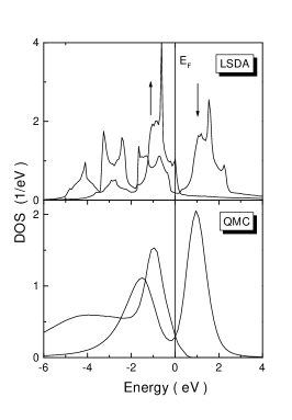
Figure 1: Spin-resolved density of d-states and magnetic moments for ferromagnetic iron in the LSDA and the LDA+QMC calculations for different average Coulomb interactions with J=0.9 eV and temperature T=1500 K.

The QMC method described above is probably the most rigorous real way to solve an effective impurity problem in the framework of DMFT theory. However, it is rather time consuming. Besides that, in the previous section we did not work with complete four-indices Coulomb matrix:

$$\left\langle 12\left|v\right|34\right\rangle=\int d{\bf r}d{\bf r}^{\prime}\psi_{1}^{*}({\bf r})\psi_{2}^{*}({\bf r}^{\prime})v_{scr}\left({\bf{r-r}}^{\prime}\right)\psi_{3}({\bf r})\psi_{4}({\bf r}^{\prime}),$$ (8)

where we define for simplicity $m_{1}\equiv 1$.

For moderately strong correlations (which is the case of iron group metal) one can propose an approximate scheme which is more suitable for the calculations. It is based on the fluctuation exchange (FLEX) approximation by Bickers and Scalapino FLEX generalized to multiband spin-polarized case lda++ ; lda+sp ; mbick . The electronic self-energy in the FLEX is equal to:

$$\Sigma=\Sigma^{HF}+\Sigma^{(2)}+\Sigma^{(ph)}+\Sigma^{(pp)},$$ (9)

where the Hartree-Fock contribution has a standard form:

$$\Sigma_{12,\sigma}^{HF}=\sum_{34}\left[\left\langle 13\left|v\right|24\right\rangle\sum_{\sigma^{\prime}}n_{34}^{\sigma^{\prime}}-\left\langle 13\left|v\right|42\right\rangle n_{34}^{\sigma}\right],$$ (10)

with the occupation matrix $n_{12}^{\sigma}=G_{21}^{\sigma}(\tau\rightarrow-0)$; this contribution to $\Sigma$ is equivalent to spin-polarized “rotationally-invariant” LDA+U method lda+u .

The second-order contribution in the spin-polarized case reads:

$$\Sigma_{12,\sigma}^{(2)}(\tau)=-\sum_{\left\{3-8\right\}}\left\langle 13\left|v\right|74\right\rangle G_{78}^{\sigma}(\tau)*$$ (11)

$$\left[\left\langle 85\left|v\right|26\right\rangle\sum_{\sigma^{\prime}}G_{63}^{\sigma^{\prime}}(\tau)G_{45}^{\sigma^{\prime}}(-\tau)-\left\langle 85\left|v\right|62\right\rangle G_{63}^{\sigma}(\tau)G_{45}^{\sigma}(-\tau)\right],$$ (12)

and the higher-order particle-hole (or particle-particle) contribution

$$\Sigma_{12,\sigma}^{(ph)}\left(\tau\right)=\sum\limits_{34,\sigma^{\prime}}W_{13,42}^{\sigma\sigma^{\prime}}\left(\tau\right)G_{34}^{\sigma^{\prime}}\left(\tau\right),$$ (13)

with p-h (p-p) fluctuation potential matrix:

$$W^{\sigma\sigma^{\prime}}\left(i\omega\right)=\left[\begin{array}[]{cc}W^{\uparrow\uparrow}\left(i\omega\right)&W^{\uparrow\downarrow}\left(i\omega\right)\\ W^{\downarrow\uparrow}\left(i\omega\right)&W^{\downarrow\downarrow}\left(i\omega\right)\end{array}\right],$$ (14)

where the spin-dependent effective potentials has a generalized RPA-form and can be found in lda+sp . Note that for both p-h and p-p channels the effective interactions, according to Eq.(14), are non-diagonal matrices in spin space as in the QMC-scheme, in contrast with any mean-field approximation like LSDA. This can be important for the spin-dependent transport phenomena in transition metal multilayers.

We could further reduce the computational procedure by neglecting dynamical interaction in the p-p channel since the most important fluctuations in itinerant electron magnets are spin-fluctuations in the p-h channel. We take into account static ( of $T$- matrix type) renormalization of effective interactions replacing the bare matrix $U_{12,34}=$ $\left\langle 12\left|v\right|34\right\rangle$ in FLEX-equations with the corresponding spin-dependent scattering $T-$matrix

$$\left\langle 12\left|T^{\sigma\sigma^{\prime}}\right|34\right\rangle=\left\langle 12\left|v\right|34\right\rangle-\sum\limits_{5678}\left\langle 12\left|v\right|56\right\rangle\int\limits_{0}^{\beta}d\tau G_{56}^{\sigma}\left(\tau\right)G_{78}^{\sigma^{\prime}}\left(\tau\right)\left\langle 78\left|T^{\sigma\sigma^{\prime}}\right|34\right\rangle$$ (15)

Similar approximation has been checked for the Hubbard model fleck and appeared to be accurate enough for not too large $U$. Finally, in the spirit of DMFT-approach $\Sigma=\Sigma[G_{0}]$, and all the Green functions in the self-consistent FLEX-equations are in fact the bath Green-functions $G_{0}$.

3 Exchange interactions

An useful scheme for analyses of exchange interactions in the LSDF approach is a so called ”local force theorem”. In this case the calculation of small total energy change reduces to variations of the one-particle density of states MA ; LKG . First of all, let us prove the analog of local force theorem in the LDA++ approach. In contrast with the standard density functional theory, it deals with the real dynamical quasiparticles defined via Green functions for the correlated electrons rather than with Kohn-Sham “quasiparticles” which are, strictly speaking, only auxiliary states for the total energy calculations. Therefore, instead of the working with the thermodynamic potential as a density functional we have to start from the general expression for $\Omega$ in terms of exact Green function in the Table I. We have to keep in mind also Dyson equation $G^{-1}=G_{0}^{-1}-\Sigma$ and the variational identity $\delta\Phi_{LW}=Tr\Sigma\delta G.$ Here $Tr=Tr_{\omega iL\sigma}$ is the sum over Matsubara frequencies $Tr_{\omega}...=T\sum\limits_{\omega}...,$ $\omega=\pi T\left(2n+1\right),$ $n=0,\pm 1,...,$ $T$ is the temperature, and $iL\sigma$ are site numbers ($i$), orbital quantum numbers ($L={l,m}$) and spin projections $\sigma$ , correspondingly. We represent the expression for $\Omega$ as a difference of ”single particle” ($sp$) and ”double counted” ($dc$) terms as it is usual in the density functional theory. When neglecting the quasiparticle damping, $\Omega_{sp}$ will be nothing but the thermodynamic potential of ”free” fermions but with exact quasiparticle energies. Suppose we change the external potential, for example, by small spin rotations. Then the variation of the thermodynamic potential can be written as

$$\delta\Omega=\delta^{*}\Omega_{sp}+\delta_{1}\Omega_{sp}-\delta\Omega_{dc}$$ (16)

where $\delta^{*}$ is the variation without taking into account the change of the ”self-consistent potential” (i.e. self energy) and $\delta_{1}$ is the variation due to this change of $\Sigma$. To avoid a possible misunderstanding, note that we consider the variation of $\Omega$ in the general “non-equilibrium” case when the torques acting on spins are nonzero and therefore $\delta\Omega\neq 0$. In order to study the response of the system to general spin rotations one can consider either variations of the spin directions at the fixed effective fields or, vice versa, rotations of the effective fields, i.e. variations of $\Sigma$, at the fixed magnetic moments. We use the second way. Taking into account the variational property of $\Phi$ one can be easily shown (cf. Ref. luttinger ) that $\delta_{1}\Omega_{sp}=\delta\Omega_{dc}=TrG\delta\Sigma$ and hence

$$\delta\Omega=\delta^{*}\Omega_{sp}=-\delta^{*}Tr\ln\left[\Sigma-G_{0}^{-1}\right]$$ (17)

which is an analog of the ”local force theorem” in the density functional theory LKG .

Further considerations are similar to the corresponding ones in LSDF approach. In the LDA++ scheme, the self energy is local, i.e. is diagonal in site indices. Let us write the spin-matrix structure of the self energy and Green function in the following form

$$\Sigma_{i}=\Sigma_{i}^{c}+{\boldsymbol{\Sigma}}_{i}^{s}{\boldsymbol{\sigma}}\,,\,\,G_{ij}=G_{ij}^{c}+{\bf G}_{ij}^{s}{\boldsymbol{\sigma}}$$ (18)

where $\Sigma_{i}^{\left(c,s\right)}=\frac{1}{2}\left(\Sigma_{i}^{\uparrow}\pm\Sigma_{i}^{\downarrow}\right)$, ${\bf\Sigma}_{i}^{s}=\Sigma_{i}^{s}{\bf e}_{i},$ with ${\bf e}_{i}$ being the unit vector in the direction of effective spin-dependent potential on site $i$, ${\boldsymbol{\sigma}}=(\sigma_{x},\sigma_{y},\sigma_{z})$ are Pauli matrices, $G_{ij}^{c}=\frac{1}{2}Tr_{\sigma}(G_{ij})$ and ${\bf G}_{ij}^{s}=\frac{1}{2}Tr_{\sigma}(G_{ij}{\bf{\sigma}})$. We assume that the bare Green function $G^{0}$ does not depend on spin directions and all the spin-dependent terms including the Hartree-Fock terms are incorporated in the self energy. Spin excitations with low energies are connected with the rotations of vectors ${\bf e}_{i}$: $\delta{\bf e}_{i}=\delta{\boldsymbol{\varphi}}_{i}\times{\bf e}_{i}$ According to the ”local force theorem” (17) the corresponding variation of the thermodynamic potential can be written as $\delta\Omega=\delta^{*}\Omega_{sp}={\bf V}_{i}\delta{\bf\varphi}_{i}$ where the torque is equal to

$${\bf V}_{i}=2Tr_{\omega L}\left[{\boldsymbol{\Sigma}}_{i}^{s}\times{\bf G}_{ii}^{s}\right]$$ (19)

Using the spinor structure of the Dyson equation one can write the Green function in this expression in terms of pair contributions (a similar trick has been proposed in Ref. physica in the framework of LSDF approach). As a result, we represent the total thermodynamic potential of spin rotations or the effective Hamiltonian in the form exchlda

$$\Omega_{spin}=-\sum_{ij}Tr_{\omega L}\left\{\left({\bf G}_{ij}^{s}{\bf\Sigma}_{j}^{s}\right)\left({\bf G}_{ji}^{s}{\boldsymbol{\Sigma}}_{i}^{s}\right)-{\boldsymbol{\Sigma}}_{i}^{s}G_{ij}^{c}{\boldsymbol{\Sigma}}_{j}^{s}G_{ji}^{c}-i\left({\boldsymbol{\Sigma}}_{i}^{s}\times G_{ij}^{c}{\boldsymbol{\Sigma}}_{j}^{s}\right){\bf G}_{ji}^{s}\right\}$$ (20)

one can show by direct calculations that $\left[\frac{\delta\Omega_{spin}}{\delta{\boldsymbol{\varphi}}_{i}}\right]_{G=const}={\bf V}_{i}$ This means that $\Omega_{spin}\left\{{\bf e}_{i}\right\}$ is the effective spin Hamiltonian. The last term in Eq.(20) is nothing but Dzialoshinskii- Moriya interaction term. It is non-zero only in relativistic case where ${\boldsymbol{\Sigma}}_{j}^{s}$ and ${\bf G}_{ji}^{s}$ can be, generally speaking, “non-parallel” and $G_{ij}\neq G_{ji}$ for the crystals without inversion center.

In the nonrelativistic case one can rewrite the spin Hamiltonian for small spin deviations near collinear magnetic structures in the following form $\Omega_{spin}=-\sum_{ij}J_{ij}{\bf e}_{i}{\bf e}_{j}$ where

$$J_{ij}=-Tr_{\omega L}\left(\Sigma_{i}^{s}G_{ij}^{\uparrow}\Sigma_{j}^{s}G_{ji}^{\downarrow}\right)$$ (21)

are the effective exchange parameters. This formula generalize the LSDA expressions of LKG to the case of correlated systems.

Spin wave spectrum in ferromagnets can be considered both directly from the exchange parameters or by the consideration of the energy of corresponding spiral structure (cf. Ref. LKG ). In nonrelativistic case when the anisotropy is absent one has

$$\omega_{{\bf q}}=\frac{4}{M}\sum\limits_{j}J_{0j}\left(1-\cos{\bf qR}_{j}\right)\equiv\frac{4}{M}[J(0)-J({\bf q})]$$ (22)

where $M$ is the magnetic moment (in Bohr magnetons) per magnetic ion.

It should be noted that the expression for spin stiffness tensor $D_{\alpha\beta}$ defined by the relation $\omega_{{\bf q}}=D_{\alpha\beta}q_{\alpha}q_{\beta}$ (${\bf q\rightarrow 0}$) in terms of exchange parameters has to be exact as the consequence of phenomenological Landau- Lifshitz equations which are definitely correct in the long-wavelength limit. Direct calculation basing on variation of the total energy under spiral spin rotations (cf. Ref. LKG ) leads to the following expression

$$D_{\alpha\beta}=-\frac{2}{M}Tr_{\omega L}\sum\limits_{{\bf k}}\left(\Sigma^{s}\frac{\partial G^{\uparrow}\left({\bf k}\right)}{\partial k_{\alpha}}\Sigma^{s}\frac{\partial G^{\downarrow}\left({\bf k}\right)}{\partial k_{\beta}}\right)$$ (23)

were ${\bf k}$ is the quasimomentum and the summation is over the Brillouin zone. The expressions Eqs.(21) and (22) are reminiscent of usual RKKY indirect exchange interactions in the s-d exchange model (with $\Sigma^{s}$ instead of the s-d exchange integral).

We prove in the Appendix that the expression for the stiffness is exact within the local approximation. At the same time, the exchange parameters themselves, generally speaking, differ from the exact response characteristics defined via static susceptibility since the latter contains vertex corrections. The derivation of approximate exchange parameters from the variations of thermodynamic potential can be useful for the estimation of $J_{ij}$ in the different magnetic systems.

4 Computational results

We have started from the spin-polarized LSDA band structure of ferromagnetic iron within the TB-LMTO method OKA in the minimal $s,p,d$ basis set and used numerical orthogonalization to find the $H_{t}$ part of our starting Hamiltonian. We take into account Coulomb interactions only between $d$-states. The correct parameterization of the $H_{U}$ part is indeed a serious problem. For example, first-principle estimations of average Coulomb interactions (U) U ; steiner in iron lead to unreasonably large value of order of 5-6 eV in comparison with experimental values of the U-parameter in the range of 1-2 eV steiner . Semiempirical analysis of the appropriate interaction value oles gives $U\simeq 2.3$ eV. The difficulties with choosing the correct value of $U$ are connected with complicated screening problems, definitions of orthogonal orbitals in the crystal, and contributions of the intersite interactions. In the quasiatomic (spherical) approximation the full $U$-matrix for the $d-$shell is determined by the three parameters $U,J$ and $\delta J$ or equivalently by effective Slater integrals F⁰, F² and F⁴ lda++ ; revU . For example, U= F⁰, J=(F²+F⁴)/14 and we use the simplest way of estimating $\delta J$ or F⁴ keeping the ratio F²/F⁴ equal to its atomic value 0.625 solj .

Note that the value of intra-atomic (Hund) exchange interaction $J$ is not sensitive to the screening and approximately equals to 0.9 eV in different estimations U . For the most important parameter $U$, which defines the bare vertex matrix Eq.(8), we use the value $U=2.3$ eV for Fe oles , $U=3$ eV for Co and Mn and $U=4$ eV for Ni and Cu. To calculate the spectral functions: $A_{\sigma}\left({\mathbf{k}},E\right)=-\frac{1}{\pi}Tr_{L}G_{\sigma}\left({\mathbf{k}},E+i0\right)$ and DOS as their sum over the Brillouin zone we first made analytical continuation for the matrix self-energy from Matsubara frequencies to the real axis using the Pade approximation pade , and then numerically inverted the Green-function matrix as in Eq. (4) for each $\mathbf{k}$-point. In the self-consistent solution of the FLEX equations we used 1024 Matsubara frequencies and the FFT-scheme with the energy cut-off at 100 eV. The sum over irreducible Brillouin zone have been made with 72 k-points for SCF-iterations and with 1661 k-points for the final total density of states.

The depolarization of states near the Fermi level is another important correlation effect. The decrease of the ratio $P=\left[N_{\uparrow}\left(E_{F}\right)-N_{\downarrow}\left(E_{F}\right)\right]/\left[N_{\uparrow}\left(E_{F}\right)+N_{\downarrow}\left(E_{F}\right)\right]$ is a typical sign of spin-polaron effects IKT ; uspekhi . In our approach this effects are taken into account through the $W_{\uparrow\downarrow}^{(ph)}$ terms in the effective spin-polarized LDA++ potential (Eq. (14)).

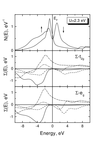
Figure 2: Total spin-polarized density of states and d-part of self-energy for iron with U=2.3 eV and J=0.9 eV for the temperature T=750 K. Two different self-energies for t_2g and e_g d-states in the cubic crystal field symmetry are presented and four different lines corresponds to imaginary part spin-up (full line) and spin-down (dashed line) as well as real part spin-up (dashed-dot line) and spin-down (dashed-double-dot line).

The energy dependence of self-energy in Fig.2 shows characteristic features of moderately correlated systems. At low energies $\left|E\right|<1$ eV we see a typical Fermi-liquid behavior $Im\Sigma\left(E\right)\sim-E^{2},$ $\partial Re\Sigma\left(E\right)/\partial E<0.$ At the same time, for the states beyond this interval within the $d$-bands the damping is rather large (of the order of 1 eV) so these states corresponds to ill-defined quasiparticles, especially for occupied states. This is probably one of the most important conclusions of our calculations. Qualitatively it was already pointed out in Ref. treglia on the basis of a model second-order perturbation theory calculations. We have shown that this is the case of realistic quasiparticle structure of iron with the reasonable value of Coulomb interaction parameter.

Due to noticeable broadening of quasiparticle states the description of the computational results in terms of effective band structure (determined, for example, from the maximum of spectral density) would be incomplete. We present on the Fig.3 the full spectral density $A_{\sigma}\left({\mathbf{k}},E\right)$ including both coherent and incoherent parts as a function of $\mathbf{k}$ and $E$. We see that in general the maxima of the spectral density (dark regions) coincide with the experimentally obtained band structure. However, for occupied majority spin states at about -3 eV the distribution of the spectral density is rather broad and the description of this states in terms of the quasiparticle dispersion is problematic. This conclusion is in complete quantitative agreement with raw experimental data on angle-resolved spin-polarized photoemission kisker with the broad non-dispersive second peak in the spin-up spectral function around -3 eV.

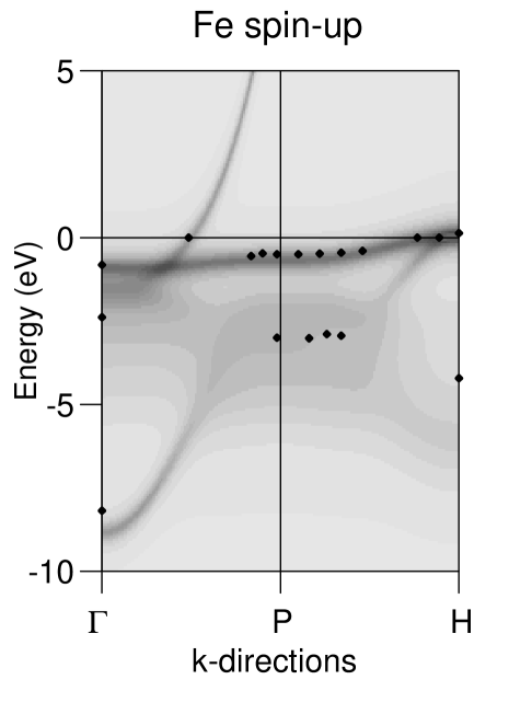
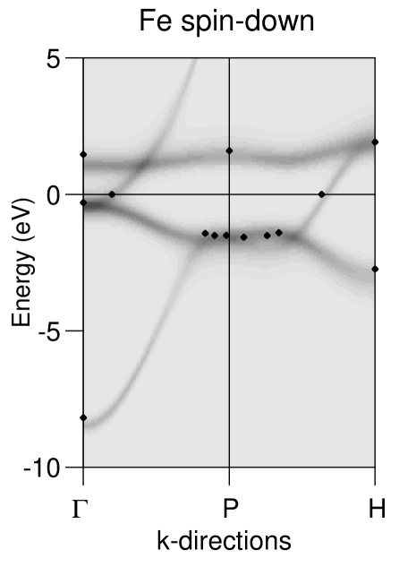
Figure 3: Spectral function of ferromagnetic iron for spin-up (a) and spin-down (b) and the two k-directions in the Brillouin zone compare with the experimental angle resolved photoemission and de Haas - van Alphen (at the E_F=0) points

Comparison of the DOS for transition metals in the Fig. 4 shows an interesting correlations effects. First of all, the most prominent difference from the LSDA calculation is observed for the antiferromagnetic fcc-Mn. There is clear formation of the lower and upper Hubbard bands around $\pm$ 3 eV. Such behavior is related with the half-field Mn d-shell which corresponds to a large phase space for particle-hole fluctuations. For the ferromagnetic bcc-Fe the p-h excitations are suppressed by the large exchange splitting and a bcc structural minimum in the DOS near the Fermi level. In the case of ferromagnetic fcc-Co and Ni the correlation effects are more important then for Fe, since there is no structural bcc-dip in the density of states. One could see a formation of a ”three-peak” structure for the spin-down DOS for Co and Ni and satellite formation around -5 eV. In order to describe the satellite formation more carefully one need to include T-matrix effects liebsch ; drhal or use the QMC scheme in LDA+DMFT calculations. Finally, there is no big correlation effects in non-magnetic fcc-Cu, since the d-states are located well bellow the Fermi level.

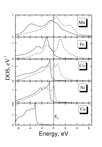
Figure 4: The spin-polarized partial 3d density of states for different transition metals at the temperature T=750 K. The full line is the spin-up DOS and the dashed line is the spin-down DOS.

Using the self-consistent values for $\Sigma_{m}(i\omega)$ computed by QMC technique (Section II) we calculate the exchange interactions (Eq.21) and spin-wave spectrum (Eq.22) using the four-dimensional fast Fourier transform (FFT) method FFT for $({\bf k},i\omega)$ space with the mesh $20^{3}\times 320$. The spin-wave spectrum for ferromagnetic iron is presented in Fig.5 in comparison with the results of LSDA-exchange calculations LKG and with different experimental data omexp1 ; omexp2 ; omexp3 . This room-temperature neutron scattering experiments has a sample dependence (Fe-12%Si in Ref. omexp1 ; omexp3 and Fe-4%Si in Ref. omexp2 ) due to problems with the bcc-Fe crystal growth. Note that for high-energy spin-waves the experimental data omexp3 has large error-bars due to Stoner damping (we show one experimental point with the uncertainties in the $\bf q$ space). On the other hand, the expression of magnon frequency in terms of exchange parameters itself becomes problematic in that region due to breakdown of adiabatic approximation, as it is discussed above. Therefore we think that comparison of theoretical results with experimental spin-wave spectrum for the large energy needs additional investigation of Stoner excitation and required calculations of dynamical susceptibility in the LDA++ approach dinf . Within the LSDA scheme one could use the linear-response formalism Savr to calculate the spin-wave spectrum with the Stoner renormalizations, which should gives in principle the same spin-wave stiffness as our LSDA calculations. Our LSDA spin-wave spectrum agree well with the results of frozen magnon calculations Sandratskii ; Halilov .

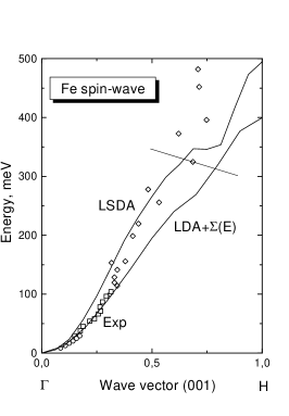
Figure 5: The spin-wave spectrum for ferromagnetic iron in the LSDA and LDA+$\Sigma$ approximations compared with different experiments (circles [16], squares [17], and diamonds [18]) (a); The corresponding spin-wave spectrum from LDA+$\Sigma$ scheme in the (110) plane (b).

At the lower-energy, where the present adiabatic theory is reliable, the LDA++ spin-waves spectrum agree better with the experiments then the result of the LSDA calculations. Experimental value of the spin-wave stiffness D=280 meV/A² omexp2 agrees well with the theoretical LDA++ estimations of 260 meV/A² exchlda .

Appendix

Here we prove that the expression for the stiffness constant Eq.(23) is exact in the framework of DMFT scheme.

A rigorous expression for the stiffness constant has been obtained in Ref. HE :

$$2<S^{z}>D_{\alpha\beta}q_{\alpha}q_{\beta}=C({\bf q})-i{\bf q}\cdot\int\frac{d^{4}k}{(2\pi)^{4}}{\boldsymbol{\gamma}}(k\downarrow,k\uparrow)G_{\downarrow}(k)G_{\uparrow}(k)({\bf v}_{{\bf k}}\cdot{\bf q)}$$ (24)

where

$$C({\bf q})=\frac{1}{2}q_{\alpha}q_{\beta}Tr_{L}\sum_{{\bf k}}\frac{\partial^{2}t({\bf k})}{\partial k_{\alpha}\partial k_{\beta}}(n_{{\bf k}\uparrow}+n_{{\bf k}\downarrow}),$$

$k=({\bf k},k_{0})$ is a momentum-energy 4-vector, $G(k)$ is the electron Green function, $t({\bf k})$ is the one-particle (band) Hamiltonian, $n({\bf k})$ is the one-particle distribution function, ${\boldsymbol{\gamma}}$ is the irreducible vector three-leg vertex. The irreducible scalar and vector vertices, $\gamma$ and ${\boldsymbol{\gamma}}$, are connected with the total ones, $\Gamma_{0}$ and ${\bf\Gamma}$, by Bethe-Salpeter equations and the total vertices satisfy the Ward-Takahashi identity which is the consequence of the rotational invariance. Taking into account the Bethe-Salpeter equations one can rewrite them in terms of the irreducible vertices (for more details, see HE ). Let us assume now that the scalar irreducible vertex $\gamma$ and $\Sigma$ are momentum-independent (which is the real case in DMFT approach). Considering the ${\bf q}$-dependent part of the Ward-Takahashi identity in the limit ${\bf q\longrightarrow 0}$ we have: ${\boldsymbol{\gamma}}(k\downarrow,k\uparrow)=\frac{\partial t({\bf k})}{\partial{\bf k}}\equiv{\bf v}({\bf k}).$ Substituting this into Eq.(24) one has

$$D_{\alpha\beta}=\frac{1}{2<S^{z}>}Tr_{L}\{\sum_{{\bf k}}\frac{\partial^{2}t({\bf k})}{\partial k_{\alpha}\partial k_{\beta}}n_{{\bf k}}-i\int\frac{d^{4}k}{(2\pi)^{4}}v_{{\bf k}\alpha}G_{\downarrow}(k)v_{{\bf k}\beta}G_{\uparrow}(k)\}$$ (25)

On the other hand, our Eq.(22) reads $2<S^{z}>D_{\alpha\beta}=\frac{1}{2}\frac{\partial^{2}J({\bf q})}{\partial q_{\alpha}\partial q_{\beta}}|_{{\bf q}\longrightarrow 0}$ where $J({\bf q})$ is defined by Eq.(21). Calculating the derivatives of the exchange parameters we obtain

$$\frac{\partial J({\bf q})}{\partial q_{\alpha}} = i\int\frac{d^{4}k}{(2\pi)^{4}}Tr_{L}S(k)G_{\downarrow}(k)\frac{\partial t({\bf k})}{\partial k_{\alpha}}G_{\downarrow}(k)S(k)G_{\uparrow}(k+q)$$

(we shift here $k\longrightarrow k+q$ in the integrand). Then

$$\frac{\partial^{2}J({\bf q})}{\partial q_{\alpha}\partial q_{\beta}}|_{{\bf q}\longrightarrow 0}=i\int\frac{d^{4}k}{(2\pi)^{4}}Tr_{L}S(k)G_{\downarrow}(k)\frac{\partial t({\bf k})}{\partial k_{\alpha}}G_{\downarrow}(k)S(k)G_{\uparrow}(k)\frac{\partial t({\bf k})}{\partial k_{\beta}}G_{\uparrow}(k)$$

This expression can be simplified by using the sum rule $(G_{\uparrow}-G_{\downarrow})=G_{\uparrow}SG_{\downarrow}$ (where $S=\Sigma_{\uparrow}-\Sigma_{\downarrow}$) which is the consequence of the Dyson equation provided that only $\Sigma$ is spin-dependent. Taking it into account in Eq.(25) one has

$$\frac{\partial^{2}J({\bf q})}{\partial q_{\alpha}\partial q_{\beta}}|_{{\bf q}\longrightarrow 0}=i\int\frac{d^{4}k}{(2\pi)^{4}}Tr_{L}\{2G_{\uparrow}(k{\bf)}\frac{\partial t({\bf k})}{\partial k_{\alpha}}G_{\downarrow}(k)\frac{\partial t({\bf k})}{\partial k_{\beta}}+\sum_{\sigma}G_{\sigma}^{2}(k{\bf)}\frac{\partial t({\bf k})}{\partial k_{\alpha}}\frac{\partial t({\bf k})}{\partial k_{\beta}}\}$$

The first term is exactly coincide with the last one in Eq.(24) and the first term can be transformed further using the identity: $G_{\sigma}^{2}(k)=\frac{\partial G_{\sigma}(k{\bf)}}{\partial t({\bf k})}$ Then

$$\int\frac{d^{4}k}{(2\pi)^{4}i}\sum_{\sigma}G_{\sigma}^{2}(k{\bf)}\frac{\partial t({\bf k})}{\partial k_{\alpha}}\frac{\partial t({\bf k})}{\partial k_{\beta}}=\sum_{{\bf k}\sigma}\frac{\partial n_{\sigma}({\bf k)}}{\partial t({\bf k})}\frac{\partial t({\bf k})}{\partial k_{\alpha}}\frac{\partial t({\bf k})}{\partial k_{\beta}}$$

Since $n_{\sigma}({\bf k)=}n_{\sigma}[t({\bf k)]}$ we have: $\frac{\partial}{\partial k_{\alpha}}n_{\sigma}[t({\bf k)]=}\frac{\partial n_{\sigma}({\bf k)}}{\partial t({\bf k})}\frac{\partial t({\bf k})}{\partial k_{\alpha}}$ and finally, integrating by part, one obtains:

$$-\sum_{{\bf k}}\frac{\partial n_{\sigma}}{\partial k_{\alpha}}\frac{\partial t({\bf k})}{\partial k_{\beta}}=\sum_{{\bf k}}n_{\sigma}({\bf k)}\frac{\partial^{2}t({\bf k})}{\partial k_{\alpha}\partial k_{\beta}}$$

Thus, our expression (Eq.(23)) coincides with the exact one (Eq.(24)). We use here the only assumption that both the self-energy and three-leg irreducible vertex are momentum independent as well as the Ward-Takahshi identities which are exact consequences of the rotationally invariance of the spin system.

5 Conclusions

We have proposed a general scheme for investigation of the correlation effects in the quasiparticle band structure calculations for itinerant-electron magnets. This approach is based on the combination of the dynamical mean-field theory and the fluctuating exchange approximation. Application of LDA+DMFT method gives an adequate description of the quasiparticle electronic structure for ferromagnetic iron. The main correlation effects in the electron energy spectrum are strong damping of the occupied states below 1 eV from the Fermi level $E_{F}$ and essential depolarization of the states in the vicinity of $E_{F}$. We obtained a reasonable agreement with different experimental spectral data (spin-polarized photo- and thermoemission). The method is rather universal and can be applied for other magnetic systems, both ferro- and antiferromagnets.

We discussed as well a general method for the investigation of magnetic interactions in the correlated electron systems. This scheme is not based on the perturbation theory in “$U$” and could be applied for rare-earth systems where both the effect of the band structure and the multiplet effects are crucial for a rich magnetic phase diagram. Our general expressions are valid in relativistic case and can be used for the calculation of both exchange and Dzialoshinskii- Moriya interactions, and magnetic anisotropy exchlda . An illustrative example of ferromagnetic iron shows that the correlation effects in exchange interactions may be noticeable even in such moderately correlated systems. For rare-earth metals and their compounds, colossal magnetoresistance materials or high-$T_{c}$ systems, this effect may be much more important. For example, the careful investigations of exchange interactions in MnO within the LSDA, LDA+U and optimized potential methods for MnO Sol show the disagreement with experimental spin-wave spectrum (even for small ${\bf q}$), and indicate a possible role of correlation effects.

This work demonstrates an essential difference between spin density functional approach and LDA++ formalism. The latter method deals with the thermodynamic potential as a functional of the local Green function rather than the electron density. Nevertheless, there is a close connection between two techniques (the self-energy corresponds to the exchange- correlation potential, etc). In particular, an analog of local force theorem can be proved for LDA++ approach. It may be useful not only for the calculation of magnetic interactions but also for elastic stresses, in particular, pressure, and other physical properties.

6 Acknowledgments

We are grateful to O.K. Andersen, C. Carbone, P. Fulde, O. Gunnarsson, G. Kotliar, and A. Georges for helpful discussions. The work was supported by the Netherlands Organization for Scientific Research (NWO project 047-008-16) and partially supported by Russian Basic Research Foundation, grant 00-15-96544.

References

- (1) P. Hohenberg and W. Kohn, Phys. Rev. 136, B864 (1964); W. Kohn and L.J. Sham, ibid. 140, A1133 (1965); R. O. Jones and O. Gunnarsson, Rev. Mod. Phys. 61, 689 (1989)
- (2) N.F.Mott, Metal-Insulator Transitions (Taylor and Francis, London 1974)
- (3) K. Terakura, A. R. Williams, T. Oguchi, and J. Kubler, Phys. Rev. Lett. 52, 1830 (1984)
- (4) W. E. Pickett, Rev. Mod. Phys. 61, 433 (1989)
- (5) V. I. Anisimov, F. Aryasetiawan, and A. I. Lichtenstein, J. Phys.: Condens. Matter 9, 767 (1997)
- (6) P. Fulde, J. Keller, and G. Zwicknagl, Solid State Phys.41, 1 (1988)
- (7) D.E. Eastman, F.J. Himpsel, and J.A. Knapp, Phys. Rev. Lett. 44, 95 (1980)
- (8) J. Staunton, B. L. Gyorffy, A. J. Pindor, G. M. Stocks, and H. Winter, J. Phys. F 15, 1387 (1985)
- (9) P. Genoud, A. A. Manuel, E. Walker, and M. Peter, J. Phys.: Cond. Matter 3, 4201 (1991)
- (10) A. Vaterlaus, F. Milani, and F. Meier Phys. Rev. Lett. 65, 3041 (1990)
- (11) R. Monnier, M. M. Steiner, and L. J. Sham, Phys. Rev. B 44, 13678 (1991)
- (12) M. I. Katsnelson and A. I. Lichtenstein, J. Phys.: Cond. Matter 11, 1037 (1999)
- (13) D. Chanderis, J. Lecante, and Y. Petroff, Phys. Rev. B 27, 2630 (1983); A. Gutierez and M. F. Lopez, Phys. Rev. B 56, 1111 (1997)
- (14) R. E. Kirby, B. Kisker, F. K. King, and E. L. Garwin, Solid State Commun. 56, 425 (1985)
- (15) L. Hedin, Phys. Rev. 139, A796 (1965); F. Aryasetiawan and O. Gunnarsson, Rep. Prog. Phys. 61, 237 (1998)
- (16) A. Svane and O. Gunnarsson, Phys. Rev. Lett. 65, 1148 (1990)
- (17) E. K. U. Gross and W. Kohn, Adv. Quant. Chem. 21, 255 (1990)
- (18) A. A. Abrikosov, L. P. Gorkov, and I. E. Dzialoshinskii, Methods of Quantum Field Theory in Statistical Physics (Pergamon Press, New York 1965); G. Mahan, Many-Particle Physics (Plenum Press, New York 1981)
- (19) J. M. Luttinger and J. C. Ward, Phys. Rev. 118, 1417 (1960); see also G. M. Carneiro and C. J. Pethick, Phys. Rev. B 11, 1106 (1975)
- (20) G. Baym and L. P. Kadanoff, Phys. Rev. 124, 289 (1961); G. Baym, Phys. Rev. 127, 1391 (1962)
- (21) T. Jarlborg, Rep. Prog. Phys. 60, 1305 (1997)
- (22) T. Moriya, Spin Fluctuations in Itinerant Electron Magnetism (Springer, Berlin 1985)
- (23) T. Kotani, Phys. Rev. B 50, 14816 (1994); T. Kotani and H. Akai, Phys. Rev. B 54, 16502 (1996); N. E. Zein, V. P. Antropov, and B. N. Harmon, J. Appl. Phys. 87, 5079 (2000)
- (24) D. Ceperley and B. J. Alder, Phys. Rev. Lett. 45, 4264 (1980)
- (25) A. Liebsch, Phys. Rev. Lett. 43, 1431 (1979); Phys. Rev. B 23, 5203 (1981);
- (26) M. M. Steiner, R. C. Albers, and L. J. Sham, Phys. Rev. B 45, 13272 (1992)
- (27) V. Yu. Irkhin, M. I. Katsnelson, and A. V. Trefilov, J. Phys. : Cond. Matter 5, 8763 (1993); S. V. Vonsovsky, M. I. Katsnelson, and A. V. Trefilov, Phys. Metals Metallography 76, 247, 343 (1993)
- (28) T. Greber, T. J. Kreuntz, and J. Osterwalder, Phys. Rev. Lett. 79 ,4465 (1997); B. Sinkovich, L. H. Tjeng, N. B. Brooks, J. B. Goedkoop, R. Hesper, E. Pellegrin, F. M. F. de Groot, S. Altieri, S. L. Hulbert , E. Shekel, and G. A. Sawatzky, Phys. Rev. Lett. 79 3510 (1997)
- (29) G. Treglia, F. Ducastelle, and D. Spanjaard, J. Phys. (Paris) 43 341 (1982)
- (30) V. Drchal, V. Janiš, and J. Kudrnovský in Electron Correlations and Material Properties, edited by A. Gonis, N. Kioussis, and M. Ciftan, Kluwer/Plenum, New York 1999, p. 273.
- (31) J. Igarashi, J. Phys. Soc. Japan 52 , 2827 (1983); F. Manghi, V. Bellini, and C. Arcangelli, Phys. Rev. B 56 7149 (1997)
- (32) W. Nolting, S. Rex, and S. Mathi Jaya, J. Phys. : Cond. Matter 9, 1301 (1987)
- (33) A. I. Lichtenstein and M. I. Katsnelson, Phys. Rev. B 57, 6884 (1998)
- (34) M. I. Katsnelson and A. I. Lichtenstein, Phys. Rev. B 61, 8906 (2000)
- (35) V. I. Anisimov, A. I. Poteryaev, M. A. Korotin, A. O. Anokhin, and G. Kotliar, J. Phys. Cond. Matter 9, 7359 (1997).
- (36) A. I. Liechtenstein, V. I. Anisimov, and J. Zaanen, Phys. Rev. B 52 ,R5467 (1995)
- (37) O.K. Andersen, Phys. Rev. B12, 3060 (1975); O.K. Andersen and O. Jepsen, Phys. Rev. Lett. 53, 2571 (1984)
- (38) A. Georges, G. Kotliar, W. Krauth, and M. Rozenberg, Rev. Mod. Phys. 68, 13 (1996)
- (39) W. Metzner and D. Vollhardt, Phys. Rev. Lett. 62, 324 (1989).
- (40) M. J. Rozenberg, Phys. Rev. B 55, R4855 (1997); K. Takegahara, J. Phys. Soc. Japan 62, 1736 (1992).
- (41) J. E. Hirsch and R. M. Fye, Phys. Rev. Lett. 25, 2521 (1986)
- (42) M. Jarrell and J. E. Gubernatis, Physics Reports 269, 133 (1996)
- (43) N. E. Bickers and D. J. Scalapino, Ann. Phys. (N. Y.) 193, 206 (1989)
- (44) G. Esirgren and N. E. Bickers, Phys. Rev. B 57, 5376 (1998)
- (45) M. Fleck, A. I. Liechtenstein, A. M. Oles, L. Hedin, and V. I. Anisimov, Phys. Rev. Lett. 80, 2393 (1998)
- (46) A. R. Mackintosh, O. K. Andersen, In: Electron at the Fermi Surface, ed.M. Springford (Univ. Press, Cambridge, 1980) p.145
- (47) A. I. Liechtenstein, M. I. Katsnelson, and V. A. Gubanov, J. Phys. F 14, L125; Solid State Commun. 54, 327 (1985); A. I. Liechtenstein, M. I. Katsnelson, V. P. Antropov, and V. A. Gubanov, J. Magn. Magn. Mater. 67, 65 (1987)
- (48) V. P. Antropov, M. I. Katsnelson, and A. I. Liechtenstein, Physica B 237-238, 336 (1997)
- (49) V. I. Anisimov and O. Gunnarsson, Phys. Rev. B 43, 7570 (1991)
- (50) A. M. Oles and G. Stolhoff, Phys. Rev. B 29, 314 (1984)
- (51) V. I. Anisimov, I. V. Solovjev, M. A. Korotin, M. T. Czyzyk, and G. A. Sawatzky, Phys. Rev. B 48, 16929 (1993)
- (52) H. J. Vidberg and J. W. Serene, J. Low Temp. Phys. 29 , 179 (1977)
- (53) V. Yu. Irkhin and M. I. Katsnelson, Physics-Uspekhi 37, 659 (1994)
- (54) E. Kisker, K. Schroeder, T. Gudat, and M. Campagna, Phys. Rev. B 31, 329 (1985)
- (55) S. Goedecker, Comp. Phys. Commun. 76, 294 (1993)
- (56) J. W. Lynn, Phys. Rev. B11, 2624 (1975)
- (57) H. A. Mook and R. M. Nicklow, Phys. Rev. B7, 336 (1973)
- (58) T. G. Peerring, A. T. Boothroyd, D. M. Paul, A. D. Taylor, R. Osborn, R. J. Newport, H. A. Mook, J. Appl. Phys. 69, 6219 (1991)
- (59) S. Y. Savrasov, Phys. Rev. Lett. 81, 2570 (1998)
- (60) L. M. Sandratskii and J. Kübler, J. Phys.: Condens. Matter. 4, 6927 (1992)
- (61) S. V. Halilov, H. Eschrig, A. Y. Perlov, and P. M. Oppeneer, Phys. Rev. B 58, 293 (1998)
- (62) J. A. Hertz and D. M. Edwards, J. Phys. F 3, 2174 (1973)
- (63) I. V. Solovjev and K. Terakura, Phys. Rev. B 58, 15496 ( 1998)