Evidence for softening of first-order transition in $3D$ by quenched disorder

Abstract

We study by extensive Monte Carlo simulations the effect of random bond dilution on the phase transition of the three-dimensional 4-state Potts model which is known to exhibit a strong first-order transition in the pure case. The phase diagram in the dilution-temperature plane is determined from the peaks of the susceptibility for sufficiently large system sizes. In the strongly disordered regime, numerical evidence for softening to a second-order transition induced by randomness is given. Here a large-scale finite-size scaling analysis, made difficult due to strong crossover effects presumably caused by the percolation fixed point, is performed.

The influence of random, confining geometries on first-order phase transitions has been the subject of exciting experimental studies in the past few years. The case of the isotropic to nematic transition of $nCB$ liquid crystals confined into the pores of aerogels consisting of multiply connected internal cavities has been particularly extensively studied and led to spectacular results: The first-order transition of the corresponding bulk liquid crystal is drastically softened in the porous glass and becomes continuous [3], an effect which was not attributed to finite-size effects but rather to the influence of random disorder.

The first attempt to reproduce such a softening scenario using Monte Carlo (MC) simulations was reported by Uzelac et al. [4] who studied a three-dimensional (3D) $q$-state Potts model with spin variables (taking $q=3$ and $4$ states per spin) located inside the randomly connected pores of an aerogel modeled by diffusion-limited cluster aggregation. Although in experimental studies [5] commonly random fields or random uniaxial anisotropies are suggested to explain the softening of the transition, the random disorder chosen in Ref. [4] is coupled to the energy density and thus more akin to bond-dilution.

The qualitative effect of random bond disorder on second-order phase transitions is well understood through the Harris relevance criterion [6], and a beautiful experimental confirmation was reported in a LEED investigation of a two-dimensional (2D) order-disorder transition [7]. For systems with a first-order transition in the pure case, randomness generically softens the transition and, under certain circumstances, may even induce a second-order transition according to a picture first proposed by Imry and Wortis [8].

In 2D, the natural candidate for theoretical investigations is the $q$-state Potts model, since this model is exactly known to exhibit regimes with first- and second-order transitions [9], depending on the value of $q$. Many results were obtained in both regimes in the last ten years [10, 11], including approximate analytic treatments, MC simulations, transfer-matrix calculations, and high-temperature series expansions. Among others also quite intricate problems such as self-averaging and multi-fractality have recently been studied in some detail [11].

In 3D, to date only the Ising model with site dilution has been studied extensively [12]. In accordance with the Harris criterion the presence of random disorder was found to modify the critical exponents to values close to $\nu=0.684(5)$, $\gamma/\nu=1.96(3)$, and $\beta/\nu=0.519(8)$. Concerning the influence of random disorder on first-order transitions, even less is known in 3D. Apart from the exploratory work [13] of Uzelac et al. [4], only the site diluted 3-state Potts model, which in the pure 3D case has a very weak first-order transition [14], has recently been studied via large-scale MC simulations [15]. This study led to the conclusion that the critical exponent $\nu$ governing the scaling behavior of the correlation length is compatible with that of the 3D site diluted Ising model, whereas the $\eta$ exponent is definitely different.

The purpose of this Letter is to present numerical evidence for softening of the transition when it is strongly of first order in the pure system, in order to be sensitive to disorder effects. The paradigm in 3D is the 4-state Potts model, since the correlation length at the transition temperature of the unperturbed system is small enough ($\xi\simeq 3$ in lattice spacing units [16]) to allow simulations of significantly large systems. For the pure 3D 5-state Potts model the first-order transition is already too strong [16]. In the following we, therefore, consider the 4-state bond diluted Potts model on simple-cubic lattices of size $V=L^{3}$ with periodic boundary conditions. The Hamiltonian of the system with independent, quenched random interactions is written as $-\beta{\cal H}=\sum_{(i,j)}K_{ij}\delta_{\sigma_{i},\sigma_{j}}$, where the spins take the values $\sigma_{i}=1,\dots,4$ and the sum goes over all nearest-neighbor pairs $(i,j)$. The coupling strengths are allowed to take two different values $K_{ij}=K\equiv J/k_{B}T$ and $0$ with probabilities $p$ and $1-p$, respectively. The order parameter for a given realization of the $K_{ij}$ is defined by the majority orientation of the spins, $m=\langle\mu\rangle$, where $\mu={(q\rho_{\rm max}-1)}/{(q-1)}$ and $\rho_{\rm max}$ is the maximum value of the density of spins $\rho_{\sigma}$ in the $q=4$ possible spin states. The thermal average over the MC iterations is indicated by brackets $\langle\dots\rangle$, and the physical quantities are then averaged over disorder realizations, e.g., $\bar{m}=\overline{\langle\mu\rangle}$. For each disorder realization the susceptibility is defined as usual via the fluctuation-dissipation theorem, $\chi=KV(\langle\mu^{2}\rangle-\langle\mu\rangle^{2})$.

The present MC simulations consist of two parts. First, a scan of the dilution-temperature plane in order to determine the phase diagram, and second, a large-scale finite-size scaling (FSS) study at $p=0.56$ up to $L=96$ in the dilution regime exhibiting second-order transitions. The spin updates were performed with the cluster-flipping method [17] in the Swendsen-Wang formulation which turned out to be better behaved than the Wolff single-cluster version for high dilutions (small $p$), where small clusters connected by non-vanishing bonds are more likely to appear. We made sure that, by adjusting the length of the runs of cluster algorithms, at least 10 tunnelling events between the two coexisting phases of the pure system ($p=1$) were observed up to lattice size $L=16$. To improve the accuracy, for weak dilutions ($p$ between 1 and 0.68) where we obtained evidence for first-order transitions, we also used multicanonical algorithms [18]. For the determination of the maxima of observables we applied standard histogram reweighting techniques in order to extrapolate the results over a temperature range around the simulation point.

At each probability $p$ and for each realization of the random couplings, between $15\times 10^{3}$ to $30\times 10^{3}$ MC sweeps per spin were performed, resulting in at least 250 (almost) independent measurements of the physical quantities for the largest lattice size considered. This turned out to be sufficient for reliable thermal averages. For the average over disorder realizations, between 2 000 and 5 000 samples were generated.

The phase diagram is determined from the locations of the maxima of the average susceptibility, $K_{\rm max}$, obtained for systems of increasing sizes up to $L=16$. Theoretically we expect that the transition remains of first order in the regime of low impurity concentrations. For increasing concentrations a regime of second-order transitions should appear from a (tri-) critical concentration until the percolation threshold is reached where the transition vanishes altogether. After this percolation threshold, no ordered phase can exist at any finite temperature. Two points are known in the $p-k_{B}T/J$ plane: The transition temperature $T_{t}$ of the pure system [16] $k_{B}T_{t}(p=1)/J\simeq 1.59076$, and $k_{B}T_{t}(p=p_{c})/J=0$ at the percolation threshold $p_{c}\approx 0.2488$. As can be inspected in Fig. 1, the temperatures of the susceptibility maxima for different lattice sizes are very stable and already for $10^{3}$ spins an accurate transition line is obtained. Also shown is the result of a simple mean-field argument taking into account the average number of neighbors, $k_{B}T_{t}(p)/\bar{z}J=\rm const$, where the constant is chosen such that $T_{t}$ of the pure system is reproduced. This leads to a simple linear approximation of the transition line, $k_{B}T_{t}(p)/J=1.59076\times p$, which is surprisingly accurate over a significant range of $p$-values.

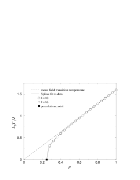
FIG. 1.: Phase diagram of the bond diluted 4-state Potts model in 3D. The solid line is a spline interpolation to guide the eye, and the dashed line shows the transition line within a simple mean-field argument, $T_{t}(p)=pT_{t}(1)$.

By monitoring the FSS behavior of various thermodynamic quantities as well as the (pseudo-) dynamics of the update algorithm, we estimate the tricritical point to be located between $p=0.68$ and $0.84$: The shape of the energy probability densities as well as the Binder cumulants suggest a first-order transition at $p=0.84$ and above while a clear second-order signal is observed at $p=0.68$ and below. For the investigation of the critical properties in the second-order regime we have chosen a dilution $p=0.56$ where the corrections to scaling are seemingly relatively small, since the effective transition temperatures corresponding to the susceptibility maxima remain almost constant in the range of sizes $2\leq L\leq 16$ used for the determination of the phase diagram.

In order to convince ourselves that for $p=0.56$ the transition is indeed of second order, let us first consider the average probability densities of the energy, $P(e)$. In Fig. 2 their shapes close to $K_{\rm max}$ are depicted for various lattice sizes up to $L=96$. We see that the system exhibits for small sizes two distinct peaks which clearly collapse into a single peak when one approaches the thermodynamic limit. This is precisely what is expected at a second-order phase transition, while in the case of a first-order transition the double-peak structure should persist for all sizes and, in fact, should become even more pronounced when the system size increases. Physically, a two-peak structure would reveal the presence of two phases at the transition temperature, and this coexistence is the characteristic feature of a first-order transition. More quantitatively we have confirmed that the effective interface tension $\sigma_{\rm od}$ derived from the usual relation $P_{\rm min}/P_{\rm max}\sim\exp(-2\sigma_{\rm od}(L)L^{d-1})$ vanishes in the infinite-volume limit; see the inset of Fig. 2.

Our final goal is a quantitative characterization of the critical behavior by providing estimates for the critical exponents of the transition. To this end we have performed a standard FSS analysis at $p=0.56$. As can be inspected in Fig. 3, the corrections to asymptotic FSS for $\bar{\chi}_{\rm max}$ seem to become quite small above $L=30$. The data are thus linearly fitted to $a_{\chi}L^{\gamma/\nu}$ for $L$ in the ranges $L_{\rm min}>30$ to $L_{\rm max}=96$, and the resulting exponents are collected in Table I. Selecting the fits with the smallest chi-squared per degree of freedom, $\chi^{2}/{\rm d.o.f}$, we take as the final result the lines in bold face, e.g., $\gamma/\nu=1.50\pm 0.02$.

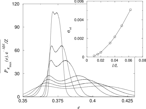
FIG. 2.: The probability density of the energy at $p=0.56$ for sizes $L=16$, 20, 25, 30, 50, 64, and 96, reweighted to the temperature where the two peaks are of equal height. The inset shows the associated effective interface tension.

FIG. 3.: Finite-size scaling behavior of the susceptibility, the magnetization and of $d\ln\bar{m}/dK$ at $K_{\rm max}$ (the quantities have been shifted in the vertical direction for the sake of clarity). The scaling behavior for small lattice sizes is presumably governed by the percolation fixed point, and above a crossover length scale it reaches a new (random) fixed point.

TABLE I.: Linear fits for $\bar{\chi}_{\rm max}$, $(\partial_{K}\ln\bar{m})_{K_{\rm max}}$, and $\bar{m}_{K_{\rm max}}$.

$L_{\rm min}$	$L_{\rm max}$	$\gamma/\nu$	$\chi^{2}/{\rm d.o.f}$
35	96	1.500(14)	0.044
40	96	1.502(17)	0.054
50	96	1.506(27)	0.065
$L_{\rm min}$	$L_{\rm max}$	$1/\nu$	$\chi^{2}/{\rm d.o.f}$
35	96	1.362(13)	1.011
40	96	1.353(16)	0.887
50	96	1.330(25)	0.419
$L_{\rm min}$	$L_{\rm max}$	$\beta/\nu$	$\chi^{2}/{\rm d.o.f}$
35	96	0.592(13)	2.778
40	96	0.608(15)	2.145
50	96	0.645(24)	0.311

The quantity $\partial_{K}\ln\bar{m}$ gives an estimation of the exponent $\nu$, $(\partial_{K}\ln\bar{m})_{K_{\rm max}}\propto L^{1/\nu}$. Here our analysis leads to an estimate of $1/\nu=1.33\pm 0.03$ or $\nu=0.752\pm 0.014$, in agreement with the stability condition of the random fixed point ($\nu\geq 2/D=0.666\dots$) and significantly different from the estimate for the site diluted 3D Ising model ($\nu=0.684(5)$). The same procedure was applied to the magnetization evaluated at the temperature where the susceptibility is maximal. Judging the values of $\chi^{2}/{\rm d.o.f}$ would lead to the result given in bold face in Table I, but the effective exponent for the magnetization is clearly not yet stable. We therefore also considered the FSS behavior of higher (thermal) moments of the magnetization, $\overline{\langle\mu^{n}\rangle}$ which should scale with a dimension $n\beta/\nu$. The results for the first moments exhibit, however, again much stronger corrections to scaling than we observed for $\bar{\chi}$ or $\partial_{K}\ln\bar{m}$, leading to our final estimate of $\beta/\nu=0.65\pm 0.05$. .

From the log-log plots of the three quantities in Fig. 3 one can clearly observe a crossover from a percolation-type behavior at small sizes, characterized by the exponents [19] $\gamma/\nu\simeq 2.05$, $1/\nu\simeq 1.124$, and $\beta/\nu\simeq 0.45$, towards a new regime at large sizes, which presumably corresponds to the random fixed point, with exponents as given above. The numerical evidence for this interpretation is quite striking, but with the present system sizes we can of course not completely rule out the possibility of corrections to scaling, in particular since for the 3D disordered Ising model it is well known that such corrections at the random fixed point are strong (with a correction-to-scaling exponent around $\omega=0.4$). In order to investigate this question for the 3D 4-state Potts model, we tried to fit the physical quantities to the standard expression, e.g., $a_{\chi}L^{\gamma/\nu}[1+b_{\chi}L^{-\omega}+\dots]$, including a sub-dominant correction-to-scaling term. Since 4-parameter non-linear fits are notoriously unstable, we performed linear fits where the exponents are kept fixed and only the amplitudes are free parameters. In Fig. 4, we show a 3D plot of the total $\chi^{2}$ for the susceptibility fits as a function of $\gamma/\nu$ and $\omega$. We observe a clear, stretched valley which confirms that $\gamma/\nu$ is close to $1.5$, but obviously this does not allow any reliable estimation of the correction-to-scaling exponent $\omega$. The same procedure for $1/\nu$ gives qualitatively the same picture and confirms our previous estimate of $1/\nu=1.33$. For $\beta/\nu$, on the other hand, the $\chi^{2}$-landscape turns out to be very flat and extremely sensitive to the fit range.

FIG. 4.: Plot of the $\chi^{2}$ deduced from linear fits of $\bar{\chi}_{\rm max}(L)=a_{\chi}L^{\gamma/\nu}(1+b_{\chi}L^{-\omega})$ in the range $25\leq L\leq 96$. The exponents are fixed parameters and the amplitudes are free. The base plane gives the ranges of variation of the exponents: $1.25\leq\gamma/\nu\leq 1.75$ and $0\leq\omega\leq 5$. A cutoff at $\chi^{2}=50$ has been introduced for clarity of the figure.

To conclude, from large-scale MC simulations of the 3D 4-state bond diluted Potts model we obtained a) the phase diagram in the $p-T$ plane in very good agreement with (rescaled) mean-field theory, b) the approximate location of the tricritical point around $p_{TCP}=0.76(8)$, and c) at the dilution $p=0.56$ clear evidence for softening of the rather strong first-order phase transition in the pure case towards a continuous transition with estimates for the critical exponents of $\nu=0.752(14)$, $\gamma/\nu=1.50(2)$, $\gamma=1.13(4)$, $\beta/\nu=0.65(5)$, and $\beta=0.49(5)$. These are clearly different from the values for both the disordered 3D Ising [$\nu=0.684(5)$, $\gamma/\nu=1.963(5)$] and the $3-$state Potts [$\nu=0.690(5)$, $\gamma/\nu=1.922(4)$] models.

- [1] Unité Mixte de Recherche C.N.R.S. No. 7556.
- [2] Unité Mixte de Recherche C.N.R.S. No. 6634.
- [3] G.S. Iannacchione, G.P. Crawford, S. Žumer, J.W. Doane, and D. Finotello, Phys. Rev. Lett. 71, 2595 (1993).
- [4] K. Uzelac, A. Hasmy, and R. Jullien, Phys. Rev. Lett. 74, 422 (1995).
- [5] X.l. Wu, W.I. Goldburg, M.X. Liu, and J.Z. Xue, Phys. Rev. Lett. 69, 470 (1992); T. Bellini, N.A. Clark, C.D. Muzny, L. Wu, C.W. Garland, D.W. Schaefer, and B.J. Oliver, Phys. Rev. Lett. 69, 788 (1992).
- [6] A.B. Harris, J. Phys. C 7, 1671 (1974).
- [7] L. Schwenger, K. Budde, C. Voges, and H. Pfnür, Phys. Rev. Lett. 73, 296 (1994).
- [8] Y. Imry and M. Wortis, Phys. Rev. B 19, 3580 (1979); M. Aizenman and J. Wehr, Phys. Rev. Lett. 62, 2503 (1989).
- [9] F.Y. Wu, Rev. Mod. Phys. 54, 235 (1982).
- [10] A.W.W. Ludwig, Nucl. Phys. B 285 [FS19], 97 (1987); Nucl. Phys. B 330, 639 (1990); A.W.W. Ludwig and J.L. Cardy, Nucl. Phys. B 330 [FS19], 687 (1987); U. Glaus, J. Phys. A 20, L595 (1987); S. Chen, A.M. Ferrenberg, and D.P. Landau, Phys. Rev. Lett. 69, 1213 (1992); Phys. Rev. E 52, 1377 (1995); Vl. Dotsenko, M. Picco, and P. Pujol, Nucl. Phys. B 455 [FS], 701 (1995); G. Jug and B.N. Shalaev, Phys. Rev. B 54, 3442 (1996); M. Picco, Phys. Rev. Lett. 79, 2998 (1997); J.L. Jacobsen and J.L. Cardy, Nucl. Phys. B 515, 701 (1998); C. Chatelain and B. Berche, Phys. Rev. Lett. 80, 1670 (1998); Nucl. Phys. B 572, 626 (2000); M.A. Lewis, Europhys. Lett. 43, 189 (1998); A. Roder, J. Adler, and W. Janke, Phys. Rev. Lett. 80, 4697 (1998); Physica A 265, 28 (1999); T. Olson and A.P. Young, Phys. Rev. B 60, 3428 (1999).
- [11] B. Derrida, Phys. Rep. 103, 29 (1984), A. Aharony and A.B. Harris, Phys. Rev. Lett. 77, 3700 (1996), S. Wiseman and E. Domany, Phys. Rev. Lett. 81, 22 (1998).
- [12] J.S. Wang and D. Chowdhury, J. Phys. France 50, 2905 (1989), H.O. Heuer, J. Phys. A: Math. Gen. 26, L333 (1993), H.G. Ballesteros, L.A. Fernández, V. Martín-Mayor, A. Muñoz Sudupe, G. Parisi, and J.J. Ruiz-Lorenzo, Phys. Rev. B 58, 2740 (1998), R. Folk, Y. Holovatch, and T. Yavors’kii, Phys. Rev. B 61, 15114 (2000).
- [13] In fact, Ref. [4] was perhaps still too pioneering since, as the authors mention in their paper, no disorder average over the samples was performed.
- [14] W. Janke and R. Villanova, Nucl. Phys. B 489, 679 (1997).
- [15] H.G. Ballesteros, L.A. Fernández, V. Martín-Mayor, A. Muñoz Sudupe, G. Parisi, and J.J. Ruiz-Lorenzo, Phys. Rev. B 61, 3215 (2000).
- [16] W. Janke and S. Kappler, unpublished (1996).
- [17] R.H. Swendsen and J.S. Wang, Phys. Rev. Lett. 58, 86 (1987); U. Wolff, Phys. Rev. Lett. 62, 361 (1989).
- [18] W. Janke, in: Computer Simulation Studies in Condensed Matter Physics VII, eds. D.P. Landau, K.K. Mon, and H.B. Schüttler (Springer Verlag, Berlin, 1994), p. 29.
- [19] C.D. Lorenz and R.M. Ziff, Phys. Rev. E 57, 230 (1998).