Statistical Mechanics of Canonical-Dissipative Systems
and Applications to Swarm Dynamics

Abstract

We develop the theory of canonical-dissipative systems, based on the assumption that both the conservative and the dissipative elements of the dynamics are determined by invariants of motion. In this case, known solutions for conservative systems can be used for an extension of the dynamics, which also includes elements such as the take-up/dissipation of energy. This way, a rather complex dynamics can be mapped to an analytically tractable model, while still covering important features of non-equilibrium systems.

In our paper, this approach is used to derive a rather general swarm model that considers (a) the energetic conditions of swarming, i.e. for active motion, (b) interactions between the particles based on global couplings. We derive analytical expressions for the non-equilibrium velocity distribution and the mean squared displacement of the swarm. Further, we investigate the influence of different global couplings on the overall behavior of the swarm by means of particle-based computer simulations and compare them with the analytical estimations.

I Introduction

The collective motion of biological entities, like schools of fish, flocks of birds, herds of hoof animals, or swarms of insects, recently also attracted the interest of physicists. Here, the question how a long-range order between the moving entities can be established is of particular interest. Consequently, some of the more biologically centered questions of swarming behavior, namely about the resons of swarming or the group size dependence, have been dropped so far in physical swarm models. The main focus was rather on the emergence of coherent motion in a “swarm” of locally or globally coupled particles.

For the coupling different assumptions have been proposed (cf. also Sect. IV), such as the coupling of the particles’ individual orientation (i.e. direction of motion) to the mean orientation of the swarm (czirok-et-96, ; czirok-vicsek-00, ), or the coupling of the particles’ individual position to the mean position (center of mass) of the swarm (mikhailov-zanette-99, ). On the other hand, also some more local couplings have been considered, such as the coupling of the particle’s individual velocity to a local average velocity (toner-tu-95, ; vicsek-et-95, ; czirok-et-99, ; czirok-vicsek-00, ). A different class of models further assumes a local coupling of the particles via a self-consistent field that has been generated by them (lsg-mieth-rose-malch-95, ; lsg-fs-mieth-97, ). This models the case of chemical communication between the particles as widely found in biology. For example, the streaming behaviour of myxobacteria (stevens-95, ; ben-jacob-et-95-b, ; hoefer-et-95, ), or the directed motion of ants (calenbuhr-deneubourg-90, ; edelstein-keshet-94, ; fs-lao-family-97, ) or the coherent movement of cells (schienbein-gruler-95, ) have been described and modeled by means this kind of local coupling.

But long-range or short-range coupling of the particles is only one of the prerequisites that account for swarming. Another one is the active motion of the particles. Of course, particles can also move passively, driven by thermal noise, by convection, currents or by external fields. This kind of driving force however does not allow the particle to change its direction of motion, or velocity etc. itself. Recent models of self-driven particles which are used to simulate swarming behavior vicsek-et-95 ; albano-96 ; helbing-vicsek-99 usually just postulate that the entities move with a certain non-zero velocity, without considering the energetic implications of active motion. In order to do so, we need to consider that the many-particle system is basically an open system which is driven into non-equilibrium.

To this end, our approach to swarming is based on the theory of canonical-dissipative systems. This theory – which is not so well-known even among experts – results from an extension of the statistical physics of Hamiltonian systems to a special type of dissipative systems, the so-called canonical-dissipative systems graham-73 ; haken-73 ; hongler-ryter-78 ; eb-engelh-80 ; eb-81 ; feistel-eb-89 ; eb-00-b . The term dissipative means here that the system is non-conservative and the term canonical means, that the dissipative as well as the conservative parts of the dynamics are both determined by a Hamilton function $H$ (or a larger set of invariants of motion, see Sect. II for details).

This special assumption allows in many cases exact solutions for the distribution functions of many-particle systems, even in far-from-equilibrium situations. This was known already to pioneers as Poincare, Andronov and Bautin who gave exact solutions for a special class of nonlinear oscillators (andronov-witt-chaikin-65, ). In recent work (makarov-eb-velarde-00, ) the properties of canonical-dissipative systems were used to find exact solutions for dissipative solitons in Toda lattices which are pumped with free energy from external sources. The starting point was the well-known Toda theory of soliton solutions in one-dimensional lattices with a special nonlinear potential (exponential for compression and linear for expansion) of the springs toda-81 ; toda-83 , which was then extended towards a non-conservative system graham-73 ; eb-81 ; feistel-eb-89 . In another work eb-00 an application to systems of Fermi and Bose particles was given.

In this paper, we will apply the theory of canonical-dissipative systems to the dynamics of swarms. We start with an outline of the general theory in Sect. II, describing first the deterministic and then the stochastic approach. As a first step towards the dynamics of swarms, in Sect. III we investigate the energetic conditions of swarming, i.e. we discuss the conditions for active motion and their impact on the distribution function and the mean squared displacement of the particles. In Sect. IV we introduce global interactions between the particles which may account for swarming, i.e. for the maintenance of coherent motion of the ensemble. The global interactions are choosen with respect to the general theory of canonical-dissipative systems. By means of computer simulations we show how different kinds of coupling affect the overall behavior of the swarm. In Sect. V we conclude with some ideas how to generalize the approach presented in this paper.

II General Theory of Canonical-Dissipative Systems

II.1 Dynamics of Canonical-Dissipative Systems

Let us consider a mechanical many-particle sytem with $f$ degrees of freedom $i=1,...,f$ and with the Hamiltonian $H(q_{1}\,\ldots\,q_{f},\,p_{1}\,\ldots\,p_{f})$ The corresponding equations of motion are

$$\frac{dq_{i}}{dt}=\frac{\partial H}{\partial p_{i}}\;\;;\quad\frac{dp_{i}}{dt}=-\frac{\partial H}{\partial q_{i}}$$ (1)

Each solution of the system of equations (1)

$$p_{i}=p_{i}(t)\;\;;\quad q_{i}=q_{i}(t)$$ (2)

defines a trajectory on the plane $H=E=$const. This trajectory is determined by the initial conditions, and also the energy $E=H(t=0)$ is fixed due to the initial conditions. We construct now a canonical-dissipative system with the same Hamiltonian, where $g(H)$ denotes the dissipation function:

$$\frac{dp_{i}}{dt}=-\frac{\partial H}{\partial q_{i}}-g(H)\frac{\partial H}{\partial p_{i}}$$ (3)

In order to elucidate this kind of canonical-dissipative dynamics, we will consider different examples for the dissipation function in the following. In general we will only assume that $g(H)$ is a nondecreasing function of the Hamiltonian. The canonical-dissipative system, eq. (3), graham-73 ; eb-81 ; feistel-eb-89 does not conserve the energy because of the following relation:

$$\frac{dH}{dt}=-g(H)\sum_{i}\left(\frac{\partial H}{\partial p_{i}}\right)^{2}$$ (4)

Whether the total energy increases or decreases, consequently depends on the form of the dissipation function $g(H)$. In the simplest case, we may consider a constant friction:

$$g(H)=\gamma_{0}>0$$ (5)

As far as $g(H)$ is always positive, the energy always decays.

In a more interesting case the dissipative function $g(H)$ has a root for a given energy $E_{1}$: $g(E_{1})=0$. Let us further assume that at least in certain neighbourhood of $E_{1}$ the function $g(H)$ is increasing. With these assumptions the states with $H<E_{1}$ are pumped with energy due to the negative dissipation, while energy is extracted from the states with $H>E_{1}$. That means, any given initial state with $H(t=0)<E_{1}$ will increase its energy until it reaches the shell $H(t)=E_{1}$, while any given initial state with $H(t=0)>E_{1}$ will decrease its energy until the shell $H(t)=E_{1}$ is reached, too. Therefore the solution of eq. (4) converges to the energy surface $H=E_{1}$. On this surface the solution of eq. (3) agrees with one of the possible solutions of the original Hamiltonian eq. (1) for $H=E_{1}$.

The simplest ansatz for $g(H)$ with a root $g(H)=0$ is a linear dissipation function:

$$g(H)=C(H-E_{1})$$ (6)

With respect to eq. (4) and the discussion above, it is obvious for this case that the process comes to rest when the shell $H(t)=E_{1}$ is reached. The relaxation time is proportional to the constant $C^{-1}$.

We note that the linear dissipation function eq. (6) has found applications in Toda chains makarov-eb-velarde-00 . Here, the fact that on the shell $H=E_{1}$ the trajectory should obey the original conservative canonical dynamics, has been used to derive exact solutions for canonical-dissipative Toda systems.

A rather general nonlinear and non-decreasing dissipation function, which has been proposed in eb-00 , reads:

$$g(H)=\gamma_{0}-\gamma_{1}\frac{(1+A)}{1+A\exp(\beta H)}$$ (7)

Here $\gamma_{0}>0$ represents the normal positive friction, $\gamma_{1}>0$ represents a kind of negative friction. $A$ is a dimensionless constant and $\beta$ is a parameter with the meaning of a reciprocal temperature. For $\gamma_{1}\leq\gamma_{0}$ the friction is always positive, i.e. energy is extracted. For the opposite case, $\gamma_{1}>\gamma_{0}$, we have negative friction and the system is pumped with energy at least in some parts of the phase space. This allows to drive the system into situations far from equilibrium, therefore in the following we may assume $\gamma_{1}>\gamma_{0}>0$.

In the limit $\beta\rightarrow 0$ and $A\rightarrow 0$ the dissipative function eq. (7) reduces to the linear case, eq. (6), discussed above. On the other hand, for small values of $\beta$ and finite $A$ we get

$$g(H)=\gamma_{0}-\gamma_{1}\frac{(1+A)}{1+A+A\beta H}$$ (8)

which yields $g(H)\to(\gamma_{0}-\gamma_{1})<0$ for $H\to 0$, and $g(H)\to\gamma_{0}$, if $H\to\infty$. This way, the existence of a root $g(E_{1})=0$ is always guaranteed.

Before investigating a special case for $g(H)$ in Sect. III, let us introduce a generalization of the formalism. Instead of a driving function $g(H)$ which depends only on the Hamiltonian we may include the dependence on a larger set of invariants of motion, $I_{0},I_{1},I_{2},...,I_{s}$, for example:

• Hamilton function of the many-particle system: $I_{0}=H$

• total momentum of the many-particle system: ${I}_{1}={P}$

• total angular momentum of the many-particle system: ${I}_{2}={L}$

The dependence on this larger sets of invariants may be considered by defining a dissipative potential $G(I_{0},I_{1},I_{2},...)$. The canonical-dissipation equation of motion, eq. (3) is then generalized towards:

$$\frac{dp_{i}}{dt}=-\frac{\partial H}{\partial q_{i}}-\frac{\partial G(I_{0},I_{1},I_{2},...)}{\partial p_{i}}$$ (9)

Using this generalized canonical-dissipative formalism, by an appropriate choice of the dissipative potential $G$ the system may be driven to particular subspaces of the energy surface, e.g. the total momentum or the angular momentum may be prescribed. Different examples for this will be also discussed in Sect. IV.

II.2 Stochastic Theory of Canonical-Dissipative Systems

We will now investigate an approach to the stationary probabilities which is based on Langevin and Fokker-Planck equations. The Langevin equations are obtained by adding a white noise term $\xi_{i}(t)$ to the deterministic eq. (3):

$$\frac{dp_{i}}{dt}=-\frac{\partial H}{\partial q_{i}}-g(H)\frac{\partial H}{\partial p_{i}}+\Big{(}2D(H)\Big{)}^{1/2}\;\xi_{i}(t)$$ (10)

The essential assumption is that both the strength of the noise, expressed in terms of $D(H)$ and the dissipation, expressed in terms of the friction function $g(H)$ depend only on the Hamiltonian $H$.

With respect to eq. (10), the corresponding Fokker-Planck equation for the probability distribution $\rho(q_{1}...q_{f},p_{1}...p_{f})$ of the many-particle system reads:

$$\frac{\partial\rho}{\partial t}+\sum p_{i}\frac{\partial\rho}{\partial q_{i}}-\sum\frac{\partial H}{\partial p_{i}}\frac{\partial\rho}{\partial p_{i}}=$$

$$\sum\frac{\partial}{\partial p_{i}}\left[g(H)\rho+D(H)\frac{\partial\rho}{\partial p_{i}}\right]$$ (11)

An exact stationary solution of eq. (II.2) reads:

$$\rho^{0}(q_{1}...q_{f},p_{1}...p_{f})=Q^{-1}\;\exp\int\limits_{0}^{H}dH^{\prime}\;\frac{g(H^{\prime})}{D(H^{\prime})}$$ (12)

The derivative of $\rho^{0}$ vanishes if $g(H)=0$, which means that the probability distribution is maximal at the surface $H=E_{1}$.

For the special case of a linear dissipation function, eq. (6), we find the stationary solution:

$$\rho^{0}(q_{1}...q_{f},p_{1}...p_{f})=Q^{-1}\;\exp\left(\frac{cH\;(2E_{1}-H)}{2D}\right)$$ (13)

In the limit of very strong pumping, $H\gg E_{1}$, this probability distribution reduces to a kind of microcanonical ensemble corresponding to the energy $E_{1}$.

The existence of exact solutions for the probability distribution, eq. (12), allows to derive several thermodynamic functions for the many-particle system, such as the mean energy:

$$U=Q^{-1}\int dH\,J(H)\;H\exp\int\limits_{0}^{H}\;dH^{\prime}\;\frac{g(H^{\prime})}{D(H^{\prime})}$$ (14)

where the Jacobian $J(H)$ is defined by:

$$dq_{1}...dq_{f}\;dp_{1}...dp_{f}=J(H)\;dH$$ (15)

The entropy follows from the Gibbs formula which yields here:

$$S=+k_{B}\ln Q-k_{B}\int dH\;J(H)\times$$

$$\times\left[Q^{-1}\exp\int\limits_{0}^{H}\;\frac{g(H)}{D(H)}\right]\;\int\limits_{0}^{H}dH^{\prime}\,\frac{g(H^{\prime})}{D(H^{\prime})}$$ (16)

Further, the system has a Lyapunov functional $K$ which is provided by the Kullback entropy:

$$K[\rho,\rho^{0}]=\int dq_{1}...dq_{f}\,dp_{1}...dp_{f}\;\rho\ln\left(\frac{\rho}{\rho^{0}}\right)$$ (17)

This gives explicitely:

$$K[\rho,\rho_{0}]=\ln Q-\frac{S}{k_{B}}+\left\langle\int\limits_{0}^{H}\frac{g(H)}{D(H)}\right\rangle$$ (18)

This functional is always nonincreasing.

If we want to generalize the description by means of the dissipative potential $G(I_{0},I_{1},I_{2},...)$ as used in eq. (9), the situation is more difficult. But at least if the noise strength $D(H)$ is a constant ($D=$const.), the corresponding Fokker-Planck equation

$$\frac{\partial\rho}{\partial t}+\sum p_{i}\frac{\partial\rho}{\partial q_{i}}-\sum\frac{\partial H}{\partial p_{i}}\frac{\partial\rho}{\partial p_{i}}=$$

$$\sum\frac{\partial}{\partial p_{i}}\left[\frac{\partial G(I_{0},I_{1},I_{2},...)}{\partial p_{i}}\rho+D\frac{\partial\rho}{\partial p_{i}}\right]$$ (19)

is still solvable. Due to the invariant character of the $I_{k}$, the l.h.s. of eq. (II.2) disappears for all functions of $I_{k}$. Therefore we have to search only for a function $G(I_{0},I_{1},I_{2},...)$, for which also the collision term disappears. This way we find the stationary solution of eq. (II.2):

$$\rho^{0}(q_{1}...q_{f},p_{1}...p_{f})=Q^{-1}\;\exp\left(-\frac{G(I_{0},I_{1},I_{2},...)}{D}\right)$$ (20)

The derivative of $\rho_{0}$ vanishes if $G(I_{0},I_{1},I_{2},..)={\rm min.}$ which means that the probability is maximal on the attractor of the dissipative motion.

III Energetic Conditions of Swarming

In this section, we want to apply the general description outlined above to swarm dynamics. Basically, at a certain level of abstraction a swarm can viewed as a many-particle system with some additonal coupling which would account for the typical correlated motion of the entities. In addition, also some energetic conditions must be satisfied in order to keep the swarm moving. Thus, active motion of the particles with a non-zero velocity is another basic ingredient for swarming. Since the conditions for active motion are dropped in many of the currently discussed swarm models albano-96 ; czirok-et-99 ; vicsek-et-95 , we first want to investigate the energetic conditions of swarming, before turning to the second ingredient, coupling of individual motion.

III.1 Conditions for Active Motion

If we omit interactions between the particles, the Hamiltonian of the many-particle system is of the simple form:

$$H=\sum_{i=1}^{N}H_{i}=\sum_{i=1}^{N}\frac{p_{i}^{2}}{2m}$$ (21)

This allows to reduce the description level from the $N$-particle distribution function to the one-particle distribution function:

$$\rho(q_{1}...q_{f},p_{1}...p_{f})=\prod_{i=1}^{N}\rho(\mbox{\boldmath$r_{i}$},\mbox{\boldmath$p_{i}$})$$ (22)

where the variable $\mbox{\boldmath$r$}_{i}$ is now used for the space coordinate of the particle $i$, and $\mbox{\boldmath$p$}_{i}$ stands for the momentum or, if $m=1$ is used in the following, for the velocity of the particle, respectively. The center of mass of the swarm is defined as

$$\mbox{\boldmath$R$}=\frac{1}{N}\sum\mbox{\boldmath$r$}_{i}$$ (23)

whereas the mean momentum $P$ and the mean angular momentum $L$ are defined as:

$$P = \frac{1}{N}\sum\mbox{\boldmath$p$}_{i}$$ (24)

$$L = \frac{1}{N}\sum\mbox{\boldmath$L$}_{i}=\frac{1}{N}\sum\mbox{\boldmath$r$}_{i}\times\mbox{\boldmath$p$}_{i}$$ (25)

With $g(H)=g(p^{2}_{i})$ and $D={\rm const.}$, the Langevin eq. (10) for each particle $i$ reads in the absence of an external potential:

$$\dot{\mbox{\boldmath$r$}_{i}}=\mbox{\boldmath$p$}_{i}\;;\;\;\dot{\mbox{\boldmath$p$}}_{i}=-g(p_{i}^{2})\,\mbox{\boldmath$p$}_{i}+(2\,D)^{1/2}\mbox{\boldmath$\xi$}_{i}(t)$$ (26)

where the strength $D$ of the stochastic force results from the Einstein relation:

$$D=\gamma_{0}k_{B}T$$ (27)

$T$ is the temperature and $k_{B}$ is the Boltzmann constant.

For the dissipation function $g(p^{2})$, we use again the general nonlinear ansatz of eq. (7) in the limit of small values of $\beta$ and finite $A$, eq. (8). By means of the substitutions

$$(1+A)=c\;;\quad\gamma_{1}(1+A)=d_{2}s_{0}\;;\quad\beta A=2d_{2}$$ (28)

and with $H$ of eq. (21), eq. (8) can be written in the form:

$$g(p^{2})=\gamma_{0}-\frac{s_{0}d_{2}}{c+d_{2}p^{2}}$$ (29)

We note that all noninteracting systems with $g=g(p^{2})$ are of canonical-dissipative type.

Eq. (29) agrees with the velocity dependent non-linear friction function previously used in a model of active Brownian particles fs-eb-tilch-98-let ; eb-fs-tilch-99 . These are driven Brownian particles, which move due to the influence of a stochastic force, but additionally are pumped with energy due to a velocity-dependent dissipation function $g(p^{2})$, eq. (29) which is plotted in Fig. 1.

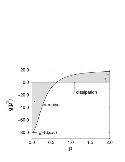
Figure 1: Velocity-dependent dissipation function, $g(p^{2})$, eq. (29) vs. $p$. The velocity ranges for “pumping” ($g(p^{2})<0$) and “dissipation” ($g(p^{2})>0$) are indicated. Parameters: $s_{0}=10.0$, $\gamma_{0}=20.0$, $c=1.0$, $d_{2}=10.0$.

The second term of the r.h.s. in eq. (29) which results from the pumping of energy, has been physically substantiated in our earlier work fs-eb-tilch-98-let ; eb-fs-tilch-99 . We have assumed that the Brownian particles are able to take up energy from the environment at a constant rate $s_{0}$, which can be stored in an internal depot, $e$. The internal energy can be converted into kinetic energy with a velocity dependent rate $d(\mbox{\boldmath$p$})=d_{2}\,p^{2}$, which results in an additional acceleration of the Brownian particle in the direction of movement. The value of the internal energy depot may be further decreased due to internal dissipation processes, described by the constant $c$. Thus the resulting balance equation for the energy depot reads:

$$\frac{de}{dt}=s_{0}-c\,e(t)-d_{2}\,p^{2}\,e(t)$$ (30)

If we assume that the internal energy depot relaxes fast compared to the motion of the particle, we find the quasistationary value:

$$e_{0}=\frac{s_{0}}{c+d_{2}p^{2}}$$ (31)

which eventually leads to the second term of the r.h.s. in eq. (29).

Dependent on the parameters $\gamma_{0}$, $d_{2}$, $s_{0}$, $c$, the dissipation function, eq. (29), may have a zero, where the friction is just compensated by the energy supply. It reads in the considered case:

$$p_{0}^{2}=v_{0}^{2}=\frac{s_{0}}{\gamma_{0}}-\frac{c}{d_{2}}$$ (32)

We see that for $p<p_{0}$, i.e. in the range of small momentums pumping due to negative friction occurs, as an additional source of energy for the Brownian particle. Hence, slow particles are accelerated, while the motion of fast particles is damped.

For $s_{0}d_{2}<\gamma_{0}c$, we find no real-valued root of eq. (32). This is the case of subcritical pumping, where the particle will move more or less like a simple Brownian particle. However, provided the existence of a non-zero momentum $p_{0}$, i.e. for a supercritical pumping, the particle will be able to move in a “high velocity” or active mode tilch-fs-eb-99 ; fs-tilch-eb-00 , which displays several non-trivial features of motion, as will be shown by means of computer simulations in the next section.

III.2 Distribution Function and Dissipative Potential

Due to the pumping mechanism discussed above, the conservation of energy clearly does not hold for the particle, i.e. we now have a non-equilibrium, canonical-dissipative system as discussed in Sect. II. This results in deviations from the known Maxwellian velocity distribution of an equilibrium canonical system.

As pointed out in Sect. II.2, the probability density for the velocity $\rho(\mbox{\boldmath$p$},t)$ obeys the Fokker-Planck eq. (II.2), which reads for the special case of the dissipation function, eq. (29), and in the absence of an external potential:

$$\frac{\partial\rho(\mbox{\boldmath$p$},t)}{\partial t}=\frac{\partial}{\partial\mbox{\boldmath$p$}}\left[\left(\gamma_{0}-\,\frac{d_{2}s_{0}}{c+d_{2}\,p^{2}}\right)\,\mbox{\boldmath$p$}\,\rho(\mbox{\boldmath$p$},t)+D\,\frac{\partial\rho(\mbox{\boldmath$p$},t)}{\partial\mbox{\boldmath$p$}}\right]$$ (33)

We mention that Fokker-Planck equations with nonlinear friction functions are discussed in detail in (klimontovich-95, ).

The stationary solution of eq. (33) is given by eq. (20), which reads in the considered case explicitely:

$$\rho^{0}(\mbox{\boldmath$p$}) = C_{0}\,\exp{\left(-\frac{G_{0}(p^{2})}{D}\right)}$$ (34)

$$= C_{0}\,\left(1+\frac{d_{2}p^{2}}{c}\right)^{\frac{s_{0}}{2D}}\;\exp{\left(-\frac{\gamma_{0}}{2D}\,p^{2}\right)}$$ (35)

where $C_{0}$ results from the normalization condition. $G_{0}(p^{2})$ is the special form of the dissipation potential $G(I_{0},I_{1},I_{2},...)$ considering only $I_{0}=H$ as the invariant of motion, and further $H$ as given by eq. (21). It reads explicitely:

$$G(I_{0})=G_{0}(p^{2})=\gamma_{0}\frac{p^{2}}{2}-\frac{s_{0}}{2}\ln\left(1+\frac{d_{2}p^{2}}{c}\right)$$ (36)

Compared to the Maxwellian velocity distribution of “simple” Brownian particles, a new prefactor appears now in eq. (35) which results from the additional pumping of energy. For a subcritical pumping, $s_{0}d_{2}<c\gamma_{0}$, where we do not find a real-valued root of the dissipation function, eq. (29), only an unimodal velocity distribution results, centered around the maximum $\mbox{\boldmath$p$}_{0}=0$. However, for supercritical pumping, $s_{0}d_{2}>c\gamma_{0}$, if the root of $\gamma(p^{2})$ is real, we find a crater-like velocity distribution, which indicates strong deviations from the Maxwell distribution erdmann-et-00 .

This is also shown in Fig. 2 which presents computer simulations of the velocity distribution of 10.000 particles after a sufficiently long time (only the x-dimension of the 2-d simulation is shown). For the supercritical case, two distinct peaks of the velocity distribution are found at $p_{x}=\{-0.63,+0.63\}$. The values of these maxima agree with the deterministic result for the stationary velocity, eq. (32).

We note that non-Maxwellian velocity distributions for active motion have been also observed experimentally in cells, such as granulocytes franke-gruler-90 ; schienb-gruler-93 .

Figure 2: Velocity distribution $\rho(p_{x})$ for a swarm of $10.000$ particles at $t=1.000$ (i.e. in the stationary regime). Only $p_{x}$ of the 2-d simulation is shown. (top) subcritical pumping $d_{2}=1.0$, (bottom) supercritical pumping, $d_{2}=10.0$. Other parameters: $D=10^{-3}$, $s_{0}=10.0$, $\gamma_{0}=20.0$, $c=1.0$. Initial conditions: $\mbox{\boldmath$r$}_{i}(0)=\{0.0,0.0\}$, $\mbox{\boldmath$p$}_{i}(0)=\{0.0,0.0\}$ for all particles.

III.3 Mean Squared Displacement and Stationary Values

As Fig. 2 shows, the momentum distribution is centered around $\mbox{\boldmath$p$}=0$ both for subcritical and supercritical pumping. If we consider a nearly spherical swarm of particles in the two-dimensional space $\mbox{\boldmath$r$}=\{x,y\}$ as in the computer simulations in this section, its center of mass, eq. (23) and mean momentum, eq. (24) will come to rest. Thus they are not affected by the pumping, but other quantities are, such as the mean squared displacement:

$$\Delta R^{2}(t)=\left\langle\left(\frac{1}{N}\sum\Big{[}\mbox{\boldmath$r$}_{i}(t)-\mbox{\boldmath$r$}_{i}(0)\Big{]}\right)^{2}\right\rangle$$ (37)

In the limit of pure Brownian motion, it is known that the mean squared displacement increases in time as:

$$\Delta R^{2}(t)=4D_{r}t$$ (38)

where $D_{r}=k_{B}T/\gamma_{0}=D/\gamma_{0}^{2}$ is the spatial diffusion coefficient. Thus, eq. (38) will be the lower limit for subcritical pumping of the particles. Contrary, in the case of supercritical pumping it has been shown mikhailov-meinkoehn-97 ; erdmann-et-00 that the mean squared displacement will grow in time approximately as

$$\Delta R^{2}(t)=\frac{2v^{4}_{0}}{D}\,t$$ (39)

where $v_{0}$ is given by eq. (32). Consequently, the diffusion coefficient $D_{r}$ in eq. (38) has for the case of supercritical pumping to be replaced by an effective spatial diffusion coefficient:

$$D_{r}^{\rm eff}=\frac{v_{0}^{4}}{2D}=\frac{1}{2D}\left(\frac{s_{0}}{\gamma_{0}}-\frac{c}{d_{2}}\right)^{2}.$$ (40)

This result holds for noninteracting particles in the limit of relatively weak noise intensity $D$ and/or strong pumping and will therefore give an upper limit for $\Delta R^{2}(t)$. We note the high sensitivity with respect to noise expressed in the scaling with $(1/D)$.

Fig. 3 shows the mean squared displacement of a swarm of 2.000 particles both for the case of sub- and supercritical pumping together with the theoretical results of eqs. (38), (39). We see that for long times the computer simulations for supercritical pumping agree very well with eq. (39).

Figure 3: Mean squared displacement $\Delta R^{2}(t)$, eq. (37) of a swarm of $2.000$ particles as a function of time. (a) supercritical pumping, $d_{2}=10.0$, (b) subcritical pumping, $d_{2}=1.0$. $D=10^{-2}$, for the other parameters and the initial conditions see Fig. 2. The additional curves give the theoretical results of eq. (39) (c) (upper limit) and eq. (38) (d) (lower limit).

Another quantity affected by the sub/supercritical pumping is the stationary velocity $p^{2}_{0}=v^{2}_{0}$, eq. (32). In 2d, these stationary velocities define a cylinder, $p_{x}^{2}+p_{y}^{2}=p_{0}^{2}$, in the four-dimensional state space $\{x,y,p_{x},p_{y}\}$ which attracts all deterministic trajectories of the dynamic system erdmann-et-00 . Fig. 4 shows the results of computer simulations for $p^{2}(t)$ for the case of supercritical pumping. The convergence toward the theoretical result, eq. (32) can be clearly observed.

Figure 4: Averaged squared velocity $p^{2}(t)=1/N\sum p_{i}^{2}(t)$, eq. (26), of a swarm of $2.000$ particles as a function of time. $D=10^{-4}$, for the other parameters and the initial conditions see Fig. 2. The dash-dotted line gives the stationary velocity, eq. (32).

IV Globally Coupled Swarms

So far we have neglected any coupling within the many-particle ensemble. This leads to the effect that the swarm eventually disperses in the course of time, whereas a “real” swarm would maintain its coherent motion. A common way to introduce correlations between the moving particles in physical swarm models is the coupling to a mean value. For example, in (czirok-et-96, ; czirok-vicsek-00, ) the coupling of the particles’ individual orientation (i.e. direction of motion) to the mean orientation of the swarm is discussed. Other versions assume the coupling of the particles’ velocity to a local average velocity, which is calculated over a space interval around the particle czirok-et-99 ; czirok-vicsek-00 .

IV.1 Coupling to the Center of Mass

In this paper, we are mainly interested in global couplings of the swarm, which fit it into the theory of canonical-dissipative systems outlined in Sect. II. As the most simple case we may first discuss the global coupling of the swarm to the center of mass, eq. (23). That means the particle’s position $\mbox{\boldmath$r$}_{i}$ is related to the mean position of the swarm $R$ via a potential $U(\mbox{\boldmath$r$}_{i},\mbox{\boldmath$R$})$. For simplicity, we may assume a parabolic potential:

$$U(\mbox{\boldmath$r$}_{i},\mbox{\boldmath$R$})=\frac{a}{2}\left(\mbox{\boldmath$r$}-\mbox{\boldmath$R$}\right)^{2}$$ (41)

The harmonic potential generates a force directed to the center of mass which can be used to control the dispersion of the swarm. It reads in the considered case:

$$\mbox{\boldmath$\nabla$}U(\mbox{\boldmath$r$})=a\left(\mbox{\boldmath$r$}_{i}-\mbox{\boldmath$R$}\right)=\frac{a}{N}\sum_{j=1}^{N}\left(\mbox{\boldmath$r$}_{i}-\mbox{\boldmath$r$}_{j}\right)$$ (42)

With eq. (42), the corresponding Langevin eq. (26) of the many-particle system reads explicitely:

$$\dot{\mbox{\boldmath$p$}}_{i}=-g(p_{i}^{2})\,\mbox{\boldmath$p$}_{i}-\frac{a}{N}\sum_{j=1}^{N}\left(\mbox{\boldmath$r$}_{i}-\mbox{\boldmath$r$}_{j}\right)+(2\,D)^{1/2}\mbox{\boldmath$\xi$}_{i}(t)$$ (43)

Hence, in addition to the dissipation function there is now an attractive force between each two particles $i$ and $j$ which depends linearly on the distance between them. With respect to the harmonic interaction potential eq. (41), we call such a swarm a harmonic swarm eb-fs-01-pas .

Strictly speaking, the dynamical system of eq. (43) is not a canonical-dissipative one, but as shown in (eb-fs-tilch-99, ) it may be reduced to this type by some approximations, which will be also discussed below. We note that this kind of swarm model has been previously investigated in mikhailov-zanette-99 for the one-dimensional case, however with a different dissipation function $g(p^{2})$, for which we use eq. (29) again. Obviously, as shown in Sect. III.2 swarming will occur only for supercritical conditions.

With the assumed coupling to the center of mass, $R$, the motion of the swarm can be considered as a superposition of two motions: (i) the motion of the center of mass itself, and (ii) the motion of the particles relative to the center of mass. Taking into account that the noise acting on the different particles is not correlated, the center of mass for the assumed coupling obeys a force-free motion,

$$\dot{\mbox{\boldmath$R$}}=\mbox{\boldmath$P$}\;;\;\;\dot{\mbox{\boldmath$P$}}=-\frac{1}{N}\;\sum_{i=1}^{N}g(p_{i}^{2})\,\mbox{\boldmath$p$}_{i}$$ (44)

Because of the nonlinearities in the dissipation function $g(p^{2})$ both motions (i) and (ii) cannot be simply separated. The term $g(p^{2})$ vanishes only for two cases: the trivial one which is free motion without dissipation/pumping, or the case of supercritical pumping where $p_{i}^{2}=p_{0}^{2}$, eq. (32) for each particle. Then, the mean momentum becomes an invariant of motion, $\mbox{\boldmath$P$}(t)=\mbox{\boldmath$P$}_{0}={\rm const.}$ and the center of mass moves according to $\mbox{\boldmath$R$}(t)=\mbox{\boldmath$R$}(0)+\mbox{\boldmath$P$}_{0}(t)$. This behavior may also critically depend on the initial conditions of the particles, $\mbox{\boldmath$p$}_{i}(0)$, and shall be investigated in more detail now.

In mikhailov-zanette-99 an approximation for the mean velocity $\mbox{\boldmath$P$}(t)$ of the swarm in one dimension is discussed which shows the existence of two different asymptotic solutions dependent on the noise intensity $D$ and the initial momentum $\mbox{\boldmath$p$}_{i}(0)$ of the particles. Below a critical noise intensity $D_{c}$, the initial condition $p_{i}^{2}(0)>p_{0}^{2}$ leads to a swarm the center of which travels with a constant non-trivial mean velocity, while for the initial condition $p_{i}^{2}(0)<p_{0}^{2}$ the center of the swarm is at rest.

We can confirm these findings by means of two-dimensional computer simulations presented in Fig. 5 and Fig. 6, which show the mean squared displacement, the average squared velocity of the swarm and the squared mean velocity of the center of mass for the two different initial conditions.

Figure 5: Mean squared displacement $\Delta R^{2}(t)$, eq. (37) of a swarm of $2.000$ particles coupled to the center of mass. Initial conditions: $\mbox{\boldmath$r$}_{i}(0)=\{0.0,0.0\}$, (a) $\mbox{\boldmath$p$}_{i}(0)=\{1.0,1.0\}$, (b) $\mbox{\boldmath$p$}_{i}(0)=\{0.0,0.0\}$, for all particles. Parameters: $a=1$, $D=10^{-8}$, $d_{2}=10.0$, $s_{0}=10.0$, $\gamma_{0}=20.0$, $c=1.0$.

Figure 6: Squared velocity of the center of mass, $P^{2}(t)=\Big{(}N^{-1}\sum_{i}\mbox{\boldmath$p$}_{i}(t)\Big{)}^{2}$ (solid lines) and averaged squared velocity $p^{2}(t)=N^{-1}\sum p_{i}^{2}(t)$ (dashed lines) for the simulations shown in Fig. 5: (top) initial conditions (a), (bottom) initial conditions (b).

For (a) $p_{i}^{2}(0)>p_{0}^{2}$ we find a continuous increase of $\Delta R^{2}(t)$ (Fig. 5 a), while the velocity of the center of mass reaches a constant value: $P^{2}(t)=\Big{(}N^{-1}\sum_{i}\mbox{\boldmath$p$}_{i}(t)\Big{)}^{2}\to p_{0}^{2}$, known as the stationary velocity of the force-free case, eq. (32). The average squared velocity reaches a constant non-trivial value, too, which depends on the noise intensity and the initial conditions, $p_{i}^{2}(0)>p_{0}^{2}$, i.e. on the energy initially supplied (cf Fig. 6 top).

For (b) $p_{i}^{2}(0)<p_{0}^{2}$ we find that the mean squared displacement after a transient time reaches a constant value, i.e. the center of mass comes to rest (Fig. 5 b), which corresponds to $P^{2}(t)\to 0$ in Fig. 6 (bottom). In this case, however, the averaged squared velocity of the swarm reaches the known stationary velocity, $p^{2}(t)=1/N\sum p_{i}^{2}(t)\to p_{0}^{2}$. Consequently, in this case the energy provided by the pumping goes into the motion relative to the center of mass while the motion of the center of mass is damped out (cf. also (eb-fs-01-pas, )). Thus, in the following we want to investigate the relative motion of the particles in more detail.

Using relative coordinates, $\{x_{i},y_{i}\}\equiv\mbox{\boldmath$r$}_{i}-\mbox{\boldmath$R$}$, the dynamics of each particle in the two-dimensional space is described by four coupled first-order differential equations:

$$\dot{x}_{i} = p_{xi}-P_{x}$$

$$\dot{p}_{xi}-\dot{P}_{x} = -g\left(p_{i}^{2}\right)p_{xi}-a\,x_{i}+(2\,D)^{1/2}\xi_{i}(t)$$

$$\dot{y}_{i} = p_{yi}-P_{y}$$

$$\dot{p}_{yi}-\dot{P}_{y} = -g\left(p_{i}^{2}\right)p_{yi}-a\,y_{i}+(2\,D)^{1/2}\xi_{i}(t)$$ (45)

For $\mbox{\boldmath$P$}=0$, i.e. for the initial conditions $p_{i}^{2}<p_{0}^{2}$ and sufficiently long times, this dynamics is equivalent to the motion of free (or uncoupled) particles in a parabolic potential $U(x,y)=a(x^{2}+y^{2})/2$ with the origin $\{0,0\}$. Thus, within this approximation the system becomes a canonical-dissipative system again, in the strict sense used in Sect. II.

Fig. 7 presents computer simulations of eq. (45) for the relative motion of the particle swarm in the parabolic potential. (Note that in this case all particles started from the same position slightly outside the origin of the parabolic potential. This has been chosen in order to make the evolution of the different branches more visible.) As the snapshots of the spatial dispersion of the swarm show, we find after an inital stage the occurence of two branches of the swarm which results from a spontaneous symmetry break (cf. Fig. 7 top). These two branches will after a sufficiently long time move on two limit cycles (as already indicated in Fig. 7 bottom). One of these limit cycles refers to the left-handed, the other one to the right-handed direction of motion in the 2d-space.

Figure 7: Snapshots (relative coordinates) of a swarm of $10.000$ particles moving according to eq. (45) with $\mbox{\boldmath$P$}=0$. (top) $t=15$, (bottom) $t=99$. Initial conditions: $\{x_{i},y_{i}\}=\{0.5,0.0\}$, $\{p_{xi},p_{yi}\}=\{0.0,0.0\}$ for all particles. Parameters: $a=1$, $D=10^{-5}$, $s_{0}=10.0$; $c=1.0$; $\gamma_{0}=20$, $d_{2}=10$.

This finding also agrees with the the theoretical investigations of the deterministic case eb-fs-tilch-99 which showed the existence of a limit cycle with the amplitude

$$r_{0}=\left|p_{0}\right|\,a^{-1/2}$$ (46)

provided the relation $s_{0}d_{2}>\gamma_{0}c$ is fulfilled. In the small noise limit the radius of the limit cycles shown in Fig. 7 agrees with the value of $r_{0}$. Further, Fig. 6 has shown that the averaged squared velocity $p^{2}(t)$ of the swarm indeed approaches the theoretical value of eq. (32).

The existence of two opposite rotational directions of the swarm can be also clearly seen from the distribution of the angular momenta $L_{i}$ of the particles. Fig. 8 shows the existence of a bimodal distribution for $\rho(L)$. (The observant reader may notice that each of these peaks actually consists of two subpeaks resulting from the initial conditions, which are still not forgotten at $t=99$). Each of the main peaks is centered around the theoretical value

$$\left|\mbox{\boldmath$L$}\right|=L_{0}=r_{0}\,p_{0}$$ (47)

where $r_{0}$ is given by eq. (46) and $p_{0}$ is given by eq. (32).

Figure 8: Angular momentum distribution $\rho(L)$ for a swarm of $10.000$ particles at $t=99$. The figure refers to the spatial snapshot of the swarm shown in Fig. 7 (bottom).

The emergence of the two limit cycles means that the dispersion of the swarm is kept within certain spatial boundaries. This occurs after a transient time used to establish the correlation between the individual particles. In the same manner as the motion of the particles becomes correlated, the motion of the center of mass is slowed down until it comes to rest, as already shown in Fig. 6.

This however is not the case if the initial conditions $p_{i}^{2}(0)>p_{0}^{2}$ are chosen. Then, the energy provided by the pumping does not go completely into the relative motion of the particles and the establishment of the limit cycles as discussed above. Instead, the center of mass keeps moving as shown in Fig. 5, while the swarm itself does not establish an internal order. Fig. 9 displays a snapshot of the relative positions of the particles in this case (note the different scales of the axes compared to Fig. 7).

Figure 9: Snapshot (relative coordinates) of a swarm of $10.000$ particles moving according to eq. (45) at $t=99$. Initial conditions: $\{x_{i},y_{i}\}=\{0.5,0.0\}$, $\{p_{xi},p_{yi}\}=\{1.0,1.0\}$ for all particles. Parameters see Fig. 7.

IV.2 Coupling via Mean Momentum and Mean Angular Momentum

In the following we want to discuss two other ways of global coupling of the swarm which fit into the general framework of canonical-dissipative systems outlined in Sect. II. There, we have introduced a dissipative potential $G(I_{0},\mbox{\boldmath$I$}_{1},\mbox{\boldmath$I$}_{2},...)$ which depends on the different invariants of motion, $\mbox{\boldmath$I$}_{i}$. So far, we have only considered $I_{0}=H$, eq. (21) in the swarm model. If we additionally include the mean momentum $\mbox{\boldmath$I$}_{1}=\mbox{\boldmath$P$}$, eq. (24) as the first invariant of motion, the dissipative potential may read:

$$G(I_{0},\mbox{\boldmath$I$}_{1}) = \sum_{i=1}^{N}G_{0}(p_{i}^{2})+G_{1}(\mbox{\boldmath$P$})$$ (48)

$$G_{1}(\mbox{\boldmath$P$}) = \frac{C_{P}}{2}\left(\sum_{i=1}^{N}\mbox{\boldmath$p$}_{i}-N\,\mbox{\boldmath$P_{1}$}\right)^{2}$$ (49)

Here, $G_{0}(p^{2})$ is given by eq. (36). The stationary solution of the probability distribution, $\rho^{0}(\mbox{\boldmath$p$})$ is again given by eq. (20). In the absence of an external potential $U(\mbox{\boldmath$r$})$, the Langevin equation that corresponds to the dissipation potential of eq. (48) reads now:

$$\dot{\mbox{\boldmath$r$}_{i}} = \mbox{\boldmath$p$}_{i}$$

$$\dot{\mbox{\boldmath$p$}}_{i} = -g(p_{i}^{2})\,\mbox{\boldmath$p$}_{i}-C_{P}\left(\sum\mbox{\boldmath$p$}_{i}-N\,\mbox{\boldmath$P_{1}$}\right)$$ (50)

$$+(2\,D)^{1/2}\mbox{\boldmath$\xi$}_{i}(t)$$

The term $G_{1}(\mbox{\boldmath$P$})$ is choosen that way that it may drive the system towards the prescribed momentum $\mbox{\boldmath$P$}_{1}$, where the relaxation time is proportional to $C_{P}^{-1}$. If we would have a vanishing dissipation function, i.e. $g=0$ for $p_{i}^{2}=p_{0}^{2}$, it follows from eq. (IV.2) for the mean momentum:

$$\mbox{\boldmath$P$}(t)=\frac{1}{N}\sum_{i=1}^{N}\mbox{\boldmath$p$}_{i}(t)=\mbox{\boldmath$P$}_{1}+\Big{[}\mbox{\boldmath$P$}(0)-\mbox{\boldmath$P$}_{1}\Big{]}e^{-C_{p}t}$$ (51)

The existence of two terms $G_{0}$ and $G_{1}$ however could lead to competing influences of the resulting forces, and a more complex dynamics of the swarm results. As before, this may also depend on the initial conditions, i.e. $P^{2}_{1}\geq p_{0}^{2}$ or $P^{2}_{1}\leq p_{0}^{2}$.

Fig. 10 shows the squared velocity of the center of mass, $P^{2}(t)$ and the averaged squared velocity of the swarm $p^{2}(t)$ for $P^{2}_{1}\leq p_{0}^{2}$, We find an intermediate stage, where both velocities are equal, before the global coupling drives the mean momentum $P$ towards the prescribed value $\mbox{\boldmath$P$}_{1}$, i.e. $P^{2}(t)\to(P_{1x}^{2}+P_{1y}^{2})$. On the other hand, $p^{2}(t)\to p_{0}^{2}$, as we have found before for the force-free case and for the linearly coupled case for similar initial conditions. The noticeable decrease of $P^{2}$ after the initial time lag can be best understood by looking at the spatial snapshots of the swarm provided in Fig. 11. For $t=10$, we find a rather compact swarm where all particles move into the same (prescribed) direction. For $t=50$, the correlations between the particles have already become effective, which means the swarm begins to establish a circular front, which however does not become a full circle . Eventually, we find again that the energy provided by the pumping goes into the motion of the particles relative to the center of mass, while the motion of the center of mass itself is driven by the prescribed momentum.

Figure 10: Squared velocity of the center of mass, $P^{2}(t)=\Big{(}N^{-1}\sum_{i}\mbox{\boldmath$p$}_{i}(t)\Big{)}^{2}$ (solid lines) and averaged squared velocity $p^{2}(t)=N^{-1}\sum p_{i}^{2}(t)$ (dashed lines) for the simulations shown in Fig. 11.

Figure 11: Snapshots of a swarm of $2.000$ particles moving according to eq. (IV.2). (top) $t=10$, (bottom) $t=50$. Initial conditions: $\{r_{xi},r_{yi}\}=\{0.0,0.0\}$, $\{p_{xi},p_{yi}\}=\{0.0,0.0\}$ for all particles. Parameters: $\{P_{1x},P_{1y}\}=\{0.344,0.344\}$, $C_{p}=10^{-3}$ $D=10^{-8}$, $s_{0}=10.0$; $c=1.0$; $\gamma_{0}=20$, $d_{2}=10$.

For the initial condition $P^{2}_{1}\geq p_{0}^{2}$ the situation is different again, as Fig. 12 shows. Apparently, both curves are the same for a rather small noise intensity, i.e. $P^{2}(t)=p^{2}(t)$ are both equal, but different from $p_{0}^{2}$, eq. (32) and the prescribed momentum $P^{2}_{1}$. This can be only realized if all particles move in parallel into the same direction. Thus, a snapshot of the swarm would much look like the top part of Fig. 11.

Figure 12: Squared velocity of the center of mass, $P^{2}(t)=\Big{(}N^{-1}\sum_{i}\mbox{\boldmath$p$}_{i}(t)\Big{)}^{2}$ (solid lines) and averaged squared velocity $p^{2}(t)=N^{-1}\sum p_{i}^{2}(t)$ (dashed lines) for a swarm of $2.000$ particles moving according to eq. (IV.2). $\{P_{1x},P_{1y}\}=\{1.0,1.0\}$, for the other parameters and initial conditions see Fig. 11.

Eventually, we may also use the second invariant of motion, $\mbox{\boldmath$I$}_{2}=\mbox{\boldmath$L$}$, eq. (25) for a global coupling of the swarm. In this case, the dissipative potential may be defined as follows:

$$G(I_{0},\mbox{\boldmath$I$}_{2}) = \sum_{i=1}^{N}G_{0}(p_{i}^{2})+G_{2}(\mbox{\boldmath$L$})$$ (52)

$$G_{2}(\mbox{\boldmath$L$}) = \frac{C_{L}}{2}\left(\sum\mbox{\boldmath$r$}_{i}\times\mbox{\boldmath$p$}_{i}-N\,\mbox{\boldmath$L_{1}$}\right)^{2}$$ (53)

$G_{0}(p^{2})$ is again given by eq. (36). The term $G_{2}(\mbox{\boldmath$L$})$ shall drive the system to a prescribed angular momentum $\mbox{\boldmath$L$}_{1}$ with a relaxation time proportional to $C_{L}^{-1}$.

$\mbox{\boldmath$L$}_{1}$ can be used to break the symmetry of the swarm towards a prescribed rotational direction. In Sect. IV.1 we have observed the spontaneous occurence of lefthand and righthand rotations of a swarm of linearly coupled particles. Without an additional coupling, both rotational directions are equally probable in the stationary limit. Considering both the parabolic potential $U(\mbox{\boldmath$r$},\mbox{\boldmath$R$})$, eq. (41) and the dissipative potential eq. (52), the corresponding Langevin equation may read now:

$$\dot{\mbox{\boldmath$r$}_{i}} = \mbox{\boldmath$p$}_{i}$$

$$\dot{\mbox{\boldmath$p$}}_{i} = -g(p_{i}^{2})\,\mbox{\boldmath$p$}_{i}-\frac{a}{N}\sum_{j=1}^{N}\left(\mbox{\boldmath$r$}_{i}-\mbox{\boldmath$r$}_{j}\right)$$ (54)

$$+C_{L}\,\mbox{\boldmath$r$}_{i}\times\left(\sum\mbox{\boldmath$r$}_{i}\times\mbox{\boldmath$p$}_{i}-N\,\mbox{\boldmath$L_{1}$}\right)$$

$$+(2\,D)^{1/2}\mbox{\boldmath$\xi$}_{i}(t)$$

The computer simulations shown in Fig. 13 clearly display an unimodal distribution of the angular momenta $L_{i}$ of the particles, which can be compared to Fig. 8 without coupling to the angular momentum. Consequently, we find in the long time limit only one limit cycle corresponding to the movement of the swarm into the same rotational direction. The radius $r_{0}$ of the limit cycle is again given by eq. (46).

Figure 13: Angular momentum distribution $\rho(L)$ for a swarm of $2.000$ particles at $t=99$. For comparison with Fig. 8, the parameters, initial conditions and snapshot times are the same as in Fig. 7. Additional coupling: $C_{L}=0.05,$, $\{L_{1z}\}=\{0.4\}$.

We would like to add that also in this case the dynamics depends on the initial condition, $\mbox{\boldmath$L$}_{1}$. For simplicity, we have assumed here $\left|\mbox{\boldmath$L$}_{1}\right|=L_{0}=r_{0}p_{0}$, eq. (47) which is also reached by the mean angular momentum $L$ in the course of time (cf. Fig. 13). For initial conditions $\left|\mbox{\boldmath$L_{1}$}\right|\ll L_{0}$, there is of course no need for the rotation of all particles into the same direction. Hence we observe both left- and righthanded rotations of the particles with different shares, so that the mean angular momentum is still $\mbox{\boldmath$L$}\to\mbox{\boldmath$L$}_{1}$. This results in a broader distribution of the angular momenta of the particles instead of the clear unimodal distribution shown in Fig. 13. For initial conditions $\left|\mbox{\boldmath$L_{1}$}\right|\gg L_{0}$ on the other hand, the stable rotation of the swarm breaks down after some time, since the driving force $\mbox{\boldmath$L$}\to\mbox{\boldmath$L$}_{1}$ tends to destabilize the attractor $\mbox{\boldmath$L$}\to\mbox{\boldmath$L$}_{0}$. This effect will be investigated in a forthcoming paper, together with some combined effects of the different global couplings.

V Discussion

Eventually, we can also combine the different global couplings discussed above by defining the dissipation potential as:

$$G(I_{0},\mbox{\boldmath$I$}_{1},\mbox{\boldmath$I$}_{2}) = G(p^{2},\mbox{\boldmath$P$},\mbox{\boldmath$L$})$$ (55)

$$= G_{0}(p^{2})+G_{1}(\mbox{\boldmath$P$})+G_{2}(\mbox{\boldmath$L$})$$

$G_{0}(p^{2})$ is given by eq. (36), $G_{1}(\mbox{\boldmath$P$})$ by eq. (49) and $G_{2}(\mbox{\boldmath$L$})$ by eq. (53). Considering further an additional – external or interaction – potential, the corresponding Langevin equation can be written in the more general form:

$$\dot{\mbox{\boldmath$r$}_{i}} = \mbox{\boldmath$p$}_{i}$$

$$\dot{\mbox{\boldmath$p$}}_{i} = -g(p_{i}^{2})\mbox{\boldmath$p$}_{i}-\frac{\partial}{\partial\mbox{\boldmath$r$}_{i}}\left[\alpha_{0}\;U\left(\mbox{\boldmath$r$},\mbox{\boldmath$R$}\right)\right]$$ (56)

$$-\frac{\partial}{\partial\mbox{\boldmath$p$}_{i}}\left[\alpha_{1}\left(\mbox{\boldmath$P$}-\mbox{\boldmath$P_{1}$}\right)^{2}+\alpha_{2}\left(\mbox{\boldmath$L$}-\mbox{\boldmath$L_{1}$}\right)^{2}\right]$$

$$+(2D)^{1/2}\,\mbox{\boldmath$\xi$}_{i}(t)$$

The mean momentum $P$ and mean angular momentum $L$ are given by eqs. (24), (25); whereas the constant vectors $\mbox{\boldmath$P$}_{1}$ and $\mbox{\boldmath$L$}_{1}$ are used to break the spatial or rotational symmetry of the motion toward a preferred direction. The different constants $\alpha_{i}$ may decide whether the respective influence of the conservative or dissipative potential is effective or not, they further determine the time scale when the global coupling becomes effective. The term $g(p^{2})$, eq. (29) on the other hand considers the energetic conditions for the active motion of the swarm, i.e. it determines whether the particle of the swarm are able to “take off” at all.

The combination of the different types of coupling may lead to a rather complex swarm dynamics, as already indicated in the examples discussed in this paper. In particular, we note that the different terms may have competing influences on the swarm, which then would lead to a “frustrated” dynamics with many possible attractors.

In this paper, we have basically restricted the investigation of the swarm dynamics to global couplings which fit into (or can be reduced within some approximations to) the general outline of canonical-dissipative systems. Finally, we want to add some comments on that. On one hand, it is possible to extend this kind of approach also to other invariants of motion, this way e.g. covering previous investigations of swarms coupled via the mean orientation of the particles (czirok-et-96, ; czirok-vicsek-00, ). On the other hand, we want to underline that canonical-dissipative systems are a theoretical class of models, where both conservative and dissipative elements of the dynamics are determined by invariants of the mechanical motion. Thus, from this perspective, a more realistic swarm dynamics may be also based on less restrictive assumptions.

The advantage to use canonical-dissipative systems as a framework for swarm dynamics is given by the fact that in many cases the rather complex dynamics can be mapped to an analytically tractable model. With the Hamiltonian theory of many-particle systems as a starting point, we are able to extend known solutions for conservative systems to non-conservative systems. This allows us to to construct a canonical-dissipative system, the solutions of which converges to the solution of the conservative system with given energy. That means, for given initial conditions, we could predict the asymptotic solution of the canonical-dissipative dynamics by means of the solutions of the Hamiltonian equations on the respective energy surface.

In addition to these theoretical considerations which have a value of their own, we want to note that the framework of canonical-dissipative systems still covers important features of real (biological) systems, such as energy take-up and dissipation. The general description outlined in this paper allows us to gradually add more and more complexity to the swarm model, this way bridging the gap between a known (physical) dynamics to a more complex (biological) dynamics (eb-fs-01-pas, ; eb-fs-01, ). Some hints for this shall be given at the end.

On the level of the “individual” particles, the key dynamics of the model is given by a modified Langevin equation that, in addition to stochastic influences, also considers other forces on the particle, resulting e.g. from external potentials, interactions, use of stored energy (eb-fs-tilch-99, ), or influences of a self-consistent field (lsg-fs-mieth-97, ; lsg-mieth-rose-malch-95, ) that already exceed the framework of canonical-dissipative systems.

The consideration of an external potential also allows to model the spatial environment of the swarm, for instance to consider obstacles (fs-eb-tilch-98-let, ). Additionally, we can also consider that the pumping of energy for the particles is restricted to certain spatial domains which model food sources. In this case the dissipation function $g(H)$ also becomes a spatial function. Such an extension has been already discussed in (steuern-et-94, ; fs-eb-tilch-98-let, ) and can be also implemented in the swarm model discussed here. Eventually, we note that the genuin particle-based approach to collective phenomena used in this paper is not restricted to biological systems, but also applicable for describing and simulating complex interactive systems in a wide range of applications, even in economics and social systems (fs-book-01, ).

- (1) A. Czirok, E. Ben-Jacob, I. Cohen, and T. Vicsek, Physical Review E 54(2), 1791 (1996).
- (2) A. Czirok and T. Vicsek, Physica A 281, 17 (2000).
- (3) A. Mikhailov and D. H. Zanette, Physical Review E 60, 4571 (1999).
- (4) J. Toner and Y. Tu, Physical Review Letters 75(23), 4326 (1995).
- (5) T. Vicsek, A. Czirok, E. Ben-Jacob, I. Cohen, and O. Shochet, Physical Review Letters 75, 1226 (1995).
- (6) A. Czirok, A. L. Barabasi, and T. Vicsek, Physical Review Letters 82(1), 209 (1999).
- (7) L. Schimansky-Geier, M. Mieth, H. Rosé, and H. Malchow, Physics Letters A 207, 140 (1995).
- (8) L. Schimansky-Geier, F. Schweitzer, and M. Mieth, in Self-Organization of Complex Structures: From Individual to Collective Dynamics, edited by F. Schweitzer (Gordon and Breach, London, 1997), pp. 101–118.
- (9) A. Stevens, J. of Biol. Systems 3, 1059 (1995).
- (10) E. Ben-Jacob, . Shochet, I. Cohen, A. Czirok, and T. Vicsek, Physical Review Letters 75/15, 2899 (1995).
- (11) T. Höfer, J. A. Sherratt, and P. K. Maini, Proc. Roy. Soc. London B 259, 249 (1995).
- (12) V. Calenbuhr and J. L. Deneubourg, in Biological Motion, edited by W. Alt and G. Hoffmann (Springer, Berlin, 1990), pp. 453–469.
- (13) L. Edelstein-Keshet, J. Math. Biol. 32, 303 (1994).
- (14) F. Schweitzer, K. Lao, and F. Family, BioSystems 41, 153 (1997).
- (15) M. Schienbein and H. Gruler, Physical Review E 52(4), 4183 (1995).
- (16) E. V. Albano, Physical Review Letters 77(10), 2129 (1996).
- (17) D. Helbing and T. Vicsek, New Journal of Physics 1, 13.1 (1999).
- (18) R. Graham, in Quantum Statistics in Optics and Solid State Physics, edited by G. Höhler (Springer, Berlin, 1973), vol. 66 of Springer Tracts in Modern Physics, pp. 111–???
- (19) H. Haken, Zeitschrift für Physik 273, 267 (1973).
- (20) M. O. Hongler and D. M. Ryter, Zeitschrift für Physik B 31, 333 (1978).
- (21) W. Ebeling and H. Engel-Herbert, Physica A 104, 378 (1980).
- (22) W. Ebeling, in Chaos and Order in Nature, edited by H. Haken (Springer, Berlin, 1981), vol. 11 of Springer Series in Synergetics, pp. 188–???
- (23) R. Feistel and W. Ebeling, Evolution of Complex Systems. Self-Organization, Entropy and Development (Kluwer, Dordrecht, 1989).
- (24) W. Ebeling, in Stochastic Processes in Physics, Chemistry and Biology, edited by J. A. Freund and T. Pöschel (Springer, Berlin, 2000), vol. 557 of Lecture Notes in Physic, pp. 390–399.
- (25) A. A. Andronov, A. A. Witt, and S. Chaikin, Theorie der Schwingungen, vol. I/II (Akademie-Verlag, Berlin, 1965/1969).
- (26) V. Makarov, W. Ebeling, and M. Velarde, Int. J. Bifurc. & Chaos 10(5), 1075 (2000).
- (27) M. Toda, Theory of Nonlinear Lattices (Springer, Berlin, 1981).
- (28) M. Toda, Nonlinear Waves and Solitons (Kluwer, Dordrecht, 1983).
- (29) W. Ebeling, Condensed Matter Physics 3(2), 285 (2000).
- (30) F. Schweitzer, W. Ebeling, and B. Tilch, Physical Review Letters 80/23, 5044 (1998).
- (31) W. Ebeling, F. Schweitzer, and B. Tilch, BioSystems 49, 17 (1999).
- (32) B. Tilch, F. Schweitzer, and W. Ebeling, Physica A 273(3-4), 294 (1999).
- (33) F. Schweitzer, B. Tilch, and W. Ebeling, European Physical Journal B 14(1), 157 (2000).
- (34) Y. L. Klimontovich, Statistical Theory of Open Systems (Kluwer, Dordrecht, 1995).
- (35) U. Erdmann, W. Ebeling, L. Schimansky-Geier, and F. Schweitzer, European Physical Journal B 15(1), 105 (2000).
- (36) K. Franke and H. Gruler, Europ. Biophys. J. 18, 335 (1990).
- (37) M. Schienbein and H. Gruler, Bull. Mathem. Biology 55, 585 (1993).
- (38) A. S. Mikhailov and D. Meinköhn, in Stochastic Dynamics, edited by L. Schimansky-Geier and T. Pöschel (Springer, Berlin, 1997), vol. 484 of Lecture Notes in Physics, pp. 334–345.
- (39) W. Ebeling and F. Schweitzer, Theory in Biosciences (2001), (in press).
- (40) W. Ebeling and F. Schweitzer, in Integrative Systems Approaches to Natural and Social Dynamics – Systems Sciences 2000, edited by M. Matthies, H. Malchow, and J. Kriz (Springer, Berlin, 2001), p. 119-142
- (41) O. Steuernagel, W. Ebeling, and V. Calenbuhr, Chaos, Solitons & Fractals 4, 1917 (1994).
- (42) F. Schweitzer, Brownian Agents and Active Particles, Springer Series in Synergetics (Springer, Berlin, 2002).