Abstract

We present a numerical study of the self-affine profiles obtained from configurations of the $q$-state Potts (with $q=2,3$ and $7$) and $p=10$ clock models as well as from the occupation states for site-percolation on the square lattice. The first and second order static phase transitions of the Potts model are located by a sharp change in the value of the roughness exponent $\alpha$ characterizing those profiles. The low temperature phase of the Potts model corresponds to flat ($\alpha\simeq 1$) profiles, whereas its high temperature phase is associated to rough ($\alpha\simeq 0.5$) ones. For the $p=10$ clock model, in addition to the flat (ferromagnetic) and rough (paramagnetic) profiles, an intermediate rough ($0.5<\alpha<1$) phase - associated to a soft spin-wave one - is observed. Our results for the transition temperatures in the Potts and clock models are in agreement with the static values, showing that this approach is able to detect the phase transitions in these models directly from the spin configurations, without any reference to thermodynamical potentials, order parameters or response functions. Finally, we show that the roughness exponent $\alpha$ is insensitive to geometric critical phenomena.

PACS numbers: 05.10.-a, 05.50.+q, 05.40.-a, 05.70.Fh
Key-words: phase transitions, roughness exponent, lattice spin models
Electronic adressses: redinz@mail.ufv.br; mmartins@mail.ufv.br

I Introduction

In the past decade, the formation of rough surfaces under far-from-equilibrium conditions was a central theme in statistical physics. The application of self-affine fractals and scaling methods was essential to the progress that has been made towards the understanding of these non-equilibrium phenomena. Within this context, the standard tools used to describe various self-affine structures observed in disordered surface growth are the roughness $\alpha$ and the growth $\beta$ exponents [1, 2, 3]. The central goal of this approach is provide information about the correlations between fluctuations of a space and/or time varying property. Theoretical modeling of self-affine growth processes frequently used some of the models investigated in critical phenomena, e.g., directed percolation, random field Ising [1] and sine-Gordon models [4]. These efforts faced an old problem: thirty years after the renormalization group theory of critical phenomena, the quantitatively accurate prediction of the location and characteristics of phase transitions still constitute a challenging and controversial question [5]. This is particularly true when one considers systems with random quenched disorder (e.g., random field Ising and Potts models, spin glasses and structural glasses [6]), which exhibit non-trivial features such as extremely slow dynamics, aging, ergodicity breaking, complex energy landscapes, etc.

On the other hand, the inverse problem, i.e., using the roughness exponents to study the main features of the phase diagram of equilibrium spin models, has not been much explored up to now. In 1997, de Sales et al. [7] mapped cellular automata (CA) configurations on solid-on-solid like profiles and used the roughness exponent $\alpha$ to classify the elementary Wolfram CA rules. Later, they also shown that this exponent can be used to detect the frozen-active transition in the one dimensional Domany-Kinzel CA (DKCA) [8] without any reference to order parameters or response functions. As we mentioned before, beyond the roughness exponent $\alpha$, the growth exponent $\beta$ is another critical index used to describe roughening processes in the surface growth context. Recently, Atman and Moreira [9] determined the exponent $\beta$ for the growth process generated by the spatiotemporal patterns of the DKCA. The value of $\beta$ exhibits a cusp at the frozen-active frontier and, if one observes the difference configuration between two DKCA replicas, also at the active-chaotic critical frontier. The advantage of this method to find the phase diagram of the DKCA is that it is not necessary to wait for the system “thermalizes”, a process which often dispends a lot of computational time.

In this paper we extended the roughness exponent analysis to other standard models of statistical mechanics. Specifically, we study the $q$-state Potts model (with $q=2,3$ and $7$), the simplest locally interacting statistical model exhibiting both first and second order static phase transitions. We study also the $p=10$ clock model for which a Kosterlitz-Thouless type phase transition is observed. Finally, since any connectivity problem can be studied by starting with pure random percolation and then adding interactions, we apply the roughness method to random-site percolation.

In section 2 we describe the models and define the mapping between spin configurations and walk profiles. In section 3, using the mapping between spin states and profiles, we characterize the phases of the random-site percolation problem, Potts and clock models by the roughness exponent $\alpha$. Finally, we conclude and indicate future directions of this work in section 4.

II Models and Formalism

The $q$-state Potts ferromagnet consists of spin variables $\sigma_{i}$ which may take on $q$ discrete values $\sigma_{i}=0,1,\ldots,(q-1)$ and are coupled by the dimensionless Hamiltonian

$$-\beta{\cal H}=K\sum_{\langle ij\rangle}\delta(\sigma_{i},\sigma_{j})\;\;\;\;\;\;,$$ (1)

where $\delta(,)$ is the Kronecker delta function.

The $p$-state clock model is defined by the Hamiltonian

$$-\beta{\cal H}=K\sum_{\langle ij\rangle}\cos\left\{\frac{2\pi}{p}(\sigma_{i}-\sigma_{j})\right\}\;\;\;\;\;\;,$$ (2)

in which each spin can assume $p$ discrete values $\sigma_{i}=0,1,\ldots,p-1$.

In Eqs. (1) and (2) the sums in $\langle ij\rangle$ runs over the lattice sites and their nearest-neighbors, $\beta=1/k_{B}T$, $T$ is the temperature, $K=\beta J$ and $J>0$ is the coupling constant. We simulated the Potts model with $q=2,3$ and $7$ and the clock model with $p=10$ states, on square lattices of $N=L\times L$ sites imposing periodic boundary conditions. For updating the spins we use a sequential Monte Carlo heat-bath process.

In random-site percolation, one randomly occupies a fraction $p$ of the sites of a $d$-dimensional lattice ($\sigma_{i}=0$: empty site; $\sigma_{i}=1$: occupied site). When $p$ is small, the pair connectedness length scale $\xi_{p}$ is short, comparable to the lattice constant $a$. However, when $p$ approaches $p_{c}$, there occur fluctuations in the characteristic size of clusters on all scales from $a$ to $\xi_{p}$, which diverges as $\xi_{p}\sim|p-p_{c}|^{-\nu_{p}}$. Each feature of thermal critical phenomena has a corresponding analog in percolation, so that the percolation problem is called a geometric or connectivity critical phenomena. For site percolation on the square lattice the critical probability is $p_{c}=0.59275\pm 0.00003$ [10].

In the present work we mainly focused on the numerical study of the self-affine profiles generated from the configurations in the ordered and disordered phases of the Potts and clock models and in the site-percolation problem. As shown in a previous work  [8] the spin states can be mapped on random walk-like profiles and the correlations present in them can be measured using the roughness exponent. The simplest method to generate walk profiles from the spin configurations at a time $t$ is a 1:1 mapping in which each spin state $\sigma_{i}(t)$ is associated to a step (to the right or to the left) of a one-dimensional walk. Specifically, to an unique spin configuration $\{\sigma_{1}(t),\sigma_{2}(t),\ldots,\sigma_{N}(t)\}$ corresponds a spatial profile $\{h_{1}(t),h_{2}(t),\ldots,h_{N}(t)\}$, given by the sequence of the walker displacements $h_{i}$ after $i$ unit steps defined as

$$h_{i}(t)=\sum_{j=1}^{i}\rho_{j}(t)\;\;\;\;\;\;,$$ (3)

where $\rho_{j}=\sigma_{j}-(q-1)/2$ for the $q=3$ and $q=7$ Potts models, $\rho_{j}=\sigma_{j}-5$ ($\rho_{j}=\sigma_{j}-4$) if $\sigma_{j}\leq 4$ (if $\sigma_{j}>4$) for the $p=10$ clock model, and $\rho_{j}=2\sigma_{j}-1$ for the Ising ($q=2$) model and site-percolation.

After obtained the profiles by this mappings, the roughness exponent $\alpha$ was calculated by determining the average standard deviation of parts of the profiles with various scales $\epsilon$. At site $i$, in the scale $\epsilon$, the rms displacement fluctuation is given by:

$$w_{i}(N,\epsilon,t)=\sqrt{\frac{1}{2\epsilon+1}\sum_{j=i-\epsilon}^{i+\epsilon}(h_{j}(t)-\overline{h}_{i}(t))^{2}}\;\;\;\;\;\;,$$ (4)

with

$$\overline{h}_{i}(t)=\frac{1}{2\epsilon+1}\sum_{j=i-\epsilon}^{i+\epsilon}h_{j}(t)\;\;\;\;\;\;.$$ (5)

The roughness in the scale $\epsilon$ is given by

$$W(N,\epsilon,t)=\frac{1}{N}\sum_{i=1}^{N}w_{i}(N,\epsilon,t)\;\;\;\;\;\;.$$ (6)

The roughness $W(\epsilon)$ can distinguish two possible types of profiles. If it is random or even exhibits a finite correlation length extending up to a characteristic range (such as in a Markov chain), then $W\sim\epsilon^{1/2}$ as in a normal random walk. In contrast, if the profile has infinitely long-range correlations (no characteristic length), then its roughness will be described by a power law scaling such as

$$W(\epsilon)\sim\epsilon^{\alpha}\;\;\;\;\;\;,$$ (7)

with $\alpha\neq 1/2$. The case $\alpha>1/2$ implies that the profile presents persistent correlations, i.e., a given displacement sequence (increasing or decreasing) is likely to be close to another of the same type. On the other hand, profiles with $\alpha<1/2$ are anticorrelated, which means that displacement sequences containing a great fraction of steps to the right are more likely to alternate with another one in which steps to the left are predominant and vice versa. The exponent $\alpha$ is restricted to the interval $[0,1]$ and is related to the fractal dimension $d$ of the profile by $\alpha=2-d$ [1, 2].

III Results

Before discuss the results, we shall make a very brief review of the equilibrium phase diagrams of the $q$-state Potts and $p=10$ clock models. The square lattice $q$-state Potts ferromagnet presents a second order phase transition for $q<5$ and a first order one for $q\geq 5$ at the critical temperatures $T_{c}^{(q)}=1/\ln(1+\sqrt{q})$ (in units of $J/k_{B}$). The $p$-state clock model interpolates between the Ising ($p=2$) and the XY ($p\rightarrow\infty$) models. For $p\geq 5$ one expects the emergence of a soft spin-wave phase between the ordered, low temperature, and the disordered, high temperature phases [11]. For the $p=10$ case, the spin-wave phase is limited by the transition temperatures $T_{Ac}^{(p=10)}\simeq 0.24$ and $T_{Bc}^{(p=10)}\simeq 1.0$ [12] .

In Fig. 1 we show typical walk profiles generated by spin configurations of the Ising model ($q=2$). From data similar to those in Fig. 1 for different temperatures, we obtained the behavior of the roughness exponents $\alpha$ as shown in Fig. 2, for the Ising model with $L=64$ and 128. These results correspond to averages over typically $M=100$ random initial configurations taken after thermalization. The roughness exponent exhibits an abrupt fall from $\alpha\simeq 1.0$ to $\alpha\simeq 0.5$ at the temperature $T_{q=2}\simeq 1.13$ which agrees with the static critical value $T_{c}^{(q=2)}=1.134...$ As we increase the system size we can note that the change of $\alpha$ at $T_{q=2}$ becomes sharper, suggesting a step function for the $\alpha(T)$ curve at the thermodynamical limit, and a high-temperature value of the exponent $\alpha$ tending to $\alpha=0.5$. Indeed, the inset in Fig. 2 shows that the width $\Delta T=T_{1}-T_{2}$ goes to zero as $N$ increases, where $\Delta T$ is arbitrarily defined as the difference between the observed upper temperature $T_{1}$ for which $\alpha\simeq 0.999$ and the temperature $T_{2}$ for which $\alpha$ has fallen to half its maximum ($\alpha\simeq 0.75$). We also observe that, in this same limit, the temperature $T_{1}$ tends to the exact critical temperature $T_{c}^{(q=2)}$ ($T_{1}(L=64)=1.075$, $T_{1}(L=128)=1.10$ and $T_{1}(L=256)=1.125$).

In Fig. 3 we show similar behaviors for the $q=3$ and $q=7$ Potts model with $L=128$. The abrupt falls in the exponent $\alpha$ are located at the temperatures $T_{q=3}\simeq 0.99$ and $T_{q=7}\simeq 0.77$ which are also in good agreement with the static critical values $T_{c}^{(q=3)}=0.994...$ and $T_{c}^{(q=7)}=0.773...$ The values $\alpha\simeq 1$ observed in the low temperature phases correspond to flat profiles reflecting the existence of long-range order (magnetization). In contrast, the values $\alpha\simeq 0.5$ obtained in the high temperature phases characterize random walk profiles, as expected for disordered spin configurations. Finally, any qualitative difference is observed among the $\alpha(T)$ curves across the critical surfaces corresponding to second ($q=3$) or first ($q=7$) order phase transitions.

In Fig. 4 we show a typical log-log plot of $W\times\epsilon$ for the Ising model, whose fitted slopes give the roughness exponent values. We observe, in general, the existence of two distinct linear portions in the curve, whose intersection point defines a particular length scale $\epsilon^{*}$. The value of $\epsilon^{*}$ seems to be a measure of the average size of the spin islands or magnetized micro-domains limited by the correlation length $\xi(T)$. Indeed, at the ferromagnetic phase, for small scales ($\epsilon<\epsilon^{*}$) there is resolution to see the local spin fluctuations around the smooth profile, which leads to $0.5<\alpha<1.0$. For large scales ($\epsilon>\epsilon^{*}$) the profile is flat and the values $\alpha\simeq 1$ reflect the long-range order. At high temperatures $\epsilon^{*}$ rapidly decreases to the lattice constant $a=1$, which agrees with the fact that such crossover is not observed in a random profile. An additional support to the relationship between $\epsilon^{*}$ and $\xi$ is provided by Fig. 5 which shows that $\epsilon^{*}$ (for the Ising model) has a peak near the temperature $T_{q=2}$. The height and sharpness of this peak increase with the system size. A finite size analysis for the Ising model shows that the maximum value of the crossover length $\epsilon^{*}$ (which occurs near the critical point) scales linearly with the system size $N=L^{2}$, similarly to the correlation length $\xi$. In fact, Fig. 5 suggests that $\epsilon^{*}$ diverges at $T_{c}$ as $\epsilon^{*}\sim(T-T_{c})^{-\mu}$ for the Ising model. Moreover, the behavior of $\epsilon^{*}$ near $T_{c}^{(q=2)}$ is similar to the $2D$ Ising model correlation length, whose exact expression $\xi=1/(\beta^{*}-\beta)$ is known for $\beta<\beta_{c}$ [13] (see Fig. 5). Here, the dual inverse temperature $\beta^{*}$ is given by $(e^{\beta}-1)\times(e^{\beta^{*}}-1)=2$.

A recent work by Kantelhardt et al. [14] provides the strongest support to the close relation between the length scales $\epsilon^{*}$ and $\xi$ that we suggest here based on our limited numerical evidence. These authors demonstrated that the detrended fluctuation analysis (DFA), which we used here in zero-order, can detect crossovers in the observed long-range correlation behavior of data series. They analyzed artificial data with a crossover from long-range correlations ($\alpha>0.5$) for $s<s_{x}$ to uncorrelated behavior for $s>s_{x}$ or vice-versa. Their DFA results clearly revealed the crossover and provided estimated crossover lengths $s_{x}^{(n)}$ always larger than the real $s_{x}$ by a systematic deviation which increases with the detrending order $n$. Also, the estimated $s_{x}^{(n)}$ were less accurate for $\alpha$ close to $0.5$. The support for our suggestion comes from the analogy between the artificial series generated by Fourier transforms studied in [14] and our data series build from spin configurations in which only thermal correlations, extending up to the scale $\xi$ (the correlation length), are present.

The existence of two distinct linear portions in the plots of $W\times\epsilon$ is also observed in the Potts model. In Fig. 6 it is shown the behavior of $\epsilon^{*}$ as function of temperature for the Potts model with $q=3$ and 7. We can note the sharp peaks around the temperatures $T_{c}^{(q=3)}$ and $T_{c}^{(q=7)}$.

In Fig. 7 we show typical walk profiles generated by spin configurations of the $p=10$ clock model at three temperatures: $T=0.15$, located in the ordered phase, $T=0.40$, in the spin-wave phase and $T=1.60$ in the disordered one. The roughness exponent $\alpha$ as a function of the temperature for the $p=10$ clock model is shown in Fig. 8. It suggests the existence of three distinct phases, namely, a low temperature flat ($\alpha\simeq 1$) phase with long-range order and extending up to $T_{A\;p=10}\simeq 0.25$, a high temperature, disordered and rough ($\alpha\simeq 0.5$) phase for $T>T_{B\;p=10}\simeq 1.0$, and an intermediate, rough ($0.80<\alpha<0.90$) phase on the temperature range $T_{A\;p=10}<T<T_{B\;p=10}$. These transition temperatures are in good agreement with those obtained for the static transitions between the ferromagnetic, paramagnetic and soft spin-wave phases of this model [12]. The behavior of $\epsilon^{*}$ as a function of temperature is shown in Fig. 9. $\epsilon^{*}(T)$ exhibits a sharp peak around $T_{B\;p=10}$, the critical temperature separating the paramagnetic and the spin-wave phases, as well as a sudden jump near $T_{A\;p=10}$, where the transition between the ferromagnetic and spin-wave phase occurs. But, the main feature of Fig. 9 is that, in the spin-wave phase ($T_{A\;p=10}<T<T_{B\;p=10}$), $\epsilon^{*}$ has a high and almost constant value as expected for a Kosterlitz-Thouless “critical” phase characterized by an infinite correlation length $\xi$ at all those temperatures [5].

Finally, the roughness exponent method applied to the random site-percolation problem results in a constant value $\alpha=1/2$ for the roughness exponent over the entire range of the probability $p$. This result is expected since in site-percolation a fraction $p$ of the lattice sites is randomly occupied, generating random profiles in both phases. In addition, it is not observed a length scale $\epsilon^{*}$ in the log-log plots of $W\times\epsilon$, as occurred in the magnetic models.

IV Conclusions

In this study we have shown that spin configurations for the Potts (with $q=2,3$ and 7 states) and $p=10$ clock models exhibit distinct self-affine characteristics, measured by the roughness exponent $\alpha$. The low temperature phases of the Potts model correspond to flat ($\alpha\simeq 1$) profiles, whereas the high temperature phases are associated to rough ($\alpha\simeq 0.5$) ones. For the $p=10$ clock model, in addition to the flat (ferromagnetic) and rough (paramagnetic) profiles, an intermediate rough ($0.5<\alpha<1$) phase, associated to a soft spin-wave one, is found. The transition temperatures between the different roughness regimes are in good agreement with the static critical temperatures of these models. Our results show that the roughness exponent method is able to detect equilibrium phase transitions and provides accurate numerical determination of the critical surfaces without any reference to thermodynamical potentials, order parameters or response functions. In contrast, the roughness exponent method applied to the random site-percolation problem results in a constant value $\alpha=1/2$ over the entire range of the probability $p$, showing that the roughness exponent $\alpha$ is insensitive to detect geometric critical phenomena.

The same analysis can be applied to damage-spreading phase transitions by focusing on the difference configurations between two replicas of the system, as done by Atman and Moreira [9]. Moreover, using the growth exponent $\beta$, we can determine the phase diagram of spin models without any thermalization, leading to an impressive gain in simulations speed.

We are extending our simulations in order to reliably estimate the value of the exponent $\mu$ and compare this value with the known critical exponents $\nu$ for the Ising model. We conjecture that the exponent $\mu$ controlling the divergence of $\epsilon^{*}$ is the same as the correlation length exponent $\nu$ for this model.

Another problem we can address using this roughness method is the location of phase transitions in disordered models such as random field and Ising spin glass models. For spin glasses, exchange (parallel tempering) techniques greatly improve traditional Monte Carlo algorithms, but the sizes and temperatures accessible to simulations are still insufficient to clearly solve several important questions [6]. In particular the value of the critical temperature for the $d=2\,\,\pm J$ Edwards-Anderson model is controversial.

Apart from the application of the roughness method to spin models, a central issue is the nature of the relationship between the correlations measured on the spin-state profiles by the $\alpha$ or $\beta$ exponents and the traditional two-point correlation functions $C(r)$. We intend to examine this question more carefully in a future work.

Acknowledgements

We thank Albens Atman and José Guilherme Moreira for discussions. This work was supported by FAPEMIG and CNPq, Brazilian agencies.

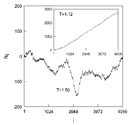
FIG. 1.: Walk profiles obtained from equilibrium spin configurations of the Ising model ($q=2$) at $T=1.50>T_{c}^{(q=2)}$ and $T=1.12<T_{c}^{(q=2)}$ (inset).

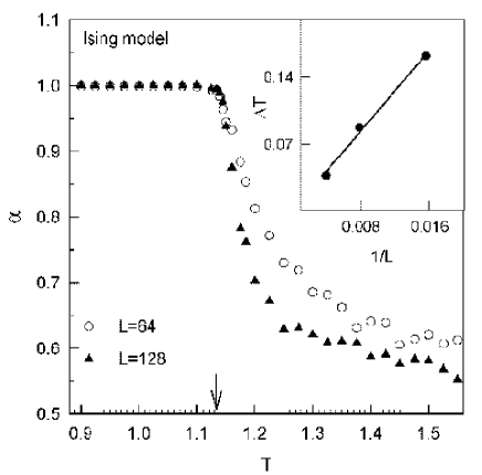
FIG. 2.: The roughness exponent $\alpha$ as a function of temperature for the Ising model with system sizes $L=64$ and $L=128$. The arrow indicates the static critical temperature $T_{c}^{(q=2)}$. The inset shows the behavior of the width $\Delta T$ (see text) with the inverse of the system size $N$, indicating that $\alpha(T)$ is a step function at the $N\rightarrow\infty$ limit.

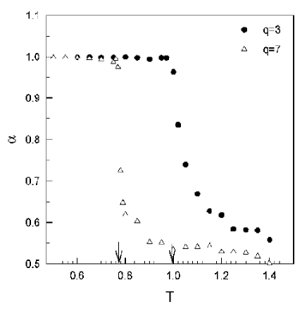
FIG. 3.: The roughness exponent $\alpha$ as a function of temperature for the $q=3$ and $q=7$ Potts model with $L=128$. For $q=3$ the model exhibits a second order phase transition, and for $q=7$ a first order one. The arrows indicate the static critical temperatures $T_{c}^{(q=3)}$ and $T_{c}^{(q=7)}$.

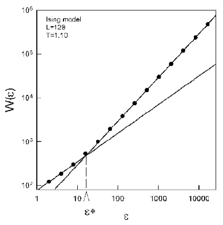
FIG. 4.: A typical log-log plot of $W(\epsilon)\times\epsilon$ used to determine the roughness exponent $\alpha$ characterizing a profile obtained from an Ising spin equilibrium configuration for $T=1.10<T_{c}^{(q=2)}$. We can see clearly a length scale $\epsilon^{*}$ which marks a change in the slope of the fitted straight lines.

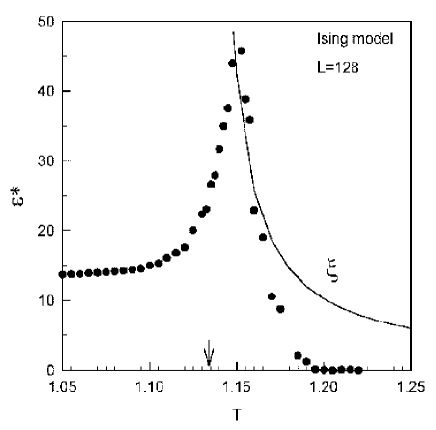
FIG. 5.: The characteristic length $\epsilon^{*}$ as a function of temperature $T$ for the Ising model with system size $L=128$. $\epsilon^{*}$ exhibits a maximum around the critical temperature of the model. The solid curve represents the exact behavior for the correlation length $\xi$ in the disordered phase. The arrow indicates the static critical temperature $T_{c}^{(q=2)}$.

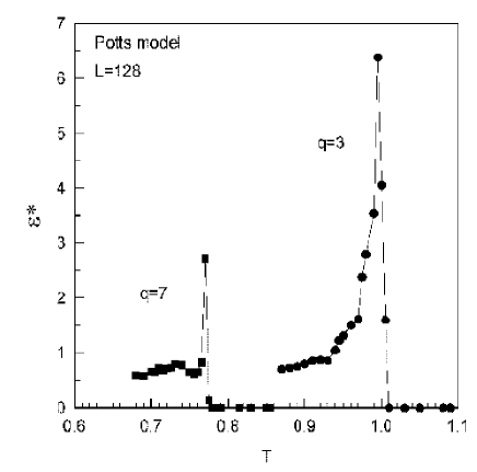
FIG. 6.: The characteristic length $\epsilon^{*}$ as a function of temperature $T$ for the $q=3$ and $q=5$ Potts models with system size $L=128$.

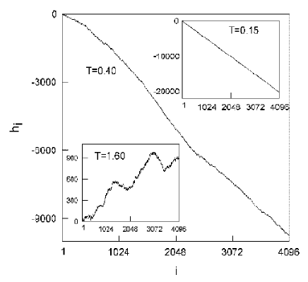
FIG. 7.: Walk profiles obtained from equilibrium spin configurations of the $p=10$ clock model. $T=0.15$ is located in the ordered phase, $T=0.40$ is in the spin-wave phase and $T=1.60$ is in the disordered one.

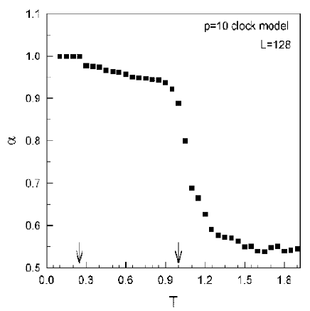
FIG. 8.: The roughness exponent $\alpha$ as a function of temperature for the $p=10$ clock model with system size $L=128$. This model exhibits a Kosterlitz-Thouless type phase transition at $T\simeq 0.24$.

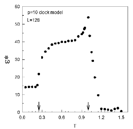
FIG. 9.: The characteristic length $\epsilon^{*}$ as a function of temperature $T$ for the $p=10$ clock model with system size $L=128$. The arrows indicate the static critical temperatures $T_{Ac}^{(p=10)}$ and $T_{Bc}^{(p=10)}$.

REFERENCES

- [1] A. L. Barabási and H. E. Stanley, in Fractal Concepts in Surface Growth (Cambridge University Press, Cambridge, 1995).
- [2] Dynamics of Fractal Surfaces, edited by F. Family and T. Vicsek (World Scientific, Singapore, 1991).
- [3] P. Meakin, in Fractals, Scaling and Growth far from Equilibrium (Cambridge University Press, Cambridge, 1998).
- [4] J. Toner and D. P. DiVincenzo, Phys. Rev. B 41, 632 (1990).
- [5] M. Plischke and B. Bergersen, in Equilibrium Statistical Physics, (World Scientific, Singapore, 1994).
- [6] Spin Glasses and Random Fields, edited by A. P. Young (World Scientific, Singapore, 1998).
- [7] J. A. de Sales, M. L. Martins and J. G. Moreira, Physica A 245, 461 (1997).
- [8] J. A. de Sales, M. L. Martins and J. G. Moreira, J. Phys. A 32, 885 (1999).
- [9] A. P. F. Atman and J. G. Moreira, Eur. Phys. J. B 16, 501 (2000).
- [10] R. M. Ziff, Phys. Rev. Lett. 56, 545 (1986).
- [11] S. Elitzur, R. B. Pearson and J. Shigemitsu, Phys. Rev. D 19, 3698 (1979).
- [12] E. Seiler, I. O. Stamatescu, A. Patrascioiu and V. Linke, Nucl. Phys. B 305 623 (1988).
- [13] B. M. McCoy and T. T. Wu, in The Two-dimensional Ising Model (Harvard Uni. Press, Cambridge, 1973); C. Itzykson and J. M. Drouffe, in Statistical Field Theory vol. I (Cambridge Univ. Press, Cambridge, 1989).
- [14] J. W. Kantelhardt, E. Koscielny-Bunde, Henio H. A. Rego, S. Havlin and A. Bunde, preprint cond-mat/0102214 (2001)