SUNY-NTG-01/02

Spectral properties of a generalized chGUE

A.M. García-García

Department of Physics and Astronomy, SUNY, Stony Brook, New York 11794

Abstract

We consider a generalized chGUE based on a weak confining potential. We study the spectral correlations close to the origin in the thermodynamic limit. We show that for eigenvalues separated up to the mean level spacing the spectral correlations coincide with those of chGUE. Beyond this point, the spectrum is described by an oscillating number variance centered around a constant value. We argue that the origin of such a rigid spectrum is due to the breakdown of the translational invariance of the spectral kernel in the bulk of the spectrum. Finally, we compare our results with the ones obtained from a critical chGUE recently reported in the literature. We conclude that our generalized chGUE does not belong to the same class of universality as the above mentioned model.

PACS: 11.30.Rd, 12.39.Fe, 12.38.Lg, 71.30.+h
Keywords: Chiral ensembles; Spectral Correlations; Critical Statistics

1 Introduction

Critical statistics has been an intense subject of study in recent years [4, 21, 20, 22, 23, 18, 16, 3]. So far, two kinds of models have been proposed to describe those critical correlations. In one of them, deviations from Wigner-Dyson statistics are obtained by adding a symmetry breaking term to the Gaussian Unitary Ensemble (GUE) [20, 10]. The model is solved by mapping it to a non interacting Fermi gas of eigenvalues. The second one [23] makes use of soft confining potentials. It is solved exactly by means of q-orthogonal polynomials.

Universality in critical statistics have been conjectured [21] due to the fact both models share the same kernel in the thermodynamic limit and when the deviations from GUE are small. However, the origin of the critical kernel is different in both cases. In models based in soft confining potentials the critical kernel is obtained from a nontrivial unfolding caused by the strong fluctuations of the spectral density. In models with a explicit breaking symmetry term, deviations from Wigner-Dyson statistics arise because the long range interactions among eigenvalues are suppressed [11]. Although progress have been recently reported [8], the universality class associated with critical statistics can be still considered an unresolved problem.

Recently [10], a critical chiral Gaussian Unitary Ensemble (chGUE) [25] of the first class (addition of a symmetry breaking term to the chGUE) was proposed in order to describe the spectral correlations of the QCD Dirac operator beyond the Thouless energy [5]. It was found that in the bulk of the spectrum and for small deviations from the Wigner-Dyson statistics, the spectral kernel coincided with the one conjectured [21] to be universal for critical statistics. In this letter we shall study the effect of the hard edge (the ensemble is defined on the positive real axis only) on the spectral correlations of a chGUE with a weak confining potential.

We will proceed as follows. First, we propose a random matrix ensemble defined on the positive real line with a non-polynomial potential which is soft confining in the bulk of the spectrum and Gaussian close to the origin. Then, we compute the spectral kernel in the semiclassical approximation. Finally, we compare our model with the above mentioned critical chGUE [10].

Properties of chGUE with weakly confining potentials have already been discussed in the physics literature [28, 4, 14, 6], but attention was focused in the bulk of the spectrum. The effect of the hard edge in the critical spectral correlations and its impact on universality remains an open question.

2 Definition of the Model

In this section we introduce the model to be studied and argue the need to unfold the spectrum. Finally, we compute the mean spectral density needed for such unfolding by using the Dyson’s mean field equation.

We consider a $N\times N$ complex hermitian matrix ensemble $H$ with block structure,

$$H=\left(\begin{array}[]{cr}0&C^{\dagger}\\ C&0\end{array}\right)$$ (3)

and probability distribution given by,

$$P(C)\propto e^{-V(CC^{\dagger})}$$ (4)

where $C$ is a $N/2\times N/2$ hermitian matrix. In terms of the eigenvalues of $H$, the joint distribution is given by,

$$P(x_{1}\ldots x_{N})\propto\prod_{i=1}^{N}x_{i}e^{-V(x_{i})}\prod_{1\leq i<j\leq N}|x_{i}^{2}-x_{j}^{2}|^{2}$$ (5)

$$V(x_{i})=\frac{1}{\gamma}{\rm{arcsinh}}^{2}(x_{i})$$ (6)

where $x_{i}$ are the eigenvalues of $H$.

Since $V(x_{i})$ in (5) is proportional to $x_{i}^{2}$ for $x_{i}\ll 1$ we expect to recover the chGUE kernel [25] in this limit. For $x_{i}\gg 1$, the potential $V(x_{i})\propto\log^{2}(x_{i})$ fail to keep the eigenvalues confined and deviations from the chGUE may be relevant [9].

If the considered interval were the whole real line, the orthogonal polynomials associated with (6) would be the $1/q$- Hermite polynomials $h_{n}(x;q)$ [24, 2, 23] with $\gamma=\log(1/q)$. Unfortunately, for the positive real axes we do not know any set of polynomials orthogonal with respect to the measure (4) with the potential (6). Thus, in order to compute the mean spectral density necessary to unfold the spectrum we shall use the Dyson’s mean field equation.

The joint distribution (5) can be written as a statistical distribution of a one dimensional system of $N$ particles at temperature “$1/T=2$” with a pairwise logarithmic interaction and a one particle potential given by (6) that maintains the system confined.

$$P(x_{1},\ldots x_{N})\propto e^{-F(x_{1},\ldots,x_{N})/T}$$ (7)

where

$$F(x_{1},\ldots,x_{N})=\sum^{N}_{i=1}V(x_{i})-2\sum_{i\neq j}^{N}\log|x_{i}^{2}-x_{j}^{2}|-\log(x_{i})$$ (8)

We want to perform a mean field theory analysis of the above one dimensional system. We assume that in the large $N$ limit the above system has a continuous macroscopic density given by,

$$\rho(\epsilon)=\sum_{i=1}^{N}\delta(\epsilon-\epsilon_{i})$$ (9)

Plugging $\rho(\epsilon)$ into (8) and assuming that the density is non zero only in the interval $0<x<D$ we can express $F$ as a functional of the spectral density.

$$F[\bar{\rho}(\epsilon)]=\int_{0}^{D}\bar{\rho}(\epsilon)V(\epsilon)d\epsilon-\int_{0}^{D}\int_{0}^{D}\bar{\rho}(\epsilon)\bar{\rho}(\epsilon^{\prime})\log|\epsilon-\epsilon^{\prime}|d\epsilon d\epsilon^{\prime}$$ (10)

The mean spectral density $\rho_{MF}$ is defined as the density that minimizes the above functional, namely, $\delta F/\delta\bar{\rho}=0$, that implies

$$\int_{0}^{D}d\epsilon^{\prime}{\rho}(\epsilon_{MF}^{\prime})\log|\epsilon-\epsilon^{\prime}|=V(\epsilon)+c$$ (11)

where $c$ is a constant due to the normalization constraint. The general solution of the above equation (usually called Dyson equation) is given by [12],

$$\rho_{MF}(\epsilon)=\frac{1}{{\pi}^{2}}\sqrt{D^{2}-{\epsilon}^{2}}Re\int_{0}^{D}\frac{dV/dt}{\sqrt{D^{2}-{t}^{2}}}\frac{tdt}{t^{2}-{\epsilon_{+}^{2}}}$$ (12)

where $\epsilon_{+}=\epsilon+i0$. $D$ is found from the normalization condition,

$$\int_{0}^{D}\rho_{MF}(\epsilon)d\epsilon=N$$ (13)

Now, the task is to compute $\rho_{MF}$ for the potential $V(\epsilon)=\frac{1}{\gamma}{\rm{arcsinh}^{2}(\epsilon)}$,

$$\rho_{MF}(\epsilon)=\frac{2}{\gamma{\pi}^{2}}\sqrt{D^{2}-{\epsilon}^{2}}Re\int_{0}^{D}\frac{{\rm{arcsinh}}(t)}{\sqrt{1+t^{2}}}\frac{1}{\sqrt{D^{2}-{t}^{2}}}\frac{tdt}{t^{2}-{\epsilon_{+}^{2}}}$$ (14)

This integral can be performed by changing the contour of integration in a sum of two pieces, $A=A_{1}+A_{2}$ where $A_{1}$ is the the negative imaginary axis and $A_{2}$ is the interval $[D,\infty]$. Since we are interested only in the real part of (14), $A_{2}$ does not contribute to the integral . Thus, (14) can be written as,

$$\rho_{MF}(\epsilon)=\frac{1}{\gamma{\pi}}\sqrt{D^{2}-{\epsilon}^{2}}\frac{2}{\pi}\int_{1}^{\infty}\frac{t}{\sqrt{t^{2}-1}\sqrt{D^{2}+t^{2}}}\frac{1}{t^{2}+{\epsilon}^{2}}$$ (15)

The above integral can be performed by means of a change of variables, the final result being,

$$\rho_{MF}(\epsilon)=\frac{1}{\pi\gamma}\frac{1}{\sqrt{{\epsilon}^{2}+1}}\arctan\frac{\sqrt{D^{2}-{\epsilon}^{2}}}{\sqrt{{\epsilon}^{2}+1}}$$ (16)

From the normalization condition we find that $D=\sinh(\pi\gamma N)$, therefore, the mean spectral density for $N\rightarrow\infty$ is given by,

$$\rho_{MF}(\epsilon)=\frac{1}{2\gamma}\frac{1}{\sqrt{{\epsilon}^{2}+1}}$$ (17)

As expected, $\rho_{MF}(\epsilon)$ has the right limiting values, it is a constant for $\epsilon\ll 1$ (as in the chGUE case) and for $\epsilon\gg 1$ is proportional to $1/\epsilon$, as for the random matrix ensemble with soft confining potentials discussed in [9, 16, 24, 3]. The above spectral density will be used in the next section to unfold the spectrum.

This unfolding allows us to work in units in which the mean level spacing is equal to one. We recall that, in this context, random matrix theories only reproduce spectral correlations around the average spectral density.

We remark that the above mean spectral density is an approximate formula capable of giving only the smooth part of the spectral density. The exact mean spectral density has oscillations which are out of reach of the mean field formalism above used. Therefore, the mean spectral density (17) is only valid approximation if these fluctuation are small enough [16]. In our model this situation corresponds with $\gamma\ll 1$. For $\gamma\gg 1$ the exact spectral density is a rapidly oscillating function. Hence, it is not possible to define a meaningful mean spectral density out of it [16, 9].

As the mean spectral density is not constant, the rescaling procedure is not trivial [11]. The variable $x$ in terms of which the spectral density becomes a constant, is the integrated mean spectral density.

$$x=\int_{0}^{E}\rho_{MF}(\epsilon)d\epsilon$$ (18)

where $\rho_{MF}(\epsilon)$ is the mean spectral density previously found. We shall see in the next section that this nontrivial unfolding is the main ingredient to get a non translational invariant kernel in the bulk of the spectrum.

3 Calculation of the spectral kernel

In this section we compute the spectral kernel in the semiclassical approximation. The semiclassical approximation in the GUE consists in substituting the wave function (orthogonal polynomials times $e^{-V(x)}$) appearing in the spectral kernel, after the Christoffel-Darboux formula is applied, by their WKB approximation. Because of the hard edge at $x=0$ we cannot simply do a WKB approximation by replacing the wave functions by plane waves, but instead have to use Bessel functions.

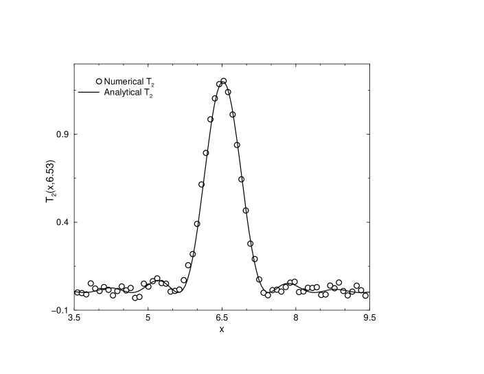
Figure 1: We compare the analytical value of $T_{2}(x,6.53)=|K(x,6.53)|^{2}$ with the numerical one. $K(x,y)$ is given by (23) with $\gamma=0.25$. The numerical integration was performed by using the Metropolis algorithm for $N=100$ “particles” in the confining potential (6). We have used the first $9{\cdot}10^{4}$ sweeps to “warm up” the system and taken the average over the next $9{\cdot}10^{5}$. We repeated the process four times. The final result is the the average of the four trials. We explicitly checked the agreement between numerical and analytical results for $y<20$.

The kernel associated with (6) can be written in terms of the wave function as follows,

$$K(E,E^{\prime})=\frac{\psi_{2N+1}(E)\psi_{2N}(E^{\prime})-\psi_{2N+1}(E^{\prime})\psi_{2N}(E)}{\pi(E-E^{\prime})}+\frac{\psi_{2N+1}(E^{\prime})\psi_{2N}(E)+\psi_{2N+1}(E^{\prime})\psi_{2N}(E)}{\pi(E+E^{\prime})}$$ (19)

where $\psi_{2N}(E)$ and $\psi_{2N+1}(E)$ are the even and odd large $N$ limit of the wave functions associated with the potential (6). In the semiclassical approximation those functions are given by [9],

$$\psi_{2N}(E)=\sqrt{s(E)}J_{0}(\pi s(E))$$ (20)

$$\psi_{2N+1}(E)=\sqrt{s(E)}J_{1}(\pi s(E))$$

where $J_{0}$ and $J_{1}$ are Bessel functions and $s(E)$ is defined by, $\rho_{MF}=ds/dE$, with $\rho_{MF}$ the mean spectral density computed in the last section. It is clear [7] that the above semiclassical expressions for the wave functions are correct for polynomial increasing potential. For soft confining potentials, according to [16, 9] these expressions are valid if the mean-field spectral density used to unfold the spectrum is close to the exact mean spectral density. In our model this happens whether $\gamma\ll 1$. Othe argument supporting (20) comes from the asymptotic form of the orthogonal polynomials associated with a potential asymptotically proportional to $\log^{2}(E)$. This problem have already been discussed in the literature [4]. They found that for $E\gg 1$, $\Psi_{2N}(E)\propto\cos(\log(E)/\gamma)$. This result coincides with (20) in the limit considered. For $E\ll 1$, $s(E)\propto 1/\gamma$ and we recover the chGUE result. As an additional check, we evaluate $T_{2}(x,y)=|K(x,y)|^{2}$ by numerical integration of the the joint distribution (5). Figure 1 shows that the agreement between numerical and analytical results is excellent. We recall that for polynomial-like increasing potentials the mean spectral density is a constant proportional to $N\gg 1$, $s(E)$ is linear for $E\rightarrow 0$ and we recover the kernel of the chGUE [28].

Once we know the form of the kernel we can unfold the spectrum by using (18) and (17) [11, 14].

$$\int_{0}^{E}\frac{2}{\gamma}\frac{1}{\sqrt{1+{\epsilon}^{2}}}d\epsilon=x$$ (21)

$$E=\sinh(x\gamma/2)$$ (22)

where for convenience we have set $\gamma=\gamma/4$. The kernel in terms of the new, unfolded variables is given by,

$$K(x,y)=\frac{\pi\gamma}{8}\sqrt{\cosh(\gamma x/2)\cosh(\gamma y/2)xy}[\frac{J_{0}(\pi x)J_{1}(\pi y)+J_{0}(\pi y)J_{1}(\pi x)}{\sinh((x+y)\gamma/4)\cosh((x-y)\gamma/4)}+$$

$$\frac{J_{1}(\pi x)J_{0}(\pi y)-J_{1}(\pi y)J_{0}(\pi x)}{\sinh((x-y)\gamma/4)\cosh((x+y)\gamma/4)}]$$ (23)

As expected, for $\gamma\rightarrow 0$ we recover the chGUE kernel. This kernel is already in a suitable form for comparison with the one previously found in [10].

$$K(x,y)=\frac{\pi\gamma}{8}\sqrt{xy}[\frac{J_{0}(\pi x)J_{1}(\pi y)+J_{0}(\pi y)J_{1}(\pi x)}{\sinh((x+y)\gamma/4)}+\frac{J_{1}(\pi x)J_{0}(\pi y)-J_{1}(\pi y)J_{0}(\pi x)}{\sinh((x-y)\gamma/4)}]$$ (24)

Figure 2: Number variance for $\gamma=\log(1/q)=0.1$. It is linear for $L\gg 1$ in the critical chGUE of [10]. In our generalized chGUE is almost constant in the bulk of the spectrum.

Even though both kernels reproduce the chGUE kernel for $\gamma\rightarrow 0$ they are essentially different in the bulk of the spectrum. (24) is translational invariant in the bulk of the spectrum, unlike (23), which is not. The origin of such non traslationally invariant kernel is due to the nontrivial unfolding induced by the mean spectral density. This unfolding prevents from vanishing the second term of the right hand of (19) in the bulk of the spectrum.

In the next section, we shall study the effect of the non-translational invariance of the kernel in the spectral correlations involving many levels by computing the number variance.

4 Discussion of results

In this section we shall see, by computing the number variance, that the spectrum of our model is more rigid than the chGUE one and essentially different from the models describing critical statistics.

In order to observe deviations from chGUE prediction we are going to study long-range correlations of eigenvalues by studying the number variance in an interval $[0,s]$.
The number variance is a statistical quantity which gives a quantitative description of the stiffness of the spectrum. The number variance is obtained by integrating the two-point correlation function including the self-correlations

$$\Sigma^{2}(L)=\int_{0}^{L}dx\int_{0}^{L}dy\left[\delta(x-y)\langle\rho(x)\rangle+R_{2}(x,y)\right].$$ (25)

Figure 3: $\gamma=\log(1/q)=0.3$. A constant number variance is observed in the generalized chGUE when $L\gg 1$. That means the spectrum is even more rigid than the chGUE one.

For the Wigner-Dyson statistics the number variance is proportional to $\log(L)$. Such weakly increasing number variance is not surprising as the eigenvalues repulsion produces a highly rigid spectrum. For the Poisson statistics the number variance is equal to $L$ as expected for eigenvalues which are not correlated. Finally, a number variance proportional to $\chi L$ (for $L\gg 1$ and $\chi\ll 1$) is a signature of critical statistics [17, 15, 14, 18, 27, 16]. The slope $\chi$ is directly related [26] to the multifractality of the wave functions of a disordered system at a delocalization-localization transition.

A linear number variance for $L\gg 1$ with a slope $\chi\ll 1$ was found in the generalized chGUE [10]. However, as it can be observed in Figure 2 and 3, the number variance of our model is almost constant for $L\gg 1$. The oscillating behavior around a constant value is partially due to the self-interactions coming from the first term of the number variance.

Apparently, this result is surprising because random matrix ensembles with broken time invariance based on potentials behaving as $\log^{2}(x)$ asymptotically are supposed to have a linear number variance with slope $\chi$ in the bulk of the spectrum, which is a signature of critical statistics [16, 23]. In principle, one may think that the presence of a hard edge at $x=0$ in our model does not affect the spectral properties in the bulk of the spectrum. We argue that this is not the case.

The hard edge, combined with the soft-confining nature of the potential breaks up the translational invariance of the kernel (23) even in the bulk of the spectrum. In the bulk , the cluster function associated with the kernel (23)is given by,

$$Y_{2}(x,y)\propto[\frac{\sin^{2}(\pi(x-y))}{\sinh^{2}((x-y)\gamma/4)}+\frac{\sin^{2}(\pi(x+y))}{\cosh^{2}((x-y)\gamma/4)}+2\frac{\sin(\pi(x+y))}{\cosh((x-y)\gamma/4)}\frac{\sin(\pi(x-y))}{\sinh((x-y)\gamma/4)}]$$ (26)

where we have used the asymptotic expression of the Bessel functions. By performing elementary integrations, we observe that the leading contribution to the number variance for $L\gg 1$ coming from the first term of $Y_{2}$ (translational invariant part) is $\chi L$ where $\chi$ is a function of $\gamma$ only. On the other hand, the leading contribution of the second term of $Y_{2}$ (non-translational invariant part) to the number variance is $-\chi L$. Therefore, both contributions cancel each other and we are left with a oscillating (around a constant value depending on $\gamma$) number variance coming from the third term of the cluster function. We point out that the above cancelation is mainly due to the non-trivial unfolding used.

Roughly speaking, weak increasing potentials fail to keep the eigenvalues confined. As a consequence, the mean spectral density is in general a strongly oscillating function even in the thermodynamic limit. If $\gamma\ll 1$ the deviations from chGUE are small and we can still define a relevant smooth mean spectral density by using the mean field formalism [9]. The unfolding procedure using this mean spectral density breaks the translational invariance of the kernel in the bulk of the spectrum. This breaking of the translational symmetry produces a spectrum highly correlated and essentially different from the one reported in [10].

We would like to mention that a similar result to the one found in this letter has been reported by Canali and Kravtsov [13, 11] . They studied the spectral properties of a generalized GUE based on a weak confining potential with a $\log^{2}(x)$ asymptotic as well. They noticed that in the bulk of the spectrum for $N\rightarrow\infty$ and $\gamma<<1$, the cluster function $Y_{2}(x,y)$ of that ensemble has strong correlations not only when $x\approx y$, but also when $x\approx-y$. The total cluster function is given by the following non translational invariant relation,

$$Y_{2}(x,y)=\frac{\gamma^{2}}{16{\pi}^{2}}\frac{{\sin}^{2}(\pi(x-y))\cosh(x\gamma/2)\cosh(y\gamma/2)}{\cosh^{2}((x+y)\gamma/4)\sinh^{2}((x-y)\gamma/4)}$$ (27)

They showed that, due to this ‘ghost’ peak, the number variance depends on the interval in which it is calculated.

If the interval is not symmetric with respect to the origin ($[0,s]$ for instance), the system does not feel the strong (non-translational invariant) correlations at $x=-y$. Then, the number variance goes asymptotically like $\chi L$ and the model is supposed to describe critical correlations. However, if the interval is symmetric with respect to the origin , the peak at $x=-y$ of the two point function $Y_{2}(x,y)$ has to be taken into account as well. This contribution drives the asymptotic form of the number variance to a constant value [27, 13, 1], in agreement with the results obtained in this letter.

It is straightforward to connect the number variance in the bulk of the spectrum of [27, 13] with the one studied in this letter. The asymptotic form of the number variance in a interval $[0,s]$ associated with the first two terms of (26) corresponds to the number variance in the interval $[-s/2,s/2]$ of the above mentioned critical GUE. By changing variables $u=-x$,$v=y$ in the expression for the number variance of our model we recover the expression obtained by Canali and Kravtsov. The third term of (26) produces the oscillating behavior observed only in our generalized chGUE.

To sum up, due to the non translational invariance of the kernel contributions coming from the points $x\sim-y$ have to be taken into account. These contributions make the linear term in the number variance vanish.

5 Conclusions

In this letter we have studied the effect of a hard edge in the spectral correlations of a chiral random matrix ensemble with a soft confining potential. We showed that beyond the Thouless energy the spectrum is characterized by an oscillating number variance around a constant value. The spectrum is even more correlated than the chGUE one.

The linear term of the number variance characterizing critical statistics vanishes due to the non-translational invariance of the spectral kernel in the bulk of the spectrum. Thus, the generalized chGUE studied in this letter and the ensemble of [10] (in which a linear number variance was found to be proportional to $\chi L$ for $L>>1$) belong to different universality classes [1].

Acknowledgements I thank Daniel Robles, Prof. Denis Dalmazi, Prof. Y.Chen for important suggestions and useful discussions. I thank Prof. J.J.M Verbaarschot for illuminating discussions and for a critical reading of the manuscript. I am indebted to James Osborn for providing me the program to perform the numerical simulation.

This work was supported by the US DOE grant DE-FG-88ER40388

References

- [1] C.M. Canali, M. Wallin and V.E. Kravtsov, Phys. Rev. B. 51, (1995) 2831.
- [2] N.M. Atakishiyev and A. Frank, K. B. Wolf, J. Math. Phys. 35, (1994) 3253.
- [3] M.P. Pato, Phys. Rev. E 61, (2000) R3291.
- [4] Y.Chen, M.E.H. Ismail and K.A. Muttalib, J.Phys. C 5, (1993) 177.
- [5] J.C Osborn and J.J.M. Verbaarschot, Phys. Rev. Lett. 81, (1998) 268.
- [6] Y.Chen, M.E.H. Ismail and K.A. Muttalib, J. Comp. Appl. Math. 54, (1994) 263.
- [7] Y.Chen and N. Lawrence, J. Phys. A 31 (1998) 1141.
- [8] V.E. Kravtsov and A.M. Tsvelik, Phys. Rev. B 68, (2000) 9888.
- [9] E. Bogomolny, O. Bohigas, and M. P. Pato, Phys. Rev. E 55, (1997) 6707.
- [10] A.M. Garcia-Garcia and J.J.M Verbaarschot, Nucl. Phys. B 586, (2000) 668.
- [11] C.M. Canali and V.E. Kravtsov, Phys. Rev. E 51, (2000) R5185
- [12] N.I. Muskhelisvili, “Singular Integral Equations” (Noordhof, Groningen, 1966).
- [13] C. M. Canali, Phys. Rev. B 53, (1996) 3713.
- [14] C. Blecken,Y.Chen and K.A. Muttalib, J. Phys. A 27, (1994) L563.
- [15] D. Braun and G. Montambaux, Phys. Rev. B 52, (1995) 13903.
- [16] S. Nishigaki, Phys. Rev. E 59,(1999) 2853.
- [17] A. Aronov, V. Kravtsov and I. Lerner, Phys. Rev. Lett. 74, 1174 (1995).
- [18] A. Mirlin, Phys. Rep. 326 (2000) 259; M. Janssen, Phys. Rep. 295,(1998) 1.
- [19] K.A. Muttalib, Y. Chen, M.E.H. Ismail and V.N. Nicopoulos, Phys. Rev. Lett. 71,(1993) 471.
- [20] M. Moshe, H. Neuberger and B. Shapiro, Phys. Rev. Lett. 73, (1994) 1497.
- [21] V. Kravtsov and K. Muttalib, Phys. Rev. Lett. 79, 1913 (1997).
- [22] A.D. Mirlin, Y.V. Fyodorov, F.M. Dittes, J. Quezada and T.H. Seligman, Phys. Rev. E 54, (1996) 3221.
- [23] K.A. Muttalib, Y. Chen, M.E.H. Ismail and V.N. Nicopoulos, Phys. Rev. Lett. 71, (1993) 471.
- [24] M.E.H. Ismail and D.R. Masson, Trans. Amer. Math. Soc. 346, 63 (1994).
- [25] E. Shuryak and J.J.M. Verbaarschot, Nucl. Phys. A 560, 306 (1993);J.J.M. Verbaarschot, Phys. Rev. Lett. 72, (1994) 2531; J.J.M. Verbaarschot and I. Zahed, Phys. Rev. Lett. 70, (1993) 3852.
- [26] J. Chalker, I. Lerner and R. Smith, Phys. Rev. Lett. 77, (1996) 554.
- [27] V. Kravtsov, in Proceedings of Correlated Fermions and Transport in Mesoscopic Systems, Moriond Conference, Les Arcs, 1996, cond-mat/9603166.
- [28] J.Osborn and J.J.M. Verbarschoot, Nucl. Phys. B 525 (1998) 738.