Localized Random Lasing Modes and a New Path for Observing Localization

Localization theory and laser theory were both developed in the sixties. The propagation of quantum and classical waves in disordered media has been well understood [1], while the laser physics has been well established [2, 3] at the same time. It was always assumed that disorder was detrimental to lasing action. However, Letokhov [4] theoretically predicted the possibility of lasing in a random system, called “random laser”. But only after the experimental observations by Lawandy et al. [5], the random laser systems have been studied intensively [6, 7, 8, 9, 10, 11, 12, 13, 14, 15, 16, 17, 18, 19]. Since then, many experiments were carried out that showed a drastic spectral narrowing [6] and a narrowing of the coherent backscattering peak [7]. Recently, new experiments [8, 9] showed random laser action with sharp lasing peaks. To fully explain such an unusual behavior of stimulated emission in random systems, many theoretical models were constructed. John and Pang [10] studied the random lasing system by combining the electron number equations of energy levels with the diffusion equation. Berger et al. [11] obtained the spectral and spatial evolution of emission from random lasers by using a Monte Carlo simulation. Very recently, Jiang and Soukoulis [12, 13], by combining a FDTD method with laser theory [2, 3], were able to study the interplay of localization and amplification. They obtained [12, 13] the field pattern and the spectral peaks of localized lasing modes inside the system. They were able to explain [12, 13] the multi-peaks and the non-isotropic properties in the emission spectra, seen experimentally [8, 9]. Finally, the mode repulsion property which gives a saturation of the number of lasing modes in a given random laser system was predicted. This prediction was checked experimentally by Cao et al. [14].

One very interesting question that has not been answered by previous studies is what is the form of the wavefunction in a random laser system. How does the wavefunction in a random system change as one introduces gain? Does the wavefunction retain its shape in the presence of gain? Another very interesting point is if we can predict a priori, which mode will lase first? What will be its emission wavelength? If we understand these issues, we will be able to design random lasers with the desired emission wavelengths. In addition, we will be able to use the random laser as a new tool to study the localization properties of random systems.

In this paper, we explore the evolution of the wavefunction without and with gain, by the time-independent transfer matrix theory [15, 16, 17, 18, 19], as well as by time-dependent theory [12, 13]. The emission spectra can be also obtained. In addition, we can also use the semi-classical theory of lasing [2, 3] to obtain analytical results for the threshold of lasing, as well as which mode will lase first. This depends on the gain profile, as well as the quality factor $Q$ of the modes before gain is introduced.

Our system is essentially a one-dimensional simplification of the real experiments [8, 9]. It consists of many dielectric layers of real dielectric constant $\varepsilon_{2}=2.56\varepsilon_{0}$ ($\varepsilon_{0}$ is the dielectric permeability of free space) of fixed thickness ($b_{0}=100$ nm), sandwiched between two surfaces, with the spacing between the dielectric layer assumed to be a random variable $a_{n}=a_{0}(1+W)$, where $a_{0}=200$ nm and $W$ has a random value in the range of [-0.7, 0.7]. We choose a 30-cell random system, as the first system of our numerical study. In Fig. 1a, we present the results of the logarithm of the transmission coefficient as a function of frequency $f$. These results were obtained by using the transfer matrix techniques introduced in Ref. 15. Notice that we have three typical resonance peaks (denoted $P_{1}$, $P_{2}$ and $P_{3}$) in the frequency range of 600 to 660 THz. As one can see from Fig. 1a, the linewidths of the three modes are different. $P_{3}$ has the smallest linewidth and therefore the largest $Q$, while $P_{1}$ has the largest linewidth and therefore the smallest $Q$. We have also numerically calculated the wavefunctions corresponding to these three peaks and indeed find out that the more localized wavefunction is the one with the larger $Q$. All the results above were obtained for the case without gain.

According to the semiclassical theory of laser physics [2, 3], we generally use a polarization due to gain $P_{gain}=\varepsilon_{0}\chi(\omega)E=\varepsilon_{0}(\chi^{\prime}(\omega)+i\chi^{\prime\prime}(\omega))E$ to introduce amplifying medium effects. Both $\chi^{\prime}(\omega)$ and $\chi^{\prime\prime}(\omega)$ are proportional to the outside pumping rate $P_{r}$ and can be expressed by the parameters of the gain material [20].

To determine which peak will lase first, we can again use the time-independent transfer matrix method (see Eq. (4) of Ref. 15) with a frequency-$independent$ gain, which means the width of the gain profile is very large. It is well understood that time-independent theory [15, 16, 17, 18, 19] for random lasers can be used to obtain the threshold for lasing. At threshold, the transmission coefficient $T$ goes to infinity. In Fig. 1b, we plot the $log_{10}(T)$ versus $\chi^{\prime\prime}$ for the three peaks $P_{1}$, $P_{2}$ and $P_{3}$. In Fig. 1b, the $P_{3}$ which has the largest $Q$ has the smallest threshold for lasing. So, in the frequency-independent gain case, the transfer matrix method gives that the mode with largest $Q$ will lase first. We have also used the transfer-matrix method with a frequency-dependent gain profile, given as a dotted line in Fig. 1a. We choose the central frequency as $f_{a}=\omega_{a}/2\pi=618.56$ THz, which is exactly between the $P_{1}$ and $P_{2}$, and its width to be $\Delta f_{a}=\Delta\omega_{a}/2\pi=15$ THz. In this case, when we increase the pumping rate $P_{r}$, we find the $P_{2}$ will lase first, then $P_{1}$. So two important conditions determine which mode will lase first, the first is the quality factor of the mode and the second is the gain profile. Experimentally, it is quite often that only part of the random medium has been pumped. Then a third factor comes in, i.e. the spatial overlap of the mode function and the gain region.

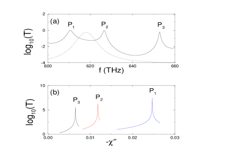
FIG. 1.: (a) Logarithm of transmission coefficient vs frequency of a 30-cell random system with three typical peaks. The dotted line shows the frequency dependent of the gain profile. (b) Logarithm of the transmission coefficient vs $\chi^{\prime\prime}$ for the three peaks shown in Fig. 1a with a frequency-independent gain. $\chi^{\prime\prime}$ is proportional to the pumping rate $P_{r}$.

The next issue we address is the shape of the wave function, as one introduces gain. In Fig. 2a, we present the amplitude of the electric field versus distance for $f=626.6$ THz, which corresponds to the peak $P_{2}$ of Fig. 1a. In Fig. 2b, we show the wavefunction with near-threshold gain at the exact high-peak frequency of $P_{2}$. Both Fig. 2a and 2b are obtained by the time-independent transfer matrix method. Notice that in the presence of gain, the shape of the wavefunction in Fig. 2b is almost same as that without gain in Fig. 2a. The only change is its amplitude which increases uniformly. Actually, by keeping the incident amplitude the same, when we increase the gain from zero to the threshold value, we find that the amplitude of the wavefunction increases from a small to a very large value, but its shape remains almost same.

FIG. 2.: Amplitude of the electric field of the 30-cell system vs $x/x_{0}$, with $x_{0}=5$ nm, for the peak $P_{2}$ in Fig. 1a. (a) Without gain, incident field $E_{inc}=1$V/m; (b) With near-threshold gain ( $P_{r}=7.2\times 10^{6}$/s ), incident field $E_{inc}=1$V/m; (c) The lasing field with over-threshold pumping rate ($P_{r}=2\times 10^{7}$/s . Both (a) and (b) are obtained by the transfer matrix method while (c) is obtained by the FDTD method and laser theory.

To check if indeed this amazing property is also obeyed by the full time-dependent theory [12, 13] of the semiclassical laser theories with Maxwell-equations, we repeat our theory for this case too. While in the time-independent theory, every mode is independent and amplification is not saturated, this is not true for a real lasing system. In a real lasing system, modes will compete with each other. As was discussed in Ref. 12, in a $short$ system, the first lasing mode will suppress all other modes, so we observe only one lasing mode even for a large pumping rate. This is exactly the case when we use the FDTD method to simulate our 30-cell system with an over-threshold gain whose gain profile is the same as given in Fig.1a. At first, the electric field is a random one due to spontaneous emission, then a strong lasing mode evolves from the noisy background and a sharp peak appears in the emission spectrum after Fourier transform. The stable field profile of the FDTD calculation is given in Fig. 2c, where the wavefunction is quite the same as in Fig. 2a and 2b, but the amplitude is very large. The emission spectrum of this case is obtained, and gives a sharp peak very close to the resonant peak $P_{2}$ of Fig. 1a. We also checked the wavefunctions as well as the lasing threshold as we shift the gain profile. If the central frequency of the gain profile is near $P_{3}$, the $P_{3}$ mode will lase first, and the shape of wavefunction of $P_{3}$ remains unchanged. We have also checked the above ideas for a larger ($L\gg\xi$, where $\xi$ is the localization length) system. In such strong localized case, the form of the wavefunction remains unchanged as one introduces gain.

The numerical results which are presented above can be explained by the semi-classical Lamb theory [2] of laser physics. According to Lamb theory, the Maxwell equation of the random laser system can be written as

$$-{\nabla}^{2}{E(x,t)}+\mu_{0}\sigma\frac{\partial E(x,t)}{\partial t}+\mu_{0}\varepsilon(x)\frac{\partial^{2}E(x,t)}{\partial t^{2}}=-\mu_{0}\frac{\partial^{2}P_{gain}(x,t)}{\partial t^{2}}$$ (1)

Where $\mu_{0}$ is the permeability of free space, $E(x,t)$ is the electric field , and the dielectric constant $\varepsilon(x)$ is determined by the random configuration of the system. $\sigma$ is not just the common conductivity loss, but can be interpreted by the total mode loss including the surface loss of the system by radiation. The polarization due to gain $P_{gain}(x,t)$ [20] is the same as the one defined above.

We assume that the system satisfies the slow varying approximation (it is always satisfied if we care about the stable lasing state). So $E(x,t)=E_{m}(t)\phi_{m}(x)exp(-i\omega t)$ (our later discussion shows that the separation of spatial and time parts of wavefunction is reasonable), where $E_{m}(t)$ is the field amplitude, $\phi_{m}(x)$ is the normalized wavefunction, and $\omega$ is the frequency of the field. The surface loss of the mode is $\sigma_{m}=\varepsilon_{0}\omega/Q_{m}$, where the $Q_{m}$ is the quality factor of the mode. Then, we get two equations [2] for the real and the imaginary terms of Eq. (1)

$${\nabla}^{2}{\phi_{m}(x)}+\mu_{0}(\varepsilon(x)+\varepsilon_{0}\chi^{\prime}(x,\omega))\omega^{2}\phi_{m}(x)=0$$ (2)

$$\frac{\partial E_{m}(t)}{\partial t}=\left(-\overline{\chi^{\prime\prime}(\omega)}-\frac{1}{Q_{m}}\right)\frac{\varepsilon_{0}\omega E_{m}(t)}{2\overline{\varepsilon}}$$ (3)

where $\overline{\varepsilon}=\int_{0}^{L}\varepsilon(x)dx/L$ is the spatial averaged dielectric constant inside the system, and $\overline{\chi^{\prime\prime}(\omega)}=\int_{0}^{L}\phi_{m}(x)^{\ast}\chi^{\prime\prime}(x,\omega)\phi_{m}(x)dx/L$ is the spatial averaged gain. The last integral is done to take into account of the overlap between the wavefunction and the spatial region of gain.

Equation (2) determines the field distribution, quality factor $Q_{m}$, and the vibration frequency $\omega$ of the lasing mode. The term $\varepsilon_{0}\chi^{\prime}(x,\omega)$ will cause the vibration frequency to shift away from the original eigenfrequency of the mode, called pulling effect. For a well-defined mode, generally $Q_{m}\gg 1$, we need a very small gain to lase. Then $\chi^{\prime}(x,\omega)\ll 1$, the pulling effect is very weak, and $\omega\simeq\Omega_{m}$, where $\Omega_{m}$ is the eigenfrequency of the mode. So the wavefunction of the lasing mode should be similar to the eigenfunction of the mode. Theoretically, we can use the perturbation method to obtain $\omega$ and the wavefunction.

Equation (3) is the time-dependent amplitude equation. First we can use it to determines the threshold condition when $-\overline{\chi}^{\prime\prime}(\omega)={1}/{Q_{m}}$. For our system, with homogeneous pumping, we have

$$P_{r}^{c}=C_{0}\frac{1+\frac{4(\omega_{a}-\Omega_{m})^{2}}{\Delta\omega_{a}^{2}}}{Q_{m}}$$ (4)

where $C_{0}=\frac{a_{0}+b_{0}}{a_{0}}\frac{\gamma_{c}m_{e}\varepsilon_{0}\omega_{a}\Delta\omega_{a}}{\gamma_{r}N_{0}\tau_{21}e^{2}}$ is a constant. Eq. (4) indeed gives that the threshold value of lasing is inversely proportional to the quality factor $Q$.

Second, Eq. (3) give us the stable amplitude of field when the gain is over threshold. Actually, the gain is saturable, $\chi^{\prime\prime}(\omega)\propto\Delta N\propto 1/(1+C_{2}|E_{m}|^{2})$ [20], in real systems and in our FDTD model [12, 13]. With an over-threshold gain, $E_{m}(t)$ will increase and the gain parameter $\chi^{\prime\prime}(\omega,E_{m})$ will decrease until $-\overline{\chi}^{\prime\prime}(\omega,E_{m})=1/Q_{m}$, then the field is stable. So Eq. (3) also determines the amplitude of the stable field for over-threshold pumping cases.

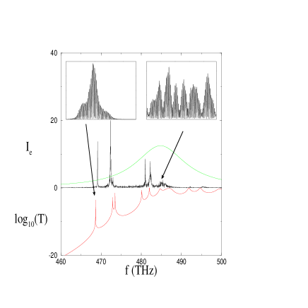
FIG. 3.: Logarithm of the transmission coefficient $T$, the emission intensity $I_{e}$ and the gain profile vs frequency $f$ for a 80-cell random systems. In the insert, wavefunctions of two modes are shown.

Our numerical and analytical results clearly suggest that states of the random system with gain can easily lase, provided their $Q$-factor is large. These findings provide a new path for observing localization of light. Since localized states have large $Q$ values, will lase with a small pumping rate. On the other hand, strongly fluctuating extended states have smaller $Q$ values because of the radiation loss on the surface of the system and can lase only after a stronger pumping. In a real experiment, even in the presence of absorption, if the gain profile is close to the mobility edge, there is going to be a discontinuity in the critical pumping rate needed for lasing. Localized states will lase first at a low pumping rate, while extended states need a high pumping rate. In Fig. 3, we present the results of the DOS vs frequency $f$ for a 1d quasi-disordered system. On the insert two eigenfunctions are given, one localized at $f=468$ THz and the one “extended” at $f=485$ THz. In addition the emission intensity $I_{e}$ vs $f$ is also shown with gain, $P_{r}=10^{5}$ $1/s$, which demonstrate that the localized modes will lase first. In a more realistic 3D case, we expect $I_{e}$ vs frequency to have many peaks for the localized region and no peaks in the extended region for a give pumping rate [21]. It would be very interesting if this discontinuity can be observed experimentally.

In summary, we have used the time-independent transfer matrix method and the FDTD method to show that all lasing modes are coming from the eigenstates of the random system. A knowledge of the eigenstates and the density-of-states of the random system, in conjunction with the frequency profile of the gain, can accurately predict the mode that will lase first, as well as its critical pumping rate. Our detailed numerical results clearly demonstrate that the shape of the wavefunction remains unchanged as gain is introduced into the system. The role of the gain is to just increase uniformly the amplitude of the wavefunction without changing its shape. These results can be understood by generalizing the semi-classical Lamb theory of lasing in random systems. These findings can help us unravel the conditions of observing the localization of light, as well as manufacturing random laser with specific emission wavelengths.

Ames Laboratory is operated for the U.S. Department of Energy by Iowa State University under Contract No. W-7405-Eng-82. This work was supported by the director for Energy Research, Office of Basic Energy Sciences.

REFERENCES

- [1] For a recent review see C. M. Soukoulis and E. N. Economou, Waves Random Media 9, 255 (1999).
- [2] A. Maitland and M. H. Dunn, Laser Physics (North-Holland Publishing Com., Amsterdam, 1969), chapter 9.
- [3] Anthony E. Siegman, Lasers (Mill Valley, California, 1986), chapters 2, 3, 6 and 13.
- [4] V. S. Letokhov, Sov. Phys. JEPT 26, 835 (1968).
- [5] N. M. Lawandy, R. M. Balachandran, S. S. Gomers, and E. Sauvain, Nature 368, 436 (1994).
- [6] W. L. Sha, C. H. Liu and R. R. Alfano, Opt. Lett. 19, 1922 (1994); R. M. Balachandran and N. M. Lawandy, Opt. Lett. 20, 1271 (1995); M. Zhang, N. Cue and K. M. Yoo, Opt. Lett. 20, 961 (1995); G. Van Soest, M. Tomita and A. Lagendijk, Opt. Lett. 24, 306 (1999); G. Zacharakis et. al. Opt. Lett. 25, 923 (2000).
- [7] D. S. Wiersma, M. P. van Albada and Ad Lagendijk, Phys. Rev. Lett. 75, 1739 (1995); D. S. Wiersma and A. Lagendijk, Phys. Rev. E 54, 4256(1996).
- [8] H. Cao et al. Phys. Rev. Lett. 82, 2278 (1999); H. Cao et al. Phys. Rev. Lett. 84 5584 (2000).
- [9] S. V. Frolov, Z. V. Vardeny, K. Yoshino, A. Zakhidov and R. H. Baughman, Phys. Rev. B 59, R5284 (1999).
- [10] S. John and G. Pang, Phys. Rev. A 54, 3642 (1996), and references therein.
- [11] G. A. Berger, M. Kempe, and A. Z. Genack, Phys. Rev. E 56, 6118 (1997).
- [12] Xunya Jiang and C. M. Soukoulis, Phys. Rev. Lett. 85 70 (2000).
- [13] Xunya Jiang and C. M. Soukoulis, in Photonic Crystals and Light Localization in the 21st Century edited by C. M. Soukoulis (Kluwer, Dordrecht, 2001), p. 417.
- [14] H. Cao, Xunya Jiang, C. M .Soukoulis et al. unpublished.
- [15] Xunya Jiang and C. M. Soukoulis, Phys. Rev. B 59, 6159 (1999).
- [16] Xunya Jiang, Qiming Li and C. M. Soukoulis, Phys. Rev. B 59 R9007 (1999).
- [17] P. Pradhan, N. Kumar, Phys. Rev. B 50, 9644 (1994); Z. Q. Zhang, Phys. Rev. B 52, 7960 (1995).
- [18] C. W. J. Beenakker Phys. Rev. Lett. 81, 1829 (1998)
- [19] Qiming Li, K. M. Ho and C. M. Soukoulis, Physica B 296, 78 (2001).
- [20] and , where and , s is the real lifetime of upper lasing level, is the classical decay rate, is number inversion of electrons at upper and lower lasing levels, actually in our FDTD model and real experimental systems so that the gain is saturable for large field amplitude, but when the field is weak ( V/m), the factor is very close to one; and are the central frequency and linewidth of the gain profile; and are the charge and mass of the electron. For a four-level gain medium, , where is the electron density of gain medium, and is the pumping rate. With our parameters, we have . For details see Chap. 2 and 3 and 7 of Ref. 3.
- [21] see Fig. 7c in M. N. Skhunor et. al, Synthetic Metals, 116 485 (2001)