Theory of resonant Raman scattering of tetrahedral amorphous carbon

Abstract

We present a practical method to compute the vibrational resonant Raman spectra in solids with delocalized excitations. We apply this approach to the study of tetrahedrous amorphous carbon. We determine the vibrational eigenmodes and eigenvalues using density functional theory in the local density approximation, and the Raman intensities using a tight binding approximation. The computed spectra are in good agreement with the experimental ones measured with visible and UV lasers. We analyze the Raman spectra in terms of vibrational modes of microscopic units. We show that, at any frequency, the spectra are dominated by the stretching vibrations. We identify a very rapid inversion in the relative Raman intensities of the $sp^{2}$ and $sp^{3}$ carbon sites with the frequency of the incident laser beam. In particular, the spectra are dominated by $sp^{2}$ atoms below 4 eV and by $sp^{3}$ atoms above 6 eV.

I Introduction

Tetrahedral amorphous carbon is a very studied material because of its physical properties, which are close to those of diamond. It is composed of carbon atoms with $sp^{3}$ and $sp^{2}$ hybridization, with a fraction of $sp^{3}$ sites larger than 40 %. The properties of tetrahedral amorphous carbon are very dependent on its microscopic structure. Thus, the knowledge of the microscopic structure can be used to improve the synthesis of the material. Raman spectroscopy have often been applied to the study of tetrahedral amorphous carbon.[1] However visible Raman spectroscopy is much more sensitive to $sp^{2}$ than to $sp^{3}$ carbons.[2] Recently, it has been shown that it is possible to probe the vibrations of $sp^{3}$ carbons with UV Raman,[3, 4] but few UV spectra have been presented in literature up to now. In absence of further experimental data, a theoretical study can elucidate the detailed dependence of the Raman spectra on the laser frequency.

A theory to compute the Raman spectra under non-resonant conditions is well established. Indeed, the Placzek approximation[5] links the scattered Raman intensity with the electronic susceptibility of the sample. However, for resonant Raman the Placzek approximation is not justified. In this work, we develop a practical method for the calculation of resonant Raman spectra in solids with delocalized excitations. We apply this theory to amorphous carbon, using density functional theory in the local density approximation to compute the vibrational modes and frequencies and a tight binding approximation to obtain the resonant Raman intensities. We compare our results to the experimental visible and UV Raman spectra and we analyze our theoretical spectra in terms of the motion of microscopic units.

II Theoretical results

In Raman spectroscopy a sample of matter is irradiated by a monochromatic laser beam of pulsation $\omega_{\rm L}$, and the intensity of the scattered light $I(\omega)$ is measured, as a function of the pulsation $\omega$. The intensity $I(\omega)$ has a main elastic peak at the incident light pulsation, $\omega=\omega_{\rm L}$, and a smaller inelastic contribution at $\omega\neq\omega_{\rm L}$ associated to energy transfers between the light and the sample. In this paper, we will focus on first-order vibrational Stokes spectroscopy, in which the light excites a single vibrational mode.

In order to describe the vibrational Raman scattering and to fix the notation, we need to introduce the Born-Oppenheimer (BO) approximation. Within the BO approximation the eigenstates of the Hamiltonian with eigenvalues $E_{k}^{e}$ can be written as $|\psi_{e,{\bf R}}\rangle\otimes|\nu_{e,k}\rangle$, where the kets $|\psi_{e,{\bf R}}\rangle$ and $|\nu_{e,k}\rangle$ are defined on the Hilbert space of the electronic and nuclear coordinates, respectively. The kets $|\psi_{e,{\bf R}}\rangle$ are the eigenvectors with eigenvalues $E_{e}({\bf R})$ of the electronic Hamiltonian $H^{el}({\bf R})$, which depends parametrically on the positions ${\bf R}$, of the N nuclei (${\bf R}$ represents a vector of 3N coordinates). For every $e$, each $E_{e}({\bf R})$ defines a BO potential energy surface. Finally the wave-functions $|\nu_{e,k}\rangle$ satisfy the eigenvalue equation:

$$[T+E_{e}({\bf R})]|\nu_{e,k}\rangle=E_{k}^{e}|\nu_{e,k}\rangle,$$ (1)

where $T$ is the kinetic energy of the nuclei. It is possible to define a vibrational energy as:

$$\epsilon_{k}^{e}=E_{k}^{e}-E_{e}({\bf R}^{\rm eq}_{e}),$$ (2)

where ${\bf R}^{\rm eq}_{e}$ is the equilibrium position of the nuclei on the BO surface $E_{e}({\bf R})$.

In vibrational Raman spectroscopy, before the scattering, the system is on the ground state BO surface, $E_{0}({\bf R})$, and in the vibrational state $\epsilon_{i}^{0}$, after the scattering the system is still on the ground state BO surface but in a different vibrational state $\epsilon_{f}^{0}$. In first-order Stokes Raman the harmonic approximation is assumed and the final state differs from the initial one by the creation of a phonon with energy $\omega_{s}$.[6]

In non-resonant Raman scattering the energy of incident light is very far from any electronic excitation. Under this condition, a simple and well established theory to compute the scattering intensity $I(\omega)$, have been developed by Placzek.[7, 5] Within the Placzek’s approximation the intensity of scattered light is expressed in terms of the electronic susceptibility at the laser frequency $\chi_{{\bf u}_{\rm L}{\bf u}}(\omega_{\rm L})$:

$$I({\bf u}_{\rm L},{\bf u},\omega)\propto\sum_{s}\frac{\omega^{4}}{\omega_{s}}\left|\frac{\partial\chi_{{\bf u}_{\rm L}{\bf u}}(\omega_{\rm L})}{\partial Q_{s}}\right|^{2}(\langle n_{s}\rangle+1)\delta(\omega-\omega_{\rm L}+\omega_{s}),$$ (3)

where ${\bf u}_{\rm L}$ and ${\bf u}$ are the polarization of the incident and scattered light, $\langle n_{s}\rangle=[\exp(\omega_{s}/(k_{B}T))-1]^{-1}$ is the average thermal occupation of the vibrational state $s$, and the derivative of the susceptibility with respect to the vibrational normal mode $Q_{s}$ is:

$$\frac{\partial\chi_{{\bf u}_{\rm L}{\bf u}}(\omega_{\rm L})}{\partial Q_{s}}=\sum_{J}\sum_{\alpha=x,y,z}\frac{\partial\chi_{{\bf u}_{\rm L}{\bf u}}(\omega_{\rm L})}{\partial R_{J}^{\alpha}}q_{J}^{\alpha,s}=\frac{\partial\chi_{{\bf u}_{\rm L}{\bf u}}(\omega_{\rm L})}{\partial{\bf R}}\cdot{\bf q}^{s}.$$ (4)

Here $q_{J}^{\alpha,s}$ is a component of the unit vector of normal mode $Q_{s}$ for vibration $s$ on the atom J with normalization ${\bf q}^{s}\cdot{\bf q}^{s^{\prime}}=\delta_{s,s^{\prime}}$. The Placzek’s approximation have been used successfully for the first principles computation of the non-resonant vibrational Raman intensity, (see e.g. Refs. [8, 9]).

In resonant Raman spectroscopy the energy of incident light is in resonance with an electronic transition. Under this condition the Placzek’s approximation is, in principle, not justified. However Eq.(3) has also been applied to resonant Raman scattering in solids[10] in order to interpret experimental measurements on semiconductors.

In this paper, we will derive an expression for the scattering intensity in solids which is valid both in the non-resonant and resonant case. This derivation will be used in the following section to analyze the Raman spectra of amorphous carbon.

We start our derivation from the general expression for the vibrational Raman intensity, which can be obtained from theory of second quantization of light:[11]

$$I({\bf u}_{\rm L},{\bf u},\omega) \propto \sum_{i,f}\rho(i)\omega^{4}|{\mathcal{A}}_{i,f}|^{2}\delta(\omega-\omega_{\rm L}-\epsilon_{i}^{0}+\epsilon_{f}^{0}),$$ (5)

with

$${\mathcal{A}}_{i,f}=\sum_{e,k}\left(\frac{\langle\nu_{0,i}|f^{e}_{{\bf u}_{\rm L}}({\bf R})|\nu_{e,k}\rangle\ \langle\nu_{e,k}|f_{{\bf u}}^{e\ast}({\bf R})|\nu_{0,f}\rangle}{E_{e}({\bf R}^{\rm eq}_{e})+\epsilon_{k}^{e}-E_{0}({\bf R}^{\rm eq}_{0})+\epsilon_{i}^{0}-\omega_{\rm L}-i\gamma}\right.$$ (7)

$$\left.+\frac{\langle\nu_{0,i}|f^{e}_{{\bf u}}({\bf R})|\nu_{e,k}\rangle\ \langle\nu_{e,k}|f_{{\bf u}_{\rm L}}^{e\ast}({\bf R})|\nu_{0,f}\rangle}{E_{e}({\bf R}^{\rm eq}_{e})+\epsilon_{k}^{e}-E_{0}({\bf R}^{\rm eq}_{0})+\epsilon_{i}^{0}+\omega+i\gamma}\right).$$

Here, $\rho(i)$ is the probability to find the system in the initial state $i$, $\gamma$ is a small real number added for calculation in order to treat correctly the poles of the expression and

$$f^{e}_{\bf u}({\bf R})=\frac{1}{\sqrt{V}}\langle\psi_{0,{\bf R}}|{\bf u}\cdot{\bf D}({\bf r},{\bf R})|\psi_{e,{\bf R}}\rangle,$$ (8)

where ${\bf D}$ is the ionic and electronic dipole moment, $V$ is the sample volume, and ${\bf r}$ is the position vector for the electrons. Placzek’s expression, Eq. (3), has been derived in the non resonant case starting from Eq. (7).[7, 5] Notice that Eq. (7) is much more complicated to be evaluated than the Placzek’s expression, Eq. (3), since it requires the knowledge of the vibrational eigenfunctions, $|\nu_{e,k}\rangle$, on the excited BO surfaces.

Before presenting our derivation we recall, for comparison, that of the Placzek’s approximation.[7, 5] In the Placzek derivation Eq. (7) is approximated by:

$${\mathcal{A}}_{i,f}=\sum_{e}\left(\frac{\sum_{k}\langle\nu_{0,i}|f^{e}_{{\bf u}_{\rm L}}({\bf R})|\nu_{e,k}\rangle\ \langle\nu_{e,k}|f_{{\bf u}}^{e\ast}({\bf R})|\nu_{0,f}\rangle}{E_{e}({\bf R})-E_{0}({\bf R})-\omega_{\rm L}-i\gamma}\right.$$ (10)

$$\left.+\frac{\sum_{k}\langle\nu_{0,i}|f^{e}_{{\bf u}}({\bf R})|\nu_{e,k}\rangle\ \langle\nu_{e,k}|f_{{\bf u}_{\rm L}}^{e\ast}({\bf R})|\nu_{0,f}\rangle}{E_{e}({\bf R})-E_{0}({\bf R})+\omega+i\gamma}\right).$$

Using the completeness relation $\sum_{k}|\nu_{e,k}\rangle\langle\nu_{e,k}|=1$, Eq. (10) becomes:

$${\mathcal{A}}_{i,f}=\sum_{e}\left(\frac{\langle\nu_{0,i}|f^{e}_{{\bf u}_{\rm L}}({\bf R})f_{{\bf u}}^{e\ast}({\bf R})|\nu_{0,f}\rangle}{E_{e}({\bf R})-E_{0}({\bf R})-\omega_{\rm L}-i\gamma}+\frac{\langle\nu_{0,i}|f^{e}_{{\bf u}}({\bf R})f_{{\bf u}_{\rm L}}^{e\ast}({\bf R})|\nu_{0,f}\rangle}{E_{e}({\bf R})-E_{0}({\bf R})+\omega+i\gamma}\right),$$ (11)

which finally leads to Eq. (3). In order to obtain Eq. (10), we drop the dependence of the denominators of Eq. (7) on the excited vibrational states $|\nu_{e,k}\rangle$, by replacing $[E_{e}({\bf R}^{\rm eq}_{e})+\epsilon_{k}^{e}-E_{0}({\bf R}^{\rm eq}_{0})+\epsilon_{i}^{0}]$ with $[E_{e}({\bf R})-E_{0}({\bf R})]$. In this way, we neglect in the denominators an energy term

$$\Delta_{e}^{k}=E_{e}({\bf R}^{\rm eq}_{e})-E_{e}({\bf R})+\epsilon_{k}^{e}-[E_{0}({\bf R}^{\rm eq}_{0})-E_{0}({\bf R})+\epsilon_{i}^{0}].$$ (12)

This approximation is justified if $E_{e}({\bf R})-E_{0}({\bf R})-\omega_{\rm L}\gg\Delta_{e}^{k}$. Since we are using the completeness relation, the above inequality should, in principle, held for every vibrational states $k$, and not just for the one phonon excitations. In particular, the relation must be verified for excitations, and energy differences $\Delta_{e}^{k}$, involving an arbitrary number of phonons and even for unbounded states in the energy continuum. This condition can obviously never be satisfied. The use of Placzek approximation relies on the hope that the inclusion of excitations involving a limited amount of phonons are sufficient to fulfill the completeness relation. When the laser frequency is close to an electronic transition, the Placzek’s approximation could not be applied in general since, in this case, the dependence on $\Delta_{e}^{k}$ could not be ignored and the completeness relation could not be used.

Here, to compute the Raman spectra in a periodic solid, we simplify Eq. (7) using an approximation different from Placzek’s. In a periodic solid with dispersive bands, the electronic excitations are generally delocalized. In this case, the excited BO surfaces are obtained from the ground-state one by a constant vertical displacement, and we can assume that $|\nu_{e,k}\rangle\simeq|\nu_{0,k}\rangle$, ${\bf R}^{\rm eq}_{e}\simeq{\bf R}^{\rm eq}_{0}$, and $\epsilon_{k}^{e}\simeq\epsilon_{k}^{0}$. This leads to:

$${\mathcal{A}}_{i,f}({\bf u}_{\rm L},{\bf u})=\sum_{e,k}\left(\frac{\langle\nu_{0,i}|f^{e}_{{\bf u}_{\rm L}}({\bf R})|\nu_{0,k}\rangle\ \langle\nu_{0,k}|f_{\bf u}^{e\ast}({\bf R})|\nu_{0,f}\rangle}{E_{e}({\bf R}^{\rm eq}_{0})-E_{0}({\bf R}^{\rm eq}_{0})+\epsilon_{k}^{0}-\epsilon_{i}^{0}-\omega_{\rm L}-i\gamma}\right.$$ (14)

$$\left.+\frac{\langle\nu_{0,i}|f^{e}_{\bf u}({\bf R})|\nu_{0,k}\rangle\ \langle\nu_{0,k}|f_{{\bf u}_{\rm L}}^{e\ast}({\bf R})|\nu_{0,f}\rangle}{E_{e}({\bf R}^{\rm eq}_{0})-E_{0}({\bf R}^{\rm eq}_{0})+\epsilon_{k}^{0}-\epsilon_{i}^{0}+\omega+i\gamma}\right).$$

We expand the expression of $f^{e}_{{\bf u}}({\bf R})$ at first order around ${\bf R}^{\rm eq}_{0}$, $f^{e}_{{\bf u}}({\bf R})\simeq f^{e}_{{\bf u}}({\bf R}^{\rm eq}_{0})+({\bf R}-{\bf R}^{\rm eq}_{0})\cdot\partial f^{e}_{\bf u}({\bf R}^{\rm eq}_{0})/\partial{\bf R}$ and we extract all the terms of degree one in $({\bf R}-{\bf R}^{\rm eq}_{0})$ in Eq. (14). The term ${\bf R}-{\bf R}^{\rm eq}_{0}$ can be written using the operators of creation and annihilation of one phonon of energy $\omega_{s}$. If we extract Stokes terms, we can write the amplitude as a function of a vibration $s$,

$$I({\bf u}_{\rm L},{\bf u},\omega) \propto \sum_{s,n_{s}}\rho(n_{s})\omega^{4}|{\mathcal{A}}_{s}|^{2}\delta(\omega-\omega_{\rm L}+\omega_{s}),$$ (15)

where $n_{s}$ is the occupation number of the mode $s$, $\omega_{s}=\epsilon_{f}^{0}-\epsilon_{i}^{0}$, and

$${\mathcal{A}}_{s} = \sum_{e}\sqrt{\frac{n_{s}+1}{2\omega_{s}}}\left(\frac{{\bf q}_{s}\cdot(\frac{\partial f^{e}_{{\bf u}_{\rm L}}}{\partial{\bf R}})_{{\bf R}^{\rm eq}_{0}}f_{\bf u}^{e\ast}({\bf R}^{\rm eq}_{0})}{E_{e}({\bf R}^{\rm eq}_{0})-E_{0}({\bf R}^{\rm eq}_{0})+\omega_{s}-\omega_{\rm L}-i\gamma}+\frac{f^{e}_{{\bf u}_{\rm L}}({\bf R}^{\rm eq}_{0}){\bf q}_{s}\cdot(\frac{\partial f_{\bf u}^{e\ast}}{\partial{\bf R}})_{{\bf R}^{\rm eq}_{0}}}{E_{e}({\bf R}^{\rm eq}_{0})-E_{0}({\bf R}^{\rm eq}_{0})-\omega_{\rm L}-i\gamma}\right.$$ (16)

$$+ \frac{{\bf q}_{s}\cdot(\frac{\partial f^{e}_{\bf u}}{\partial{\bf R}})_{{\bf R}^{\rm eq}_{0}}f_{{\bf u}_{\rm L}}^{e\ast}({\bf R}^{\rm eq}_{0})}{E_{e}({\bf R}^{\rm eq}_{0})-E_{0}({\bf R}^{\rm eq}_{0})+\omega_{\rm L}+i\gamma}\left.+\frac{f^{e}_{\bf u}({\bf R}^{\rm eq}_{0}){\bf q}_{s}\cdot(\frac{\partial f_{{\bf u}_{\rm L}}^{e\ast}}{\partial{\bf R}})_{{\bf R}^{\rm eq}_{0}}}{E_{e}({\bf R}^{\rm eq}_{0})-E_{0}({\bf R}^{\rm eq}_{0})+\omega_{\rm L}+i\gamma-\omega_{s}}\right).$$ (17)

Finally, we neglect the dependence of the denominator over $\omega_{s}$. Indeed, we expect that ${\mathcal{A}}_{s}$ has the same behavior with respect to $\omega_{L}$ as the electronic susceptibility, $\chi(\omega_{L})$. In a solid with delocalized excitations, away from the van Hove singularities, $\chi(\omega_{L})$ is a smooth function such that $\chi(\omega_{L}\pm\omega_{s})\simeq\chi(\omega_{L})$. Therefore, we expect that in a solid with delocalized excitations we can drop the term $\pm\omega_{s}$ in the denominator of Eq. (16). Notice that the validity requirements of our approximation are less stringent than those of the Placzek’s approximation. Our approximation neglects the dependence of the denominators on the one phonon excitation energies $\omega_{s}$, whereas the Placzek’s approximation neglects the multi-phonons excitation energies $\Delta_{e}^{k}$. Therefore our approximation requires that $\chi(\omega)$ is flat on the energy scale of one phonon excitations whereas the Placzek’s approximation requires that $\chi(\omega)$ is flat on the energy scale of multiple phonon excitations.

$${\mathcal{A}}_{s}=\sqrt{\frac{n_{s}+1}{2\omega_{s}}}\ {\bf q}_{s}\cdot\left.\frac{\partial\kappa({\bf R},{\bf R}^{\prime},\omega_{\rm L})}{\partial{\bf R}}\right|_{{\bf R}={\bf R}^{\prime}={\bf R}^{\rm eq}_{0}},$$ (18)

where

$$\kappa_{{\bf u}_{\rm L},{\bf u}}({\bf R},{\bf R}^{\prime},\omega_{\rm L})=\sum_{e}\frac{f^{e}_{{\bf u}_{\rm L}}({\bf R})f_{\bf u}^{e\ast}({\bf R})}{E_{e}({\bf R}^{\prime})-E_{0}({\bf R}^{\prime})-\omega_{\rm L}-i\gamma}+\frac{f^{e}_{\bf u}({\bf R})f_{{\bf u}_{\rm L}}^{e\ast}({\bf R})}{E_{e}({\bf R}^{\prime})-E_{0}({\bf R}^{\prime})+\omega_{\rm L}+i\gamma}.$$ (19)

Eqs. (15), (18), and (19) are the working expressions that we will use in the next section to compute the Raman intensity.

It is interesting to compare our final expression with that of the Placzek’s approximation. To this purpose we notice that the electronic susceptibility $\chi$ can be obtained as a special case of the function $\kappa$, indeed $\chi_{{\bf u}_{\rm L},{\bf u}}({\bf R},\omega_{\rm L})=\kappa_{{\bf u}_{\rm L},{\bf u}}({\bf R},{\bf R},\omega_{\rm L})$. Thus, the Placzek’s expression differs from the expression we derived just by an additional partial derivative. Indeed, if we assume that

$${\mathcal{A}}_{s}^{\rm Placzek}=\sqrt{\frac{n_{s}+1}{2\omega_{s}}}\ {\bf q}_{s}\cdot\left[\frac{\partial\kappa({\bf R},{\bf R}^{\prime},\omega_{\rm L})}{\partial{\bf R}}+\frac{\partial\kappa({\bf R},{\bf R}^{\prime},\omega_{\rm L})}{\partial{\bf R}^{\prime}}\right]_{{\bf R}={\bf R}^{\prime}={\bf R}^{\rm eq}_{0}},$$ (20)

we obtain Eq. (3) from Eq. (15).

III Calculation on amorphous carbon

We compute the vibrational spectra and the Raman intensities of tetrahedral amorphous carbon using a model generated in Ref. [12] by tight binding (TB) molecular dynamics. The model contains 64 atoms in a periodic cubic cell of 7.57 Å. Among the 64 atoms, 18 atoms are three-fold coordinated ($sp^{2}$ hybridized) and the others are four-fold coordinated ($sp^{3}$ hybridized). In this model all $sp^{2}$ atoms are inserted into a double bonded link, i.e. there are no electronic defects associated to dangling $p$ orbitals. This kind of defects has been identified in other computed generated models of amorphous carbon.[12, 13, 14] Fig. 1 shows a ball and stick model of the $sp^{2}$ carbon atoms in the cell. The $sp^{2}$ atoms are arranged in four pairs and two chains of four and six atoms respectively. No aromatic ring are present in the sample. We compute the dynamical matrix and the vibrational eigenvalues and eigenvectors using density functional theory in the local density approximation.[15] The C atoms are described by a Troullier Martins[16] pseudo-potential with $s$ non-locality. The wave-functions are expanded in a plane wave basis set with a kinetic energy cut-off of 40 Ry. The dynamical matrix is obtained by displacing each atom and computing the resulting forces. The Brillouin zone is sampled with the $\Gamma$ ${\bf k}$-point only. We compute the intensities of the resonant Raman spectra using Eqs. (15), (18), and (19). The evaluation of the intensity at a resonant frequency requires a very fine Brillouin zone k-point mesh, for which a fully ab-initio calculation is not affordable. Therefore we evaluate the function $\kappa_{{\bf u}_{\rm L},{\bf u}}({\bf R},{\bf R}^{\prime},\omega_{\rm L})$ and the electronic susceptibility $\chi_{{\bf u}_{\rm L},{\bf u}}({\bf R},\omega_{\rm L})$ within a TB approximation. We use a TB model with s and p orbitals.[17] We verified that this TB Hamiltonian well reproduces the ab-initio random-phase-approximation (RPA) dielectric constant of diamond[18] for laser frequencies smaller than 10 eV, which is the range of energies used in this work for the calculation of the Raman spectra. The correct description of the dielectric constant for frequencies larger than 10 eV would require the inclusion in the TB model of d or s^∗ orbitals. The Brillouin zone of the 64 atoms supercell is sampled with 108 special k-points. We use a value of 0.05 eV for the constant $\gamma$ in Eq. (19). The derivative in Eq. (18) is computed by numerical differentiation.

In Fig. 2 we present our theoretical vibrational density of state (DOS). The total DOS is decomposed in its partial contributions coming from the $sp^{2}$ and $sp^{3}$ hybridized carbons and from the stretching and bending modes.[19] The $sp^{2}$ vibrations cover the entire range of frequencies of the total DOS, whereas the $sp^{3}$ vibrations form a large peak centered at 1000 $\mbox{cm}^{-1}$, which dies over 1400 $\mbox{cm}^{-1}$. Thus, the modes above 1400 $\mbox{cm}^{-1}$ involve only $sp^{2}$ carbons. The decomposition between bending and stretching contributions shows two separated peaks, centered at 600 $\mbox{cm}^{-1}$ and 1000 $\mbox{cm}^{-1}$, respectively. Above 1000 $\mbox{cm}^{-1}$ the stretching modes contribute alone to the DOS. Similar theoretical results have been presented in Ref. [20] for a model of hydrogenated amorphous carbon.

Before discussing the results for the Raman spectra, we present in Fig. 3 the real and imaginary part of the electronic dielectric constant, $\epsilon(\omega_{L})=1+4\pi\chi(\omega_{L})$. Our theoretical value of 5.8 for the static dielectric constant is in good agreement with the value of 6.2, measured experimentally for a tetrahedral amorphous carbon sample.[21] Notice that, for $\omega>5$ eV, the function $\epsilon(\omega_{L})$ is quite smooth, whereas, under 5 eV, three resonant peaks at 1.3, 3.0 and 3.9 eV show up. The presence of such peaks, which involve transitions between localized $\pi$ states, is an artifact due to the limited size of our model which contains only 9 $\pi$-bonds. This kind of features should disappear in larger models. The electronic structure has a gap of about 0.9 eV, above this value the incident light can be absorbed by the sample, as shown by the non zero value of the imaginary part of the dielectric constant. Thus, Raman spectra both in the visible and ultra-violet (UV) regions are collected under resonant conditions.

Fig. 4 and 5 present the calculated Raman spectra of amorphous carbon for an incident laser beam of 1.8 eV and 4.3 eV, respectively. The laser beam energies are chosen to be away from the three resonant peaks of $\epsilon(\omega_{L})$. For each spectrum, we show a decomposition between $sp^{2}$, $sp^{3}$, bending, and stretching vibrations. We also plot the overlap between the different contributions[22]. The decompositions are meaningful only if the overlap is small. Again, the details of the shape of the Raman spectra coming from $sp^{2}$ atoms are affected by the limited number of $sp^{2}$-$sp^{2}$ bonds in our model. For example the division of the contribution above 1300 $\mbox{cm}^{-1}$ in two peaks is an artifact due to the lack of statistic. In good agreement with the experimental observation,[2] the visible Raman spectrum is essentially due to $sp^{2}$ carbons which give a large contribution above 1200 $\mbox{cm}^{-1}$, centered at 1500 $\mbox{cm}^{-1}$. Only a little $sp^{3}$ contribution, centered at 1000 $\mbox{cm}^{-1}$, can be noticed. In the UV Raman spectrum, on the contrary, a contribution of $sp^{3}$ hybridized atoms can clearly be noticed through the large peak centered at 1000 $\mbox{cm}^{-1}$. Due to a larger number of $sp^{3}$ hybridized atoms in our model, the shape of this peak is more reliable, and its position and shape closely match the experimental results. [3, 4] A peak centered at 1600 $\mbox{cm}^{-1}$, due to $sp^{2}$ sites, can still be observed, as in experiments. Both visible and UV Raman spectra are in a large majority due to the stretching vibrations, only a little contribution of bending vibrations can be noticed at about 600 $\mbox{cm}^{-1}$, which has sometimes been observed in the experimental spectra (see e.g. Fig. 1 of Ref. [3]).

For a given laser pulsation, $\omega_{\rm L}$, we compute the integrated Raman Stokes intensities as the total area of the Stokes spectra. The total integrated Raman intensity and its decomposition in $sp^{2}$, $sp^{3}$, bending, and stretching contributions are presented in Figs. 6 and 7 as a function of $\omega_{\rm L}$. These data show that whatever the energy of the incident light, the intensity of the Raman spectrum is always dominated by stretching modes, whose contribution is always at least an order of magnitude larger than that of bending modes. Regarding the relative decomposition in the $sp^{2}$ and $sp^{3}$ contributions, Fig. 6 and 7 clearly show an inversion at about 5 eV. Under 4 eV almost 90% of the intensity is due to $sp^{2}$ carbons, whereas over 6 eV almost 90% of the intensity is due to $sp^{3}$ carbons. Notice that this inversion happens very quickly, thus, in an experimental measurement a little increase in the energy of the incident light in the UV region can lead to a major modification of the Raman spectra.

Finally, in Fig. 8, we compare the total Raman intensities computed using our method and the Placzek’s approximation. The Raman spectra computed with the Placzek’s approximation show stronger singularities in correspondence to the $sp^{2}-sp^{2}$ electronic transitions. Instead, the intensity of the spectra computed with our approach is similar for laser frequency in resonance with $sp^{2}-sp^{2}$ transitions and with $sp^{3}-sp^{3}$ transitions. We did not find any experimental data for the total intensity as a function of the laser frequency, but according to the discussion of Section II the use of our approximation is more justified in the resonant case.

IV conclusion

In this paper, we have presented a practical method to compute the vibrational resonant Raman spectra in solids. Our approach is justified if the electronic excitations are delocalized. We use our method to compute the vibrational resonant Raman spectra of tetrahedral amorphous carbon. The computed spectra are in good agreement with the experimental ones measured with visible and UV lasers. In particular, the theoretical visible Raman spectra present a broad feature between 1200 and 1700 cm^-1 associated with $sp^{2}$ stretching as found in experiments. In the theoretical UV Raman spectra a second broad peak around 1000 cm^-1 associated to $sp^{3}$ stretching shows up. The location and the shape of this peak agree very well with the experimental UV spectra. We have analyzed in detail the evolution of the Raman spectra as a function of the laser frequency. We have shown that, at any frequency, the spectra are dominated by the stretching vibrations. We have identified a very rapid inversion in the relative Raman intensities of the $sp^{2}$ and $sp^{3}$ sites with the frequency of the incident laser beam. In particular, the spectra are dominated by $sp^{2}$ atoms below 4 eV and by $sp^{3}$ atoms above 6 eV. According to our results, it would be interesting to collect a UV spectrum of tetrahedral amorphous carbon with a laser frequency larger than those used in the actual experiments, to further emphasize the contribution of the tetrahedral $sp^{3}$ carbon sites.

We acknowledge D. A. Drabold for providing us with the model of tetrahedral amorphous carbon. We thank Dr. M. Marangolo for a critical reading of the manuscript. The calculations have been performed at the Idris computer center of the CNRS.

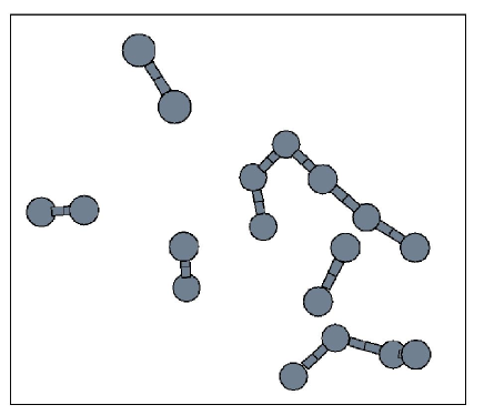
FIG. 1.: A ball and stick model of the $sp^{2}$ carbon atoms in the unit cell. A bond is drawn when the distance between two atoms is less than 1.9 Å. The $sp^{2}$ atoms are arranged in chains, no aromatic ring are present in the model.

FIG. 2.: The total vibrational density of states of tetrahedral amorphous carbon is decomposed in the contributions coming from $sp^{2}$ and $sp^{3}$ carbon sites (upper panel) and in the contributions coming from bending and stretching modes (lower panel). To obtain continuous curves in this figure and in Figs. 4 and 5 we use a Gaussian smearing with $\sigma=50$ $\mbox{cm}^{-1}$.

FIG. 3.: Real and imaginary parts of the electronic dielectric constant of tetrahedral amorphous carbon, $\epsilon(\omega_{\rm L})$, as a function of $\omega_{\rm L}$.

FIG. 4.: Visible Raman spectrum of tetrahedral amorphous carbon computed for $\omega_{\rm L}=1.8$ eV. The Raman intensity is plotted as a function of the Stokes shift, $(\omega_{\rm L}-\omega)$. The total Raman spectrum is decomposed in the contributions coming from $sp^{2}$, $sp^{3}$ atoms, and their overlap (upper panel) and in the contributions coming from stretching and bending vibrations and their overlap (lower panel). Note that the presence of two peaks for energies larger than 1200 cm^-1 is an artifact due to the small total number of $sp^{2}$ sites in our theoretical model.

FIG. 5.: UV Raman spectrum of tetrahedral amorphous carbon computed for $\omega_{\rm L}=4.3$ eV. The Raman intensity is plotted as a function of the Stokes shift, $(\omega_{\rm L}-\omega)$. The total Raman spectrum is decomposed in the contributions coming from $sp^{2}$, $sp^{3}$ atoms, and their overlap (upper panel) and in the contributions coming from stretching and bending vibrations and their overlap (lower panel).

FIG. 6.: Absolute integrated intensities of the Raman spectra of tetrahedral amorphous carbon plotted as a function of the energy of incident laser beam, $\omega_{\rm L}$. In this figure, we present the absolute intensity divided by $\omega^{4}$ (see Eq. (15)) of the 64 atoms model using a logarithmic scale for the intensity axis. The total integrated intensity is decomposed in the contributions coming from $sp^{2}$ and $sp^{3}$ atoms (upper panel) and in the contributions coming from stretching and bending vibrations (lower panel).

FIG. 7.: Fractional integrated intensities of the Raman spectra, plotted as a function of the energy of incident laser beam, $\omega_{\rm L}$. Here, we present the fraction of the $sp^{2}$ and $sp^{3}$ intensity per site. For each value of $\omega_{\rm L}$, we compute the intensities per site, $i^{sp3}(\omega_{\rm L})$ and $i^{sp2}(\omega_{\rm L})$, by dividing the absolute $sp^{3}$ and $sp^{2}$ intensities presented in Fig. 6, by the number of $sp^{3}$ and $sp^{2}$ atoms in the model, respectively. In this figure we plot the fractional intensities, $i^{sp3}(\omega_{\rm L})/[i^{sp3}(\omega_{\rm L})+i^{sp2}(\omega_{\rm L})]$ and $i^{sp2}(\omega_{\rm L})/[i^{sp3}(\omega_{\rm L})+i^{sp2}(\omega_{\rm L})]$.

FIG. 8.: The total integrated intensity of Raman spectra divided by $\omega^{4}$ (see Eq. (15)) computed with Placzek’s approximation and with the approximation developed in this paper, as a function of the incident laser beam energy. We present the intensity in a logarithmic scale.

REFERENCES

• [1] A.ย C. Ferrari and J. Robertson, Phys. Rev. B 61, 14095 (2000), and references therein.
• [2] Q. Wang, D.ย D. Allred, and J. Gonzรกlez-Hernรกndez, Phys. Rev. B 47, 6119 (1993).
• [3] V.ย I. Merkulov etย al., Phys. Rev. Letter 78, 4869 (1997).
• [4] K.ย W.ย R. Gilkes etย al., Appl. Phys. Lett. 70, 1980 (1997).
• [5] P. Brรผesch, Phonons, theory and experiments II : experiments and interpretation of experimental results (Springer-Verlag, Berlin Heidelberg New York, 1986).
• [6] Here and in the following we will use atomic units, with which $\hbar=1$.
• [7] G. Placzek, in Handbuch der Radiologie, edited by E. Marx (Akademische Verlagsgesellschaft, Leipzig, 1934), Vol.ย 6, p.ย 209.
• [8] D. Porezag and M.ย R. Pederson, Phys. Rev. B 54, 7830 (1996).
• [9] P. Giannozzi and S. Baroni, J. Chem. Phys. 100, 8537 (1994).
• [10] P.ย V. Santos etย al., Phys. Rev. B 52, 12158 (1995).
• [11] R. Loudon, The Quantum Theory of Light (Clarendon Press ; Oxford University Press, New York, 1983).
• [12] D.ย A. Drabold, P.ย A. Fedders, and P. Stumm, Phys. Rev. B 49, 16415 (1994).
• [13] F. Mauri, B.ย G. Pfrommer, and S.ย G. Louie, Phys. Rev. Lett. 79, 2340 (1997).
• [14] N. Marks etย al., Phys. Rev. B 54, 9703 (1996).
• [15] J. Hutter etย al., CPMD Version 3.3.5, MPI fรผr Festkรถrperforschung and IBM Research Laboratory, 1990-1998.
• [16] N. Troullier and J.ย L. Martins, Phys. Rev. B 43, 1993 (1991).
• [17] C.ย H. Xu, C.ย Z. Wang, C.ย T. Chan, and K.ย M. Ho, J. Phys. Condens. Matter 4, 6047 (1992).
• [18] L. X. Benedict, E. L. Shirley, and R. B. Bohn, Phys. Rev. B 57, R9385 (1998).
• [19] To perform the projection we have defined for each bond a โ€˜stretchingโ€™ vector in the space of the $3N_{\rm atom}$ displacements. The components of each vector involve the displacement of two atoms in the direction of the bond and with opposite orientations. We use these vectors as a (non-orthonormal) basis of the stretching subspace. We define the bending subspace as the complement of the stretching subspace.
• [20] F. Mauri and A.ย D. Corso, Appl. Phys. Lett. 75, 644 (1999).
• [21] Z.ย Y. Chen and J.ย P. Zhao, J. Appl. Phys. 87, 4268 (2000).
• [22] In the expression of intensity, Eq.ย (15), ๐’œs=๐’œsstretching+๐’œsbendingsubscript๐’œ๐‘ superscriptsubscript๐’œ๐‘ stretchingsuperscriptsubscript๐’œ๐‘ bending{\mathcal{A}}_{s}={\mathcal{A}}_{s}^{\rm stretching}+{\mathcal{A}}_{s}^{\rm bending} where the contributions ๐’œsstretchingsuperscriptsubscript๐’œ๐‘ stretching{\mathcal{A}}_{s}^{\rm stretching} and ๐’œsbendingsuperscriptsubscript๐’œ๐‘ bending{\mathcal{A}}_{s}^{\rm bending} are obtained substituting in Eq.ย (18) the vibrational eigenvector ๐ชssubscript๐ช๐‘ {\bf q}_{s} with its projections in the stretching and bending subspaces, respectively. The intensity is then proportional to |๐’œs|2=|๐’œsstretching|2+|๐’œsbending|2+2โ€‹๐’œsstretchingโ€‹๐’œsbendingsuperscriptsubscript๐’œ๐‘ 2superscriptsuperscriptsubscript๐’œ๐‘ stretching2superscriptsuperscriptsubscript๐’œ๐‘ bending22superscriptsubscript๐’œ๐‘ stretchingsuperscriptsubscript๐’œ๐‘ bending|{\mathcal{A}}_{s}|^{2}=|{\mathcal{A}}_{s}^{\rm stretching}|^{2}+|{\mathcal{A}}_{s}^{\rm bending}|^{2}+2{\mathcal{A}}_{s}^{\rm stretching}{\mathcal{A}}_{s}^{\rm bending}. The first two terms correspond to the contributions of stretching and bending modes, respectively, whereas the last term corresponds to the overlap term. A similar repartition is used to define the sโ€‹p3๐‘ superscript๐‘3sp^{3} and sโ€‹p2๐‘ superscript๐‘2sp^{2} contributions.
Refer to caption
FIG.โ€„1.: A ball and stick model of the sโ€‹p2๐‘ superscript๐‘2sp^{2} carbon atoms in the unit cell. A bond is drawn when the distance between two atoms is less than 1.9 ร…. The sโ€‹p2๐‘ superscript๐‘2sp^{2} atoms are arranged in chains, no aromatic ring are present in the model.
Refer to caption
FIG.โ€„2.: The total vibrational density of states of tetrahedral amorphous carbon is decomposed in the contributions coming from sโ€‹p2๐‘ superscript๐‘2sp^{2} and sโ€‹p3๐‘ superscript๐‘3sp^{3} carbon sites (upper panel) and in the contributions coming from bending and stretching modes (lower panel). To obtain continuous curves in this figure and in Figs. 4 and 5 we use a Gaussian smearing with $\sigma=50$ $\mbox{cm}^{-1}$.
Refer to caption
FIG.โ€„3.: Real and imaginary parts of the electronic dielectric constant of tetrahedral amorphous carbon, $\epsilon(\omega_{\rm L})$, as a function of $\omega_{\rm L}$.
Refer to caption
FIG.โ€„4.: Visible Raman spectrum of tetrahedral amorphous carbon computed for $\omega_{\rm L}=1.8$ eV. The Raman intensity is plotted as a function of the Stokes shift, $(\omega_{\rm L}-\omega)$. The total Raman spectrum is decomposed in the contributions coming from sโ€‹p2๐‘ superscript๐‘2sp^{2}, sโ€‹p3๐‘ superscript๐‘3sp^{3} atoms, and their overlap (upper panel) and in the contributions coming from stretching and bending vibrations and their overlap (lower panel). Note that the presence of two peaks for energies larger than 1200 cm-1 is an artifact due to the small total number of sโ€‹p2๐‘ superscript๐‘2sp^{2} sites in our theoretical model.
Refer to caption
FIG.โ€„5.: UV Raman spectrum of tetrahedral amorphous carbon computed for $\omega_{\rm L}=4.3$ eV. The Raman intensity is plotted as a function of the Stokes shift, $(\omega_{\rm L}-\omega)$. The total Raman spectrum is decomposed in the contributions coming from sโ€‹p2๐‘ superscript๐‘2sp^{2}, sโ€‹p3๐‘ superscript๐‘3sp^{3} atoms, and their overlap (upper panel) and in the contributions coming from stretching and bending vibrations and their overlap (lower panel).
Refer to caption
FIG.โ€„6.: Absolute integrated intensities of the Raman spectra of tetrahedral amorphous carbon plotted as a function of the energy of incident laser beam, $\omega_{\rm L}$. In this figure, we present the absolute intensity divided by $\omega^{4}$ (see Eq.ย (15)) of the 64 atoms model using a logarithmic scale for the intensity axis. The total integrated intensity is decomposed in the contributions coming from sโ€‹p2๐‘ superscript๐‘2sp^{2} and sโ€‹p3๐‘ superscript๐‘3sp^{3} atoms (upper panel) and in the contributions coming from stretching and bending vibrations (lower panel).
Refer to caption
FIG.โ€„7.: Fractional integrated intensities of the Raman spectra, plotted as a function of the energy of incident laser beam, $\omega_{\rm L}$. Here, we present the fraction of the sโ€‹p2๐‘ superscript๐‘2sp^{2} and sโ€‹p3๐‘ superscript๐‘3sp^{3} intensity per site. For each value of $\omega_{\rm L}$, we compute the intensities per site, isโ€‹pโ€‹3โ€‹(ฯ‰L)superscript๐‘–๐‘ ๐‘3subscript๐œ”Li^{sp3}(\omega_{\rm L}) and isโ€‹pโ€‹2โ€‹(ฯ‰L)superscript๐‘–๐‘ ๐‘2subscript๐œ”Li^{sp2}(\omega_{\rm L}), by dividing the absolute sโ€‹p3๐‘ superscript๐‘3sp^{3} and sโ€‹p2๐‘ superscript๐‘2sp^{2} intensities presented in Fig. 6, by the number of sโ€‹p3๐‘ superscript๐‘3sp^{3} and sโ€‹p2๐‘ superscript๐‘2sp^{2} atoms in the model, respectively. In this figure we plot the fractional intensities, isโ€‹pโ€‹3โ€‹(ฯ‰L)/[isโ€‹pโ€‹3โ€‹(ฯ‰L)+isโ€‹pโ€‹2โ€‹(ฯ‰L)]superscript๐‘–๐‘ ๐‘3subscript๐œ”Ldelimited-[]superscript๐‘–๐‘ ๐‘3subscript๐œ”Lsuperscript๐‘–๐‘ ๐‘2subscript๐œ”Li^{sp3}(\omega_{\rm L})/[i^{sp3}(\omega_{\rm L})+i^{sp2}(\omega_{\rm L})] and isโ€‹pโ€‹2โ€‹(ฯ‰L)/[isโ€‹pโ€‹3โ€‹(ฯ‰L)+isโ€‹pโ€‹2โ€‹(ฯ‰L)]superscript๐‘–๐‘ ๐‘2subscript๐œ”Ldelimited-[]superscript๐‘–๐‘ ๐‘3subscript๐œ”Lsuperscript๐‘–๐‘ ๐‘2subscript๐œ”Li^{sp2}(\omega_{\rm L})/[i^{sp3}(\omega_{\rm L})+i^{sp2}(\omega_{\rm L})].
Refer to caption
FIG.โ€„8.: The total integrated intensity of Raman spectra divided by $\omega^{4}$ (see Eq.ย (15)) computed with Placzekโ€™s approximation and with the approximation developed in this paper, as a function of the incident laser beam energy. We present the intensity in a logarithmic scale.