General framework for a portfolio theory with non-Gaussian risks and non-linear correlations

Abstract

Using a family of modified Weibull distributions, encompassing both sub-exponentials and super-exponentials, to parameterize the marginal distributions of asset returns and their natural multivariate generalizations, we give exact formulas for the tails and for the moments and cumulants of the distribution of returns of a portfolio make of arbitrary compositions of these assets. Using combinatorial and hypergeometric functions, we are in particular able to extend previous results to the case where the exponents of the Weibull distributions are different from asset to asset and in the presence of dependence between assets. We treat in details the problem of risk minimization using two different measures of risks (cumulants and value-at-risk) for a portfolio made of two assets and compare the theoretical predictions with direct empirical data. While good agreement is found, the remaining discrepancy between theory and data stems from the deviations from the Weibull parameterization for small returns. Our extended formulas enable us to determine analytically the conditions under which it is possible to “have your cake and eat it too”, i.e., to construct a portfolio with both larger return and smaller “large risks”.

1 Introduction

The determination of the risks and returns associated with a given portfolio constituted of $N$ assets is completely embedded in the knowledge of their multivariate distribution of returns. Indeed, the dependence between random variables is completely described by their joint distribution. This remark entails the two major problems of portfolio theory: 1) determine the multivariate distribution function of asset returns; 2) derive from it useful measures of portfolio risks and use them to analyze and optimize portfolios. Here, we address them both by extending the new approach of [26] in terms of a class of subexponential and superexponential multivariate distributions.

In the standard Gaussian framework, the multivariate distribution takes the form of an exponential of minus a quadratic form $X^{\prime}\Omega^{-1}X$, where $X$ is the unicolumn of asset returns and $\Omega$ is their covariance matrix. The beauty and simplicity of the Gaussian case is that the essentially impossible task of determining a large multidimensional function is collapsed into the very much simpler one of calculating the $N(N+1)/2$ elements of the symmetric covariance matrix. Risk is then uniquely and completely embodied by the variance of the portfolio return, which is easily determined from the covariance matrix. This is the basis of Markovitz’s portfolio theory [17] and of the CAPM (see for instance [18]). In this framework, increasing return comes with risk and return may remunerate a larger risk.

However, the variance (volatility) of portfolio returns provides at best a limited quantification of incurred risks, as the empirical distributions of returns have “fat tails” [16, 8] and the dependences between assets are only imperfectly accounted for by the covariance matrix [15]. Value-at-Risk [11] and other measures of risks [3, 23, 4, 26] have been developed to account for the larger moves allowed by non-Gaussian distributions and nonlinear correlations.

In section 2, we present our parameterization of the multivariate distribution of returns based on two steps: (i) the projection of the empirical marginal distributions onto Gaussian laws via nonlinear mappings; (ii) the use of an entropy maximization to construct the corresponding most parsimonious representation of the multivariate distribution. We show in particular that this construction amounts to use Gaussian copulas. Empirical tests are given which show that this assumption is a very good approxition.

Section 3 offers a specific parameterization of marginal distributions in terms of so-called modified Weibull distributions, which are essentially exponential of minus a power law. This family of distribution contains both sub-exponential and super-exponentials, inclusing the Gaussian law as a special case. Notwithstanding their possible fat-tail nature, all their moments and cumulants are finite and can be calculated. We present empirical calibration of the two key parameters of the modified Weibull distribution, namely the exponent $c$ and the characteristic scale $\chi$.

Section 4 uses the multivariate construction based on (i) the modified Weibull marginal distributions and (ii) the Gaussian copula to derive the asymptotic analytical form of the tail of the distribution of returns of a portfolio composed of an arbitrary combination of these assets. We show that, in the case where individual asset returns have the asymptotic tail $\exp[-(x_{i}/\chi_{i})^{c}]$ with the same exponent $c$, then the tail of the distribution of portfolio return $S$ is of the same form $\exp[-(S/\chi)^{c}]$, with the same exponent $c$ but with a characteristic scale $\chi$ taking different functional forms depending on the value of $c$ and the strength of the dependence between the assets. $\chi$ is also of course a function of the asset weights in the portfolio. These results allow one to estimate the value-at-risk (VaR) in this non-Gaussian nonlinear dependence framework.

Section 5 provides the analytical expressions of the cumulants of the distribution of portfolio returns. Cumulants are of interest because they are natural measures of risks, the higher their order, the more weight being given to large risks. Recall that the second cumulant is nothing but the variance, the normalized third-order (resp. fourth-order) cumulant is the skewness (resp. excess kurtosis). This section provides the most general formulas for any possible positive values of the exponents $c$ of the asset return distributions, generalizing generously previous results [26]. In the case of dependent assets, we give the rather cumbersome explicit formulas only for the case of portfolios of two assets. Similar more cumbersome expressions hold for the general case of $N$ assets. This section also offers empirical tests comparing the direct numerical evaluation of the cumulants of financial time series to the values predicted from our analytical formulas using the exponents $c$ and characteristic scales $\chi$ calibrated previously on the same data. Good consistency is found.

Section 6 uses these two sets of results to offer a first approach to portfolio optimization. We use two approaches, one based on the asymptotic form of the tail of the distribution of portfolio returns, the other based on the expression of the cumulants of the distribution of the portfolio returns. In both cases, we show how to generalize the concept of an efficient frontier, initially introduced in the mean-variance space. We extend it using the different measures of risks captured by the tail of the distribution and by the cumulants. The main novel result is an analytical understanding of the conditions under which it is possible to simultaneously increase the portfolio return and decreases its large risks quantified by large-order cumulants. It thus appears that the multidimensional nature of risks allows one to break the stalemate of no better return without more risks. Section 7 concludes.

Before proceeding with the presentation of our results, we set the notations to derive the basic problem addressed in this paper, namely to study the distribution of the sum of weighted random variables with arbitrary marginal distributions and dependence. Consider a portfolio with $n_{i}$ shares of asset $i$ of price $p_{i}(0)$ at time $t=0$ whose initial wealth is

$$W(0)=\sum_{i=1}^{N}n_{i}p_{i}(0)~{}.$$ (1)

A time $\tau$ later, the wealth has become $W(\tau)=\sum_{i=1}^{N}n_{i}p_{i}(\tau)$ and the wealth variation is

$$\delta_{\tau}W\equiv W(\tau)-W(0)=\sum_{i=1}^{N}n_{i}p_{i}(0){{p_{i}(\tau)-p_{i}(0)}\over p_{i}(0)}=W(0)~{}\sum_{i=1}^{N}w_{i}r_{i}(t,\tau),$$ (2)

where

$$w_{i}={n_{i}p_{i}(0)\over\sum_{j=1}^{N}n_{j}p_{j}(0)}~{}$$ (3)

is the fraction in capital invested in the $i$th asset at time $0$ and the return $r_{i}(t,\tau)$ between time $t-\tau$ and $t$ of asset $i$ is defined as:

$$r_{i}(t,\tau)={p_{i}(t)-p_{i}(t-\tau)\over p_{i}(t-\tau)}~{}.$$ (4)

Using the definition (4), this justifies us to write the return $S_{\tau}$ of the portfolio over a time interval $\tau$ as the weighted sum of the returns $r_{i}(\tau)$ of the assets $i=1,...,N$ over the time interval $\tau$

$$S{\tau}={\delta_{\tau}W\over W(0)}=\sum_{i=1}^{N}w_{i}~{}r_{i}(\tau)~{}.$$ (5)

In the sequel, we shall thus consider asset returns as the fundamental variables (denoted $x_{i}$ or $X_{i}$ in the sequel) and study their aggregation properties, namely how the distribution of portfolio return equal to their weighted sum derives for their multivariable distribution. We shall consider a single time scale $\tau$ which can be chosen arbitrarily, say equal to one day. We shall thus drop the dependence on $\tau$, understanding implicitely that all our results hold for returns estimated over time step $\tau$.

2 Estimation of the joint probability distribution of returns of several assets

2.1 A brief exposition and justification of the method

We will use the method of determination of multivariate distributions introduced by Karlen [12] and Sornette et al. [26]. This method consists in two steps: (i) transform each return $x$ into a Gaussian variable $y$ by a nonlinear monotonous increasing mapping; (ii) use the principle of entropy maximization to construct the corresponding multivariate distribution of the transformed variables $y$.

The first concern to address before going any further is whether the nonlinear transformation, which is in principle different for each asset return, conserves the structure of the dependence. In what sense is the dependence between the transformed variables $y$ the same as the dependence between the asset returns $x$? It turns out that the notion of “copulas” provides a general and rigorous answer which justifies our procedure [26].

For completeness, we briefly recall the definition of a copula (for further details about the concept of copula see [20]). A function $C$ : $[0,1]^{n}\longrightarrow[0,1]$ is a $n$-copula if it enjoys the following properties :

• $\forall u\in[0,1]$, $C(1,\cdots,1,u,1\cdots,1)=u$ ,

• $\forall u_{i}\in[0,1]$, $C(u_{1},\cdots,u_{n})=0$ if at least one of the $u_{i}$ equals zero ,

• $C$ is grounded and $n$-increasing i.e the $C$-volume of every boxes whose vertices lie in $[0,1]^{n}$ is positive.

Skar’s Theorem then states that, given an $n$-dimensional distribution function $F$ with continuous marginal distributions $F_{1},\cdots,F_{n}$, there exists a unique $n$-copula $C$ : $[0,1]^{n}\longrightarrow[0,1]$ such that :

$$F(x_{1},\cdots,x_{n})=C(F_{1}(x_{1}),\cdots,F_{n}(x_{n}))~{}.$$ (6)

This elegant result shows that the study of the dependence of random variables can be performed independently of the behavior of the marginal distributions. Moreover, the following result shows that copulas are intrinsic measures of dependence. Consider $n$ continous random variables $X_{1},\cdots,X_{n}$ with copula $C$. Then, if $g_{1}(X_{1}),\cdots,g_{n}(X_{n})$ are strictly increasing on the ranges of $X_{1},\cdots,X_{n}$, the random variables $Y_{1}=g_{1}(X_{1}),\cdots,Y_{n}=g_{n}(X_{n})$ have exactly the same copula $C$ [14]. The copula is thus invariant under strictly increasing tranformation of the variables. This provides a powerful way of studying scale-invariant measures of associations. It is also a natural starting point for construction of multivariate distributions and provides the theorical justification of the method of determination of mutivariate distributions that we will use in the sequel.

2.2 Transformation of an arbitrary random variable into a Gaussian variable

Let us consider the return $X$, taken as a random variable characterized by the probability density $p(x)$. The transformation $y(x)$ which obtains a standard normal variable $y$ from $x$ is determined by the conservation of probability:

$$p(x)dx=\frac{1}{\sqrt{2\pi}}e^{-\frac{y^{2}}{2}}dy\;.$$ (7)

Integrating this equation from $-\infty$ and $x$, we obtain:

$$F(x)=\frac{1}{2}\left[1+\mbox{erf}\left(\frac{y}{\sqrt{2}}\right)\right]\;,$$ (8)

where $F(x)$ is the cumulative distribution of $X$:

$$F(x)=\int_{-\infty}^{x}dx^{\prime}p(x^{\prime})\;.$$ (9)

This leads to the following transformation $y(x)$:

$$y=\sqrt{2}\;\mbox{erf}^{-1}(2F(x)-1)~{},$$ (10)

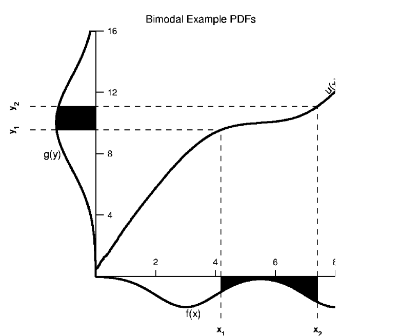
Figure 1: Schematic representation of the nonlinear mapping $Y=u(X)$ that allows one to transform a variable $X$ with an arbitrary distribution into a variable $Y$ with a Gaussian distribution. The probability densities for $X$ and $Y$ are plotted outside their respective axes. Consistent with the conservation of probability, the shaded regions have equal area. This conservation of probability determines the nonlinear mapping.

which is obvously an increasing function of $X$ as required for the application of the invariance property of the copula stated in the previous section. An illustration of the nonlinear transformation (10) is shown in figure 1. Note that it does not require any special hypothesis on the probability density $X$, apart from being non-degenerate.

In the case where the pdf of $X$ has only one maximum, we may use a simpler expression equivalent to (10). Such a pdf can be written under the so-called Von Mises parametrization [5] :

$$p(x)=C\frac{f^{\prime}(x)}{\sqrt{|f(x)|}}e^{-\frac{1}{2}f(x)}\;,$$ (11)

where $C$ is a constant of normalization. For $f(x)/x^{2}\rightarrow 0$ when $|x|\rightarrow+\infty$, the pdf has a “fat tail,” i.e., it decays slower than a Gaussian at large $|x|$.

Let us now define the change of variable

$$y=sgn(x)\sqrt{|f(x)|}\;.$$ (12)

Using the relationship $p(y)=p(x)\frac{dx}{dy}$, we get:

$$p(y)=\frac{1}{\sqrt{2\pi}}e^{-\frac{y^{2}}{2}}\;.$$ (13)

It is important to stress the presence of the sign function $sgn(x)$ in equation (12), which is essential in order to correctly quantify dependences between random variables. This transformation (12) is equivalent to (10) but of a simpler implementation and will be used in the sequel.

2.3 Determination of the joint distribution : maximum entropy and Gaussian copula

Let us now consider $N$ random variables $X_{i}$ with marginal distributions $p_{i}(x_{i})$. Using the transformation (10), we define $N$ standard normal variables $Y_{i}$. If these variables were independent, their joint distribution would simply be the product of the marginal distributions. In many situations, the variables are not independent and it is necessary to study their dependence.

The simplest approach is to construct their covariance matrix. Applied to the variables $Y_{i}$, we are certain that the covariance matrix exists and is well-defined since their marginal distributions are Gaussian. In contrast, this is not ensured for the variables $X_{i}$. Indeed, in many situations in nature, in economy, finance and in social sciences, pdf’s are found to have power law tails $\sim\frac{A}{x^{1+\mu}}$ for large $|x|$. If $\mu\leq 2$, the variance and the covariances can not be defined. If $2<\mu\leq 4$, the variance and the covariances exit in principle but their sample estimators converge poorly.

We thus define the covariance matrix:

$$V=E[{\bf y}{\bf y^{t}}]\;,$$ (14)

where ${\bf y}$ is the vector of variables $Y_{i}$ and the operator $E[\cdot]$ represents the mathematical expectation. A classical result of information theory [22] tells us that, given the covariance matrix $V$, the best joint distribution (in the sense of entropy maximization) of the $N$ variables $Y_{i}$ is the multivariate Gaussian:

$$P({\bf y})=\frac{1}{(2\pi)^{N/2}\sqrt{\det(V)}}\exp\left(-\frac{1}{2}{\bf y^{t}}V^{-1}{\bf y}\right)\;.$$ (15)

Indeed, this distribution implies the minimum additional information or assumption, given the covariance matrix.

Using the joint distribution of the variables $Y_{i}$, we obtain the joint distribution of the variables $X_{i}$:

$$P({\bf x})=P({\bf y})\left|\frac{\partial y_{i}}{\partial x_{j}}\right|\;.$$ (16)

Since

$$\frac{\partial y_{i}}{\partial x_{j}}=\sqrt{2\pi}p_{j}(x_{j})e^{\frac{1}{2}y_{i}^{2}}\delta_{ij}\;,$$ (17)

we get

$$\left|\frac{\partial y_{i}}{\partial x_{j}}\right|=(2\pi)^{N/2}\prod_{i=1}^{N}p_{i}(x_{i})e^{\frac{1}{2}y_{i}^{2}}\;.$$ (18)

This finally yields

$$P({\bf x})=\frac{1}{\sqrt{\det(V)}}\exp\left(-\frac{1}{2}{\bf y_{(x)}^{t}}(V^{-1}-I){\bf y_{(x)}}\ \right)\prod_{i=1}^{N}p_{i}(x_{i})\;.$$ (19)

As expected, if the variables are independent, $V=I$, and $P({\bf x})$ becomes the product of the marginal distributions of the variables $X_{i}$.

Let $F({\bf x})$ denote the cumulative distribution function of x and $F_{i}(x_{i})$ their marginal distributions. The copula $C$ is then such that

$$F(x_{1},\cdots,x_{n})=C(F_{1}(x_{1}),\cdots,F_{n}(x_{n}))~{}.$$ (20)

Differentiating with respect to $x_{1},\cdots,x_{N}$ leads to

$$P(x_{1},\cdots,x_{n})=\frac{\partial F(x_{1},\cdots,x_{n})}{\partial x_{1}\cdots\partial x_{n}}=c(F_{1}(x_{1}),\cdots,F_{n}(x_{n}))\prod_{i=1}^{N}p_{i}(x_{i})~{},$$ (21)

where

$$c(u_{1},\cdots,u_{N})=\frac{\partial C(u_{1},\cdots,u_{N})}{\partial u_{1}\cdots\partial u_{N}}$$ (22)

is the density of the copula $C$.

Comparing (22) with (19), the density of the copula is given in the present case by

$$c(u_{1},\cdots,u_{N})=\frac{1}{\sqrt{\det(V)}}\exp\left(-\frac{1}{2}{\bf y_{(u)}^{t}}(V^{-1}-I){\bf y_{(u)}}\ \right)~{},$$ (23)

which is the “Gaussian copula” with covariance matrix ${\bf V}$. This result clarifies and justifies the method of [26] by showing that it essentially amounts to assume arbitrary marginal distributions with Gaussian copulas. Note that the Gaussian copula results directly from the choice of maximizing the Shannon entropy. This is not unexpected in analogy with the standard result that the Gaussian law is minimizing the Shannon entropy at fixed given variance. If we were to extend this formulation by considering more general expressions of the entropy, such that Tsallis entropy [27], we would have found other copulas.

2.4 Empirical test of the Gaussian copula assumption

We now present preliminary tests of the hypothesis of Gaussian copulas between returns of financial assets. Testing the gaussian copula hypothesis is a delicate task. A priori, two standard methods can be proposed.

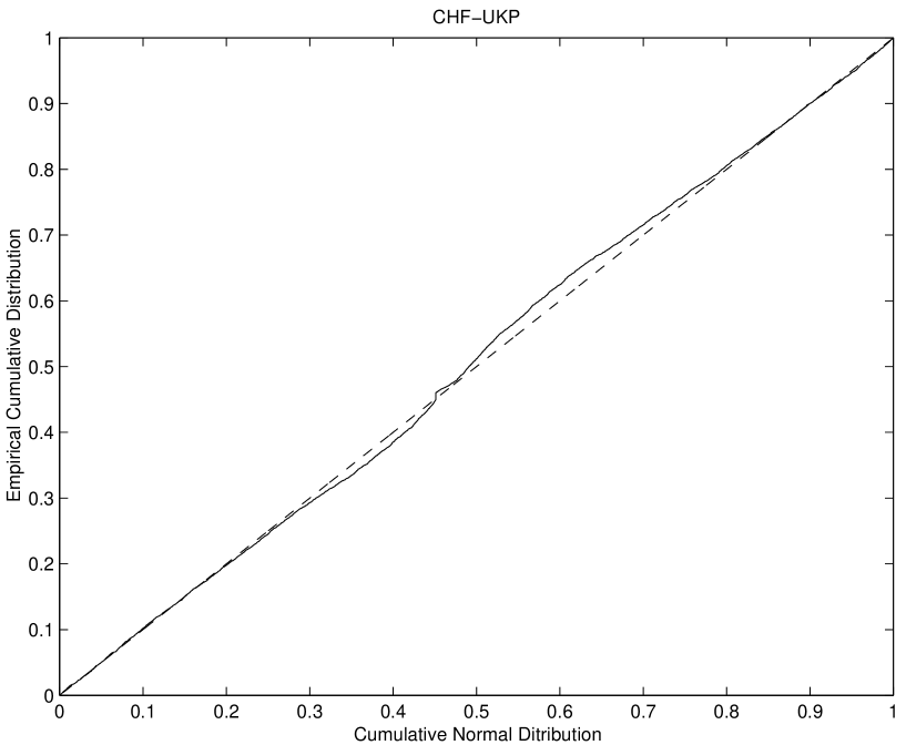
Figure 2: Quantile of the normalized sum of the Gaussianized returns of the Swiss Franc and The British Pound versus the quantile of the Normal distribution, for the time interval from Jan. 1971 to Oct. 1998. Different weights in the sum give similar results.

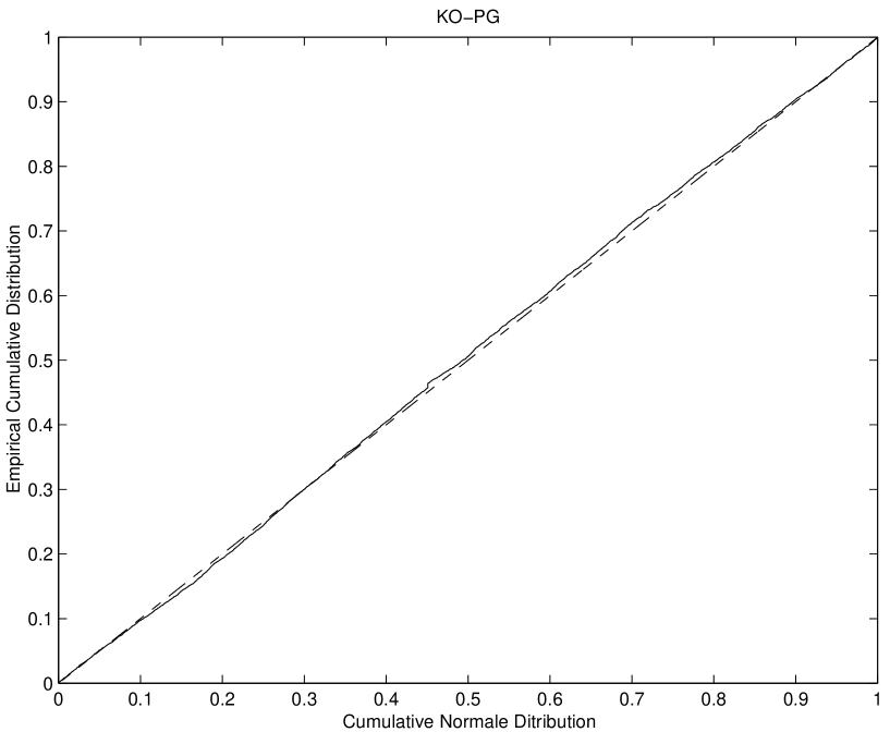
Figure 3: Quantile of the normalized sum of the Gaussianized returns of Coca-Cola and Procter&Gamble versus the quantile of the Normal distribution, for the time interval from Jan. 1970 to Dec. 2000. Different weights in the sum give similar results.

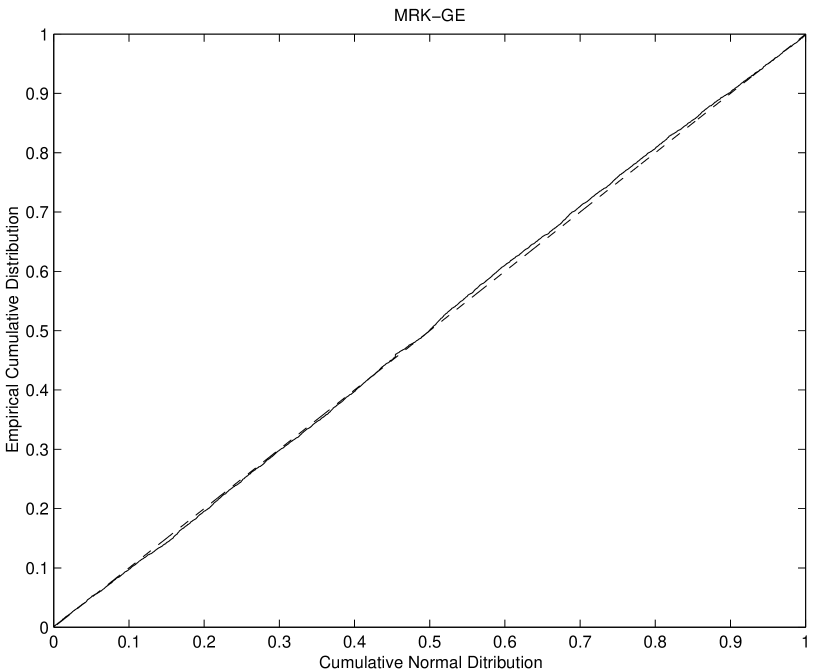
Figure 4: Quantile of the normalized sum of the Gaussianized returns of Merk and General Electric versus the quantile of the Normal distribution, for the time interval from Jan. 1970 to Dec. 2000. Different weights in the sum give similar results.

The first one consists in using that Gaussian variables are stable in distribution under addition. Thus, a (quantile-quantile or $Q-Q$) plot of the cumulative distribution of the sum $y_{1}+\cdots+y_{p}$ versus the cumulative Normal distribution with the same estimated variance should give a straight line in order to qualify a multivariate Gaussian distribution (for the transformed $y$ variables). Such tests on empirical data are presented in figures 2-4.

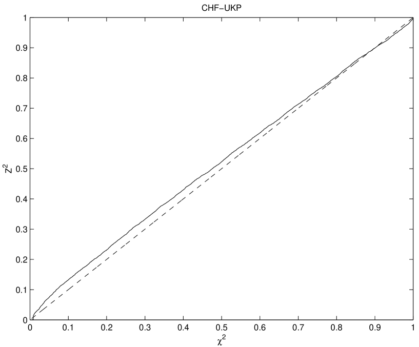
Figure 5: Cumulative distribution of $z^{2}={\bf y^{t}V^{-1}y}$ versus the cumulative distribution of chi-square (denoted $\chi^{2}$) with two degrees of freedom for the couple Swiss Franc / British Pound, for the time interval from Jan. 1971 to Oct. 1998. This $\chi^{2}$ should not be confused with the characteristic scale used in the definition of the modified Weibull distributions.

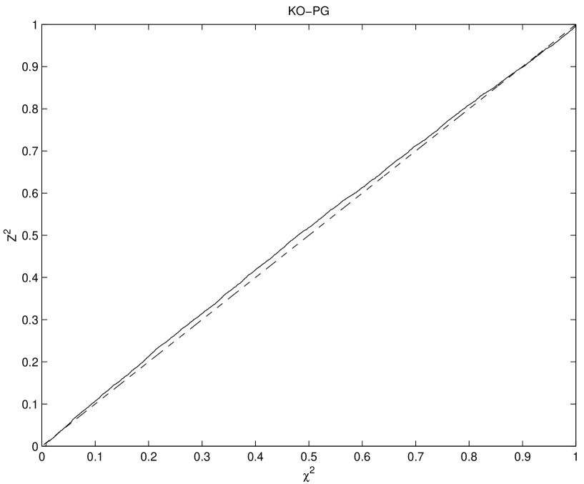
Figure 6: Cumulative distribution of $z^{2}={\bf y^{t}V^{-1}y}$ versus versus the cumulative distribution of the chi-square $\chi^{2}$ with two degrees of freedom for the couple Coca-Cola / Procter&Gamble, for the time interval from Jan. 1970 to Dec. 2000. This $\chi^{2}$ should not be confused with the characteristic scale used in the definition of the modified Weibull distributions.

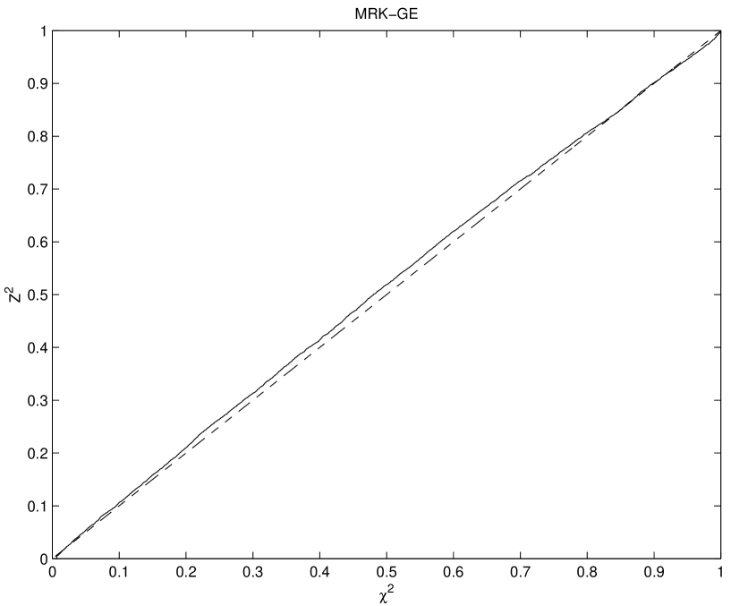
Figure 7: Cumulative distribution of $z^{2}={\bf y^{t}V^{-1}y}$ versus versus the cumulative distribution of the chi-square $\chi^{2}$ with two degrees of freedom for the couple Merk / General Electric, for the time interval from Jan. 1970 to Dec. 2000. This $\chi^{2}$ should not be confused with the characteristic scale used in the definition of the modified Weibull distributions.

The second test amounts to estimating the covariance matrix ${\bf V}$ of the sample we consider. This step is simple since, for fast decaying pdf’s, robust estimators of the covariance matrix are available. We can then estimate the distribution of the variable $z^{2}={\bf y^{t}V^{-1}y}$. It is well known that $z^{2}$ follows a $\chi^{2}$ distribution if ${\bf y}$ is a Gaussian random vector. Again, the empirical cumulative distribution of $z^{2}$ versus the cumulative distribution of $\chi^{2}$ should give a straight line in order to qualify a multivariate Gaussian distribution (for the transformed $y$ variables). Such tests on empirical data are presented in figures 5-7.

First, one can observe that the Gaussian copula hypothesis appears better for stocks than for currencies. Note also that the test of aggregation seems systematically more in favor of the Gaussian copula hypothesis than is the $\chi^{2}$ test, maybe due to its smaller sensitivity. Nonetheless, the very good performance of the Gaussian hypothesis under the aggregation test bears good news for a porfolio theory based on it, since by definition a portfolio corresponds to asset aggregation. Even if sums of the transformed returns are not equivalent to sums of returns (as we shall see in the sequel), such sums qualify the collective behavior whose properties are controlled by the copula.

Notwithstanding some deviations from linearity in figures 2-7, it appears that, for our purpose of developing a generalized portfolio theory, the Gaussian copula hypothesis is a good approximation. A more systematic test of this goodness of fit requires the quantification of a confidence level, for instance using the Kolmogorov test, that would allow us to accept or reject the Gaussian copula hypothesis. However, we have encountered a practical problem to implement this test, as the same sample is used both for the empirical calibration of the covariance and for the test itself. A bootstrap method is thus necessary in order to obtain a real measure of the departure from Gaussianity and thus to decide wether or not these deviations are significant.

3 Choice of an exponential family to parameterize the marginal distributions

3.1 The modified Weibull distributions

We now apply these constructions to a class of distributions with fat tails, that have been found to provide a convenient and flexible parameterization of many phenomena found in nature and in the social sciences [13]. These so-called stretched exponential distributions can be seen to be general forms of the extreme tails of product of random variables [7].

Following [26], we postulate the following marginal probability distributions of returns:

$$p(x)=\frac{1}{2\sqrt{\pi}}\frac{c}{\chi^{\frac{c}{2}}}|x|^{\frac{c}{2}-1}e^{-\left(\frac{|x|}{\chi}\right)^{c}}\;,$$ (24)

where $c$ and $\chi$ are the two key parameters. A more general parameterization taking into account a possible asymmetry between negative and positive returns (thus leading to possible non-zero average return) is

$$p(x) = \frac{1}{2\sqrt{\pi}}\frac{c_{+}}{\chi_{+}^{\frac{c_{+}}{2}}}|x|^{\frac{c_{+}}{2}-1}e^{-\left(\frac{|x|}{\chi_{+}}\right)^{c_{+}}}~{}~{}~{}~{}\mbox{if}~{}x\geq 0$$ (25)

$$p(x) = \frac{1}{2\sqrt{\pi}}\frac{c_{-}}{\chi_{-}^{\frac{c_{-}}{2}}}|x|^{\frac{c_{-}}{2}-1}e^{-\left(\frac{|x|}{\chi_{-}}\right)^{c_{-}}}~{}~{}~{}~{}\mbox{if}~{}x<0~{}.$$ (26)

Thes expressions are close to the Weibull distribution, with the addition of a power law prefactor to the exponential such that the Gaussian law is retrieved for $c=2$. Following [26, 25, 2], we call (24) the modified Weibull distribution. For $c<1$, the pdf is a stretched exponential, also called sub-exponential. The exponent $c$ determines the shape of the distribution, fatter than an exponential if $c<1$. The parameter $\chi$ controls the scale or characteristic width of the distribution. It plays a role analogous to the standard deviation of the Gaussian law. See chapter 6 of [24] for a recent review on maximum likelihood and other estimators of such generalized Weibull distributions.

3.2 Transformation of the modified Weibull pdf into a Gaussian Law

One advantage of the class of distributions (24) is that the transformation into a Gaussian is particularly simple. Indeed, the expression (24) is of the form (11) with

$$f(x)=2\left(\frac{|x|}{\chi}\right)^{c}~{}.$$ (27)

Applying the change of variable (12) which reads

$$y_{i}=sgn(x_{i})~{}\sqrt{2}~{}\left(\frac{|x_{i}|}{\chi_{i}}\right)^{\frac{c_{i}}{2}}\;,$$ (28)

leads automatically to a Gaussian distribution.

These variables $Y_{i}$ then allow us to obtain the covariance matrix $V$ :

$$V_{ij}=\frac{2}{T}\sum_{n=1}^{T}sgn(x_{i}x_{j})\left(\frac{|x_{i}|}{\chi_{i}}\right)^{\frac{c_{i}}{2}}\left(\frac{|x_{j}|}{\chi_{j}}\right)^{\frac{c_{j}}{2}}\;,$$ (29)

and thus the multivariate distributions $P({\bf y})$ and $P({\bf x})$ :

$$P(x_{1},\cdots,x_{N})=\frac{1}{2^{N}\pi^{N/2}\sqrt{V}}\prod_{i=1}^{N}\frac{c_{i}|x_{i}|^{c/2-1}}{\chi_{i}^{c/2}}\exp\left[-\sum_{i,j}V_{ij}^{-1}\left(\frac{|x_{i}|}{\chi_{i}}\right)^{c/2}\left(\frac{|x_{j}|}{\chi_{j}}\right)^{c/2}\right]~{}.$$ (30)

Similar transforms hold, mutatis mutandis, for the asymmetric case.

3.3 Empirical tests and estimated parameters

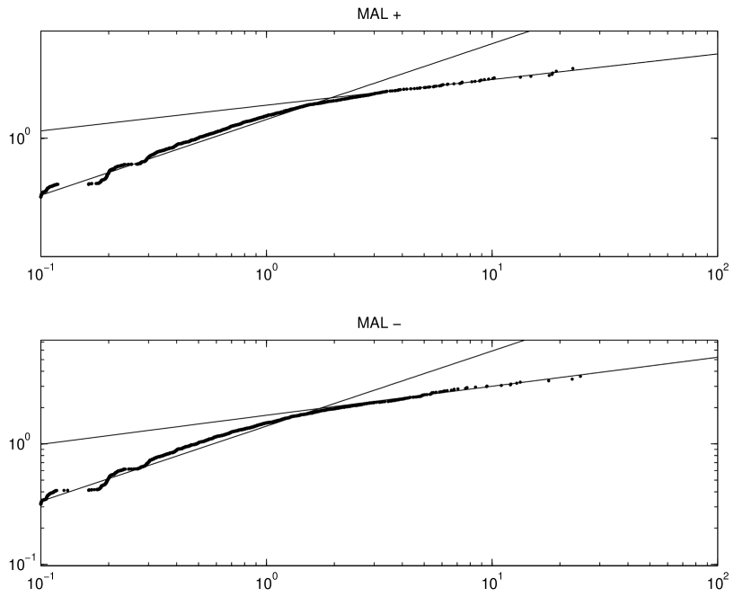
Figure 8: Graph of Gaussianized Malaysian Ringgit returns versus Malaysian Ringgit returns, for the time interval from Jan. 1971 to Oct. 1998. The upper graph gives the positive tail and the lower one the negative tail. The two straight lines represent the curves $y=\sqrt{2}\left(\frac{x}{\langle\chi_{\pm}\rangle}\right)^{\langle c_{\pm}\rangle}$ and $y=\sqrt{2}\left(\frac{x}{\chi_{\pm}}\right)^{c_{\pm}}$

In order to test the validity of our assumption, we have studied a large basket of financial assets including currencies and stocks. As an example, we present in figures 8 to 12 typical log-log plot of the transformed return variable $Y$ versus the return variable $X$ for a certain number of assets. If our assumption was right, we should observe a single straight line whose slope is given by $c/2$. In contrast, we observe in general two approximately linear regimes separated by a cross-over. This means that the marginal distribution of returns can be approximated by two modified Weibull distributions, one for small returns which is close to a Gaussian law and one for large returns with a fat tail. Each regime is depicted by its corresponding straight line in the graphs. The exponents $c$ and the scale factors $\chi$ for the different assets we have studied are given in tables 1 for currencies and 2 for stocks. The coefficients within brackets are the coefficients estimated for small returns while the non-bracketed coefficients correspond to the second fat tail regime.

The first point to note is the difference between currencies and stocks. For small as well as for large returns, the exponents $c_{-}$ and $c_{+}$ for currencies (excepted Poland and Thailand) are all close to each other. Additional tests are required to establish whether their relatively small differences are statistically significant. Similarly, the scale factors are also comparable. In contrast, many stocks exhibit a large asymmetric behavior for large returns with $c_{+}-c_{-}\gtrsim 0.5$ in about one-half of the investigated stocks. This means that the tails of the large negative returns (“crashes”) are often much fatter than those of the large positive returns (“rallies”).

The second important point is that, for small returns, many stocks have an exponent $\langle c_{+}\rangle\approx\langle c_{-}\rangle\simeq 2$ and thus have a behavior not far from a pure Gaussian, while the average exponent for currencies is about $1.5$ in the same “small return” regime. Therefore, even for small returns, currencies exhibit a strong departure from Gaussian behavior.

In conclusion, this empirical study shows that the modified Weibull parameterization, although not exact on the entire range of variation of the returns $X$, remains consistent within each of the two regimes of small versus large returns, with a sharp transition between them. It seems especially relevant in the tails of the return distributions, on which we shall focus our attention next.

4 Asymptotic estimation of the Value-at-Risk

Here, we examine theoretically the tail of the distribution of returns of portfolios constituted of assets with distributions characterized by the modified Weibull distributions. Two distinct situations can occur.

• The tail exponents $c$ of the distributions of asset returns are different from asset to asset. This is the most general case and at the same time the simplest. When the assets have different exponent $c$, the asymptotic tails of the portfolio return distribution are dominated by the asset with the heaviest tails. The largest risks of the portfolio are thus controlled by the single most risky asset characterized by the smallest exponent $c$. Such extreme risk cannot be diversified away. The best strategy focused on minimizing the extreme risks in such a case consists in holding only the asset with the thinnest tail, i.e., with the large exponent $c$.

• All assets in the portfolio have the same tail exponent $c$. This case is the most interesting and challenging as we shall see. We now present general asymptotic results for this case.

4.1 Portfolio made of assets with the same exponent $c>1$

4.1.1 Case of independent assets

Consider $N$ assets caracterized by their returns $X_{i}$, $i=\{1,2,\cdots,N\}$, with joint distribution $P({\bf x})$. We have seen in the first section that the portfolio return $S$ can be written as

$$S=\sum_{i=1}^{N}w_{i}X_{i}\;,$$ (31)

where the weights $w_{i}$ are real coefficients. The variables $\{X_{i}\}$ may be subjected to several constraints. Then, the probability density $P_{S}$ of the random variable $S$ is given by

$$P(S)=\int dx_{1}\cdots dx_{n}P(x_{1},\cdots,x_{N})~{}\delta\left(\sum w_{i}x_{i}-S\right)~{},$$ (32)

where $\delta$ is the Dirac function. Our purpose here is to evaluate its asymptotic behavior in the case where

$$P(x_{1},\cdots,x_{N})=P_{1}(x_{1})\cdots P_{N}(x_{N})~{}.$$ (33)

Using a saddle point approximation (see appendix A), we show that for large $S$:

$$P(S)\sim\left[\frac{c^{\frac{N+1}{2}}}{\chi~{}2^{\frac{N+1}{2}}(c-1)^{\frac{N-1}{2}}}\prod_{i=1}^{N}(w_{i}\chi_{i})^{\frac{c-1}{2}+\frac{1}{2(c-1)}}\right]~{}\left(\frac{|S|}{\chi}\right)^{c-2}e^{-\left(\frac{|S|}{\chi}\right)^{c}}~{},$$ (34)

where $\chi$ is given by

$$\chi^{\frac{c}{c-1}}=\sum_{i=1}^{N}(w_{i}\chi_{i})^{\frac{c}{c-1}}~{}.$$ (35)

Thus, for a large enough $VaR$ or equivalently for a small enough loss probability,

$$\Pr\{S<-VaR\} \simeq \frac{c^{\frac{N+1}{2}}}{\chi~{}2^{\frac{N+1}{2}}(c-1)^{\frac{N-1}{2}}}\prod_{i=1}^{N}(w_{i}\chi_{i})^{\frac{c-1}{2}+\frac{1}{2(c-1)}}\int_{-\infty}^{-{\rm VaR}}dS~{}\left(\frac{|S|}{\chi}\right)^{c-2}e^{-\left(\frac{|S|}{\chi}\right)^{c}}$$ (36)

$$\simeq \frac{c^{\frac{N-1}{2}}}{2^{\frac{N+1}{2}}(c-1)^{\frac{N-1}{2}}}\prod_{i=1}^{N}(w_{i}\chi_{i})^{\frac{c-1}{2}+\frac{1}{2(c-1)}}~{}\Gamma\left(\frac{c-1}{c},\left(\frac{VaR}{\chi}\right)^{c}\right)~{},$$ (37)

where $\Gamma(\cdot,\cdot)$ is the incomplet Gamma function. Using an asymptotic expansion of the incomplet gamma function, this finally yields

$$\Pr\{S<-VaR\}\simeq\left[\frac{c^{\frac{N-1}{2}}}{2^{\frac{N+1}{2}}(c-1)^{\frac{N-1}{2}}}\prod_{i=1}^{N}(w_{i}\chi_{i})^{\frac{c-1}{2}+\frac{1}{2(c-1)}}\right]~{}\frac{\exp\left[-\left(\frac{VaR}{\chi}\right)^{c}\right]}{\left(\frac{VaR}{\chi}\right)}$$ (38)

Our result here recover the previously announced [26] asymptotic form $e^{-\left(\frac{|S|}{\chi}\right)^{c}}$ for the tail of the distribution but corrects an error in the calculation of the characteristic scale $\chi$.

4.1.2 Case of dependent assets

We now consider the case of dependent assets with pdf given by equation (30) or its asymmetric expression. The calculation performed in appendix A leads to the following asymptotic expression for the density function $P(S)$ for large portfolio returns $S$ :

$$P(S)\propto\left(\frac{|S|}{\chi}\right)^{2-c}~{}e^{-\left(\frac{S}{\chi}\right)^{c}}~{},$$ (39)

and the following asymptotic $VaR$ :

$$\Pr\{S<-VaR\}\simeq C^{st}~{}\Gamma\left(\frac{c-1}{c},\left(\frac{VaR}{\chi}\right)^{c}\right)~{},$$ (40)

where $C^{st}$ is a term independent of $S$, whose expression is given appendix A and $\chi$ is such that

$$\chi^{c}=\frac{1}{c\sum_{i,j}V_{ij}^{-1}\sigma_{i}^{c/2}\sigma_{j}^{c/2}}~{},$$ (41)

and the $\{\sigma_{i}\}$ are solution of

$$\sum_{i}V_{ik}^{-1}\sigma_{i}^{c/2}\sigma_{k}^{c/2}=w_{k}\chi_{k}\sigma_{k}~{}\sum_{i,j}V_{ij}^{-1}\sigma_{i}^{c/2}\sigma_{j}^{c/2}~{}.$$ (42)

Obviously, if the assets are independent, $V_{ij}^{-1}=\delta_{ij}$, the $\sigma_{i}$’s are solution of

$$\sigma_{i}^{c-1} = \lambda w_{i}\chi_{i},~{}~{}\forall i\in\{1,\cdots,N\}$$ (43)

$$\lambda = \sum_{i}\sigma_{i}^{c}~{},$$ (44)

$\chi$ is then simply given by equation (35).

4.2 Portfolio made of assets with the same exponent $c<1$

In the case of independent assets whose tails of distributions are fatter than an exponential, the tail of the distribution of price variations of the portfolio is given by [26]

$$P(S)\sim\exp\left[-\left(\frac{|S|}{\chi}\right)^{c}\right]\;,$$ (45)

with

$$\chi^{2}=\max_{i\in\{1,..N\}}\{w_{1}^{2}\chi_{1}^{2},\cdots,w_{N}^{2}\chi_{N}^{2}\}~{}.$$ (46)

This single variable $\chi$ controls the asymptotic behavior of the tail of the distribution.

Using the equation (45), the Value-at-Risk is solution of

$$\Pr\{S<-VaR\}\sim\int_{-\infty}^{-{\rm VaR}}dS~{}e^{-\left(\frac{|S|}{\chi}\right)^{c}}~{},$$ (47)

i.e :

$$\Pr\{S<-VaR\}\sim\Gamma\left(\frac{1}{c},{\rm VaR}^{c}\right)~{}.$$ (48)

In the case of correlated assets, we have not yet found an asymptotic formula. But, using the standard result that a sum of stretched exponentially distributed random variables behaves, in the regime of large deviation, like the variable whose deviation is the most extreme, we expect the previous result to remain true.

4.3 Summary

In summary, the density function $P(S)$ behaves for large $S$ like

$$P(S)\sim e^{-\left(\frac{|S|}{\chi}\right)^{c}}~{},$$ (49)

where

$$\chi = \left(\sum_{i}(w_{i}\chi_{i})^{\frac{c}{c-1}}\right)^{\frac{c-1}{c}}~{}~{}\mbox{if }~{}c>1~{}~{}\mbox{ and~{} independent~{} assets}~{},$$ (50)

$$\chi = \frac{1}{\left(c\sum_{i,j}V_{ij}^{-1}\sigma_{i}^{c/2}\sigma_{j}^{c/2}\right)^{\frac{1}{c}}}~{}~{}\mbox{if}~{}c>1~{}~{}\mbox{ and~{} dependent~{} assets}~{},$$ (51)

$$\chi = \left(\max_{i\in\{1,..N\}}\{w_{1}^{2}\chi_{1}^{2},\cdots,w_{N}^{2}\chi_{N}^{2}\}\right)^{1/2}~{}~{}\mbox{if }~{}c<1~{}.$$ (52)

Note that the expression (50) for $c>1$ retrieves the result (52) for $c<1$ by taking the limit $c\to 1^{+}$, showing the continuity of the formulas.

Let us translate these formulas in intuitive form. For this, we define a value-at-risk (VaR) $VaR^{*}$ which is such that its typical frequency is $1/T_{0}$. $T_{0}$ is by definition the typical recurrence time of a loss larger than $VaR^{*}$. In our present example, we take $T_{0}$ equals $1$ year for example, i.e., $VaR^{*}$ is the typical annual shock or crash. The expression (49) then allows us to predict the recurrence time $T$ of a VaR equal to $\alpha$ times this reference value $VaR^{*}$:

$$\ln\left(\frac{T}{T_{0}}\right)\simeq(\alpha^{c}-1)\left(\frac{VaR^{*}}{\chi}\right)^{c}+{\cal O}(\ln\alpha)~{}.$$ (53)

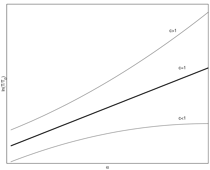
Figure 13: Logarithm $\ln\left(\frac{T}{T_{0}}\right)$ of the ratio of the recurrence time $T$ to a reference time $T_{0}$ for the recurrence of a given loss $VaR$ as a function of $\alpha$ defined by $\alpha=\frac{VaR}{VaR^{*}}$. $VaR^{*}$ (resp. $VaR$) is the Value-at-Risk over a time interval $T_{0}$ (resp. $T$).

Figure 13 shows $\ln\frac{T}{T_{0}}$ versus $\alpha$. For fixed $\alpha$, $T$ increases more and more slowly when the exponent $c$ decreases. This quantifies our expectation that large losses occur more frequently for sub-exponential distributions than for super-exponential ones.

5 Cumulant expansion of the portfolio return distribution

5.1 link between moments and cumulants

Before deriving the main result of this section, we recall a standard relation between moments and cumulants that we need below.

The moments $M_{n}$ of the distribution $P$ are defined by

$$\hat{P}(k)=\sum_{n=0}^{+\infty}\frac{(ik)^{n}}{n!}M_{n}~{},$$ (54)

where $\hat{P}$ is the characteristic function, i.e., the Fourier transform of $P$ :

$$\hat{P}(k)=\int_{-\infty}^{+\infty}dS~{}P(S)e^{ikS}~{}.$$ (55)

Similarly, the cumulants $C_{n}$ are given by

$$\hat{P}(k)=\exp\left(\sum_{n=1}^{+\infty}\frac{(ik)^{n}}{n!}C_{n}\right)~{}.$$ (56)

Differentiating $n$ times the equation

$$\ln\left(\sum_{n=0}^{+\infty}\frac{(ik)^{n}}{n!}M_{n}\right)=\sum_{n=1}^{+\infty}\frac{(ik)^{n}}{n!}C_{n}\;,$$ (57)

we obtain the following recurrence relations between the moments and the cumulants :

$$M_{n} = \sum_{p=0}^{n-1}{{n-1}\choose{p}}M_{p}C_{n-p}\;,$$ (58)

$$C_{n} = M_{n}-\sum_{p=1}^{n-1}{{n-1}\choose{n-p}}C_{p}M_{n-p}\;.$$ (59)

In the sequel, we will first evaluate the moments, which turns out to be easier, and then using eq (59) we will be able to calculate the cumulants. Cumulants are indeed the natural objects to quantify risks: as seen from their definition (56), cumulants of order larger than $2$ quantify deviation from the Gaussian law, and thus large risks beyond the variance (equal to the second-order cumulant). More importantly, they are invariant with respect to translations or change of a return of reference and are thus appropriate measures of fluctuations.

5.2 Symmetric assets

We start with the expression (32) of the distribution of the weighted sum of $N$ assets :

$$P_{S}(s)=\int_{R^{N}}d{\bf x}\;P({\bf x})\delta(\sum_{i=1}^{N}w_{i}x_{i}-s)\;.$$ (60)

Using the change of variable (12), allowing us to go from the asset returns $X_{i}$’s to the transformed returns $Y_{i}$’s, we get

$$P_{S}(s)=\frac{1}{(2\pi)^{N/2}\sqrt{\det(V)}}\int_{R^{N}}d{\bf y}\;e^{-\frac{1}{2}{\bf y^{t}}V^{-1}{\bf y}}\;\delta(\sum_{i=1}^{N}w_{i}sgn(y_{i})f^{-1}(y_{i}^{2})-s)\;.$$ (61)

Taking its Fourier transform $\hat{P}_{S}(k)=\int dsP_{S}(s)e^{iks}$, we obtain

$$\hat{P}_{S}(k)=\frac{1}{(2\pi)^{N/2}\sqrt{\det(V)}}\int_{R^{N}}d{\bf y}\;e^{-\frac{1}{2}{\bf y^{t}}V^{-1}{\bf y}+ik\sum_{i=1}^{N}w_{i}sgn(y_{i})f^{-1}(y_{i}^{2})}\;,$$ (62)

where $\hat{P}_{S}$ is the characteristic function of $P_{S}$.

In the particular case of interest here where the marginal distributions of the variables $X_{i}$’s are the modified Weibull pdf,

$$f^{-1}(y_{i})=\chi_{i}|\frac{y_{i}}{\sqrt{2}}|^{q_{i}}$$ (63)

with

$$q_{i}=2/c_{i}~{},$$ (64)

the equation (62) becomes

$$\hat{P}_{S}(k)=\frac{1}{(2\pi)^{N/2}\sqrt{\det(V)}}\int_{R^{N}}d{\bf y}\;e^{-\frac{1}{2}{\bf y^{t}}V^{-1}{\bf y}+ik\sum_{i=1}^{N}w_{i}sgn(y_{i})\chi_{i}|\frac{y_{i}}{\sqrt{2}}|^{q_{i}}}\;.$$ (65)

The task in front of us is to evaluate this expression through the determination of the moments and/or cumulants.

5.2.1 Case of independent assets

In this case, the cumulants can be obtained explicitely [26]. Indeed, the expression (65) can be expressed as a product of integrals of the form

$$\int_{0}^{+\infty}du\;e^{-\frac{u^{2}}{2}+ikw_{i}\chi_{i}\left(\frac{u}{\sqrt{2}}\right)^{q_{i}}}\;.$$ (66)

We obtain

$$C_{2n}=\sum_{i=1}^{N}c(n,q_{i})(\chi_{i}w_{i})^{2n}\;,$$ (67)

and

$$c(n,q_{i})=(2n)!\left\{\sum_{p=0}^{n-2}(-1)^{n}\frac{\Gamma\left(q_{i}(n-p)+\frac{1}{2}\right)}{(2n-2p)!\pi^{1/2}}\left[\frac{\Gamma\left(q_{i}+\frac{1}{2}\right)}{2!\pi^{1/2}}\right]^{p}-\frac{(-1)^{n}}{n}\left[\frac{\Gamma\left(q_{i}+\frac{1}{2}\right)}{2!\pi^{1/2}}\right]^{n}\right\}\;.$$ (68)

Note that the coefficient $c(n,q_{i})$ is the cumulant of order $n$ of the marginal distribution (24) with $c=2/q_{i}$ and $\chi=1$. The equation (67) expresses simply the fact that the cumulants of the sum of independent variables is the sum of the cumulants of each variable. The odd-order cumulants are zero due to the symmetry of the distributions.

5.2.2 Case of dependent assets

Here, we restrict our exposition to the case of two random variables. The case with $N$ arbitrary can be treated in a similar way but involves rather complex formulas. The equation (65) reads

$$\hat{P}_{S}(k)=\frac{1}{2\pi\sqrt{1-\rho^{2}}}\int dy_{1}dy_{2}~{}\exp\left[-\frac{1}{2}y^{t}V^{-1}y+ik\left(\chi_{1}w_{1}sgn(y_{1})\left|\frac{y_{1}}{\sqrt{2}}\right|^{q_{1}}+\right.\right.{}$$

$$\left.\left.+\chi_{2}w_{2}sgn(y_{2})\left|\frac{y_{2}}{\sqrt{2}}\right|^{q_{2}}\right)\right]~{},$$ (69)

and we can show (see appendix B) that the moments read

$$M_{n}=\sum_{p=0}^{n}{n\choose p}w_{1}^{p}w_{2}^{n-p}\gamma_{q_{1}q_{2}}(n,p)~{},$$ (70)

with

$$\gamma_{q_{1}q_{2}}(2n,2p) = \chi_{1}^{2p}\chi_{2}^{2(n-p)}\frac{\Gamma\left(q_{1}p+\frac{1}{2}\right)\Gamma\left(q_{2}(n-p)+\frac{1}{2}\right)}{\pi}~{}{{}_{2}F_{1}}\left(-q_{1}p,-q_{2}(n-p);\frac{1}{2};\rho^{2}\right)\;,$$ (71)

$$\gamma_{q_{1}q_{2}}(2n,2p+1) = 2\chi_{1}^{2p+1}\chi_{2}^{2(n-p)-1}\frac{\Gamma\left(q_{1}p+1+\frac{q_{1}}{2}\right)\Gamma\left(q_{2}(n-p)+1-\frac{q_{2}}{2}\right)}{\pi}\rho~{}{{}_{2}F_{1}}\left(-q_{1}p-\frac{q_{1}-1}{2},\right.$$ (72)

$$\left.,-q_{2}(n-p)+\frac{q_{2}+1}{2};\frac{3}{2};\rho^{2}\right)~{},$$

where ${{}_{2}F_{1}}$ is an hypergeometric function.

These two relations allow us to calculate the moments and cumulants for any possible values of $q_{1}=2/c_{1}$ and $q_{2}=2/c_{2}$. If one of the $q_{i}$’s is an integer, a simplification occurs and the coefficients $\gamma(n,p)$ reduce to polynomials. In the simpler case where all the $q_{i}$’s are odd integer the expression of moments becomes :

$$M_{n}=\sum_{p=0}^{n}{n\choose p}\left(w_{1}{\chi_{1}}\right)^{p}\left(w_{2}{\chi_{2}}\right)^{n-p}\sum_{s=0}^{min\{q_{1}p,q_{2}(n-p)\}}{\rho}^{s}~{}s!~{}a_{s}^{(q_{1}p)}a_{s}^{(q_{2}(n-p))}~{},$$ (73)

with

$$a_{2p}^{(2n)} = (2p)!C_{2n}^{2(n-p)}(2(n-p)-1)!!=\frac{(2n)!}{2^{(2n-2p)}(2p)!(n-p)!}\;,$$ (74)

$$a_{2p+1}^{(2n)} = 0\;,$$ (75)

$$a_{2p}^{(2n+1)} = 0\;,$$ (76)

$$a_{2p+1}^{(2n+1)} = (2p+1)!C_{2n+1}^{2(n-p)}(2(n-p)-1)!!=\frac{(2n+1)!}{2^{(2n-2p)}(2p+1)!(n-p)!}\;,$$ (77)

5.3 Non-symmetric assets

In the case of asymmetric assets, we have to consider the formula (25-26), and using the same notation as in the previous section, the moments are again given by (70) with the coefficient $\gamma(n,p)$ now equal to :

$$\gamma(n,p)=\frac{(-1)^{n}(\chi_{1}^{-})^{p}(\chi_{2}^{-})^{n-p}}{4\pi}\left[\Gamma\left(\frac{q_{1}^{-}p+1}{2}\right)\Gamma\left(\frac{q_{2}^{-}(n-p)+1}{2}\right)~{}_{2}F_{1}\left(-\frac{q_{1}^{-}p}{2},-\frac{q_{2}^{-}(n-p)}{2};\frac{1}{2};\rho^{2}\right)+\right.$$

$$\left.+2\Gamma\left(\frac{q_{1}^{-}p}{2}+1\right)\Gamma\left(\frac{q_{2}^{-}(n-p)}{2}+1\right)\rho~{}_{2}F_{1}\left(-\frac{q_{1}^{-}p-1}{2},-\frac{q_{2}^{-}(n-p)-1}{2};\frac{3}{2};\rho^{2}\right)\right]+$$

$$+\frac{(-1)^{p}(\chi_{1}^{-})^{p}(\chi_{2}^{+})^{n-p}}{4\pi}\left[\Gamma\left(\frac{q_{1}^{-}p+1}{2}\right)\Gamma\left(\frac{q_{2}^{+}(n-p)+1}{2}\right)~{}_{2}F_{1}\left(-\frac{q_{1}^{-}p}{2},-\frac{q_{2}^{+}(n-p)}{2};\frac{1}{2};\rho^{2}\right)+\right.$$

$$\left.-2\Gamma\left(\frac{q_{1}^{-}p}{2}+1\right)\Gamma\left(\frac{q_{2}^{+}(n-p)}{2}+1\right)\rho~{}_{2}F_{1}\left(-\frac{q_{1}^{-}p-1}{2},-\frac{q_{2}^{+}(n-p)-1}{2};\frac{3}{2};\rho^{2}\right)\right]+$$

$$+\frac{(-1)^{n-p}(\chi_{1}^{+})^{p}(\chi_{2}^{-})^{n-p}}{4\pi}\left[\Gamma\left(\frac{q_{1}^{+}p+1}{2}\right)\Gamma\left(\frac{q_{2}^{-}(n-p)+1}{2}\right)~{}_{2}F_{1}\left(-\frac{q_{1}^{+}p}{2},-\frac{q_{2}^{-}(n-p)}{2};\frac{1}{2};\rho^{2}\right)+\right.$$

$$\left.-2\Gamma\left(\frac{q_{1}^{+}p}{2}+1\right)\Gamma\left(\frac{q_{2}^{-}(n-p)}{2}+1\right)\rho~{}_{2}F_{1}\left(-\frac{q_{1}^{+}p-1}{2},-\frac{q_{2}^{-}(n-p)-1}{2};\frac{3}{2};\rho^{2}\right)\right]+$$

$$+\frac{(\chi_{1}^{+})^{p}(\chi_{2}^{+})^{n-p}}{4\pi}\left[\Gamma\left(\frac{q_{1}^{+}p+1}{2}\right)\Gamma\left(\frac{q_{2}^{+}(n-p)+1}{2}\right)~{}_{2}F_{1}\left(-\frac{q_{1}^{+}p}{2},-\frac{q_{2}^{+}(n-p)}{2};\frac{1}{2};\rho^{2}\right)+\right.$$

$$\left.+2\Gamma\left(\frac{q_{1}^{+}p}{2}+1\right)\Gamma\left(\frac{q_{2}^{+}(n-p)}{2}+1\right)\rho~{}_{2}F_{1}\left(-\frac{q_{1}^{+}p-1}{2},-\frac{q_{2}^{+}(n-p)-1}{2};\frac{3}{2};\rho^{2}\right)\right]~{}.$$

This formula is obtained in the same way as the formulas given in the symmetric case. We retrieve the formula (71) as it should if the coefficients ’+’ are equal to the coefficients ’-’.

5.4 Empirical tests

Extensive tests have been performed for currencies under the assumption that the distributions of asset returns are symmetric [26].

As an exemple, let us consider the Swiss franc and the Japanese Yen against the US dollar. The calibration of the modified Weibull distribution to the tail of the empirical histogram of daily returns give $(q_{CHF}=1.75,c_{CHF}=1.14,\chi_{CHF}=2.13)$ and $(q_{JPY}=2.50,c_{JPY}=0.8,\chi_{JPY}=1.25)$ and their correlation coefficient is $\rho=0.43$.

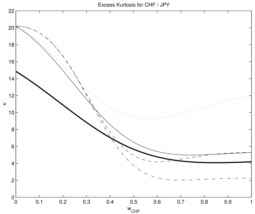
Figure 14: Excess kurtosis of the distribution of the price variation $w_{CHF}x_{CHF}+w_{JPY}x_{JPY}$ of the portfolio made of a fraction $w_{CHF}$ of Swiss franc and a fraction $w_{JPY}=1-w_{CHF}$ of the Japanese Yen against the US dollar, as a function of $w_{CHF}$, denoted $w$ in the figure. Thick solid line : empirical curve, thin solid line : theoretical curve, dashed line : theoretical curve with $\rho=0$ (instead of $\rho=0.43$), dotted line: theoretical curve with $q_{CHF}=2$ rather than $1.75$ and dashed-dotted line: theoretical curve with $q_{CHF}=1.5$. The excess kurtosis has been evaluated for the time interval from Jan. 1971 to Oct. 1998.

The figure 14 plots the excess kurtosis of the sum $w_{CHF}x_{CHF}+w_{JPY}x_{JPY}$ as a function of $w_{CHF}$, denoted $w$ in the figure, with the “no-short” constraint $w_{CHF}+w_{JPY}=1$. The thick solid line is determined empirically, by direct calculation of the kurtosis from the data. The thin solid line is the theoretical prediction using our theoretical formulas with the empirically determined exponents $c$ and characteristic scales $\chi$ given above. While there is a non-negligible difference, the empirical and theoretical excess kurtosis have essentially the same behavior with their minimum reached almost at the same value of $w_{CHF}$.

Three origins of the discrepancy between theory and empirical data can be invoked. First, as already pointed out in the preceding section, the modified Weibull distribution with constant exponent and scale parameters describes accurately only the tail of the empirical distributions while, for small returns, the empirical distributions are close to a Gaussian law. While putting a strong emphasis on large fluctuations, cumulants of order $4$ are still significantly sensitive to the bulk of the distributions. Moreover, the excess kurtosis is normalized by the square second-order cumulant, which is almost exclusively sensitive to the bulk of the distribution. Cumulants of higher order should thus be better described by the modified Weibull distribution. However, a careful comparison between theory and data would then be hindered by the difficulty in estimating reliable empirical cumulants of high order. The second possible origin of the discrepancy between theory and data is the existence of a weak asymmetry of the empirical distributions, particularly of the Swiss franc, which has not been taken into account. The figure also suggests that an error in the determination of the exponents $c$ can also contribute to the discrepancy.

In order to study investigate the sensitivity with respect to the choice of the parameters $q$ and $\rho$, we have also constructed the dashed line corresponding to the theoretical curve with $\rho=0$ (instead of $\rho=0.43$) and the dotted line corresponding to the theoretical curve with $q_{CHF}=2$ rather than $1.75$. Finally, the dashed-dotted line corresponds to the theoretical curve with $q_{CHF}=1.5$. We observe that the dashed line remains rather close to the thin solid line while the dotted line departs significantly when $w$ increases. Therefore, the most sensitive parameter is $q$, which is natural because it controls directly the extend of the fat tail of the distributions.

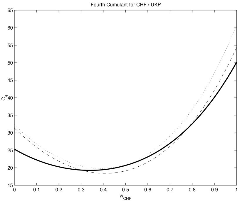
Figure 15: Fourth cumulant for a portfolio made of a fraction $w_{CHF}$ of Swiss Franc and $1-w_{CHF}$ of British Pound. The thick solid line represents the empirical cumulant while the dotted line represents the theoretical cumulant under the symmetric assumption. The dashed line shows the theoretical cumulant when the slight asymmetry of the assets has been taken into account. This cumulant has been evaluated for the time interval from Jan. 1971 to Oct. 1998.

In order to account for the effect of asymmetry, we have plotted the fourth cumulant of a portfolio compound of Swiss Franc and British Pound. On figure 15, the solid line represents the empirical cumulant while the dashed line shows the theorical cumulant. The agreement between the two curves is better than under the symmetric asumption. Note once again that an accurate determination of the parameters is the key point to obtain a good agreement between empirical data and theoretical prediction. As we can see in the figure 15, the paramaters of the Swiss Franc seem well adjusted since the theoretical and empirical cumulants are both very close when $w\simeq 1$, i.e., when the Swiss Franc is almost the sole asset in the portfolio, while when $w\simeq 0$, the theorical cumulant is far from the empirical one, i.e., the parameters of the Bristish Pound are not sufficiently well-adjusted.

6 Portfolio optimization

Up to now, we have calculated several measures of risk: the asymptotic distribution of losses and the corresponding Value-at-Risk to quantify the large fluctuations and the cumulants to evaluate smaller fluctuations. We now present different strategies of portfolio allocation constructed using these risk measures.

6.1 Optimization with respect to the Value-at-Risk

As already said, in the case of assets with different exponent $c$, there is no possible diversification of large risks. Therefore, the strategy minimizing large risks consists in holding as little as possible of the more fat-tailed assets, compatible with the constraint on the average return of the portfolio. Obviously, if only large risk control matters, one should only hold the asset with the thinnest tail.

The more interesting case occurs when the exponents $c$ are the same for the different assets of the portfolio. According to the tables 1 and 2, this is indeed an relevant situation, when taking into account the error bars in the exponents. It is then easy to show, from the results given in section 4, that the VaR is an increasing function of the scale parameter $\chi$ where:

$$\chi^{c}=\frac{1}{c\sum_{i,j}V_{ij}^{-1}\sigma_{i}^{c/2}\sigma_{j}^{c/2}}$$ (79)

when $c>1$ and

$$\chi^{2}=\max_{i\in\{1,..N\}}\{w_{1}^{2}\chi_{1}^{2},\cdots,w_{N}^{2}\chi_{N}^{2}\}$$ (80)

if $c\leq 1$.

Thus, the optimization program to fulfill is :

$$\left\{\begin{array}[]{l}{\chi^{*}}\equiv\inf_{\{w_{i}\}}{\rm VaR}(\{w_{i}\})\\ \sum_{i}w_{i}=1\\ \sum_{i}w_{i}\mu_{i}=\mu\end{array}\right.$$ (81)

where $\mu_{i}$ denotes the average return of asset $i$ and $\mu$ the average return of the portfolio.

Case $c>1$ :

In the case, we can give the analytical form of the efficient frontier, i.e., $\mu$ versus ${\chi^{*}}^{c}$ (at least) in the independent case. Let $\lambda_{1}$ and $\lambda_{2}$ denote two Langrange multipliers. We have to solve

$$\frac{\partial}{\partial w_{k}}\left(\chi-\lambda_{1}\left(\sum_{i}w_{i}-1\right)-\lambda_{2}\left(\sum_{i}w_{i}\mu_{i}\right)\right)=0~{},$$ (82)

which leads to

$$\left(\sum_{i}(w_{i}^{*}\chi_{i})^{\frac{c}{c-1}}\right)^{\frac{c-1}{c}-1}\chi_{k}^{\frac{c}{c-1}}{w_{k}^{*}}^{\frac{c}{c-1}-1}=\lambda_{1}+\lambda_{2}\mu_{k}~{}.$$ (83)

Multiplying by $w_{k}^{*}$ and summing over $k$, we obtain :

$$\lambda_{1}+\lambda_{2}\mu=\chi~{}.$$ (84)

Then, expressing $w_{k}^{*}$ from eq.(83) and accounting for the constraint, we obtain an analytical parametric equation of the efficient frontier :

$$\left\{\begin{array}[]{l}\sum_{i}\frac{(\lambda_{1}+\lambda_{2}\mu_{i})^{c-1}}{\chi_{i}^{c}}=\chi^{*}\\ \sum_{i}\frac{\mu_{i}(\lambda_{1}+\lambda_{2}\mu_{i})^{c-1}}{\chi_{i}^{c}}=\mu\chi^{*}\\ \lambda_{1}+\lambda_{2}\mu=\chi^{*}\end{array}\right.$$ (85)

Varying $\lambda_{1}$ and $\lambda_{2}$, the efficient frontier is delineated. In the Gaussian case $c=2$, we retrieve the standard Markovitz efficient frontier.

In the case of correlated assets, the shape of the frontier remains essentially the same but its determination requires numerical calculation.

Case $c<1$ :

In this case, the general minimization problem must be again solve numerically. As an example, we consider the simple case where the portfolio is made of only two assets. This case is analyticaly soluble. Indeed, the program

$$\left\{\begin{array}[]{l}\inf_{w^{*}\in[0,1]}\{\sup_{i\in\{1,..N\}}\{w_{1}^{2}\chi_{1}^{2},\cdots,w_{N}^{2}\chi_{N}^{2}\}\}\\ \sum_{i}w_{i}=1\\ \sum_{i}w_{i}\mu_{i}=\mu\end{array}\right.$$ (86)

simplifies into :

$$\inf_{\mu\in[\mu_{1},\mu_{2}]}\left\{\sup\left\{\left(\frac{\mu-\mu_{2}}{\mu_{1}-\mu_{2}}\right)^{2}\chi_{1}^{2},\left(\frac{\mu_{1}-\mu}{\mu_{1}-\mu_{2}}\right)^{2}\chi_{2}^{2}\right\}\right\}\;.$$ (87)

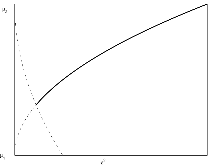
Figure 16: Efficient frontier (thick line) in the case of two assets with the same exponent lower than $1$.

The thick line on figure 16 represents the efficient frontier while the dashed lines represent $\mu=f(\chi_{1})$ and $\mu=f(\chi_{2})$.

6.2 Optimization with respect to the cumulants

A priori, all order cumulants can be considered and each of them embodies a certain measure of risk. Obviously, the larger the cumulant order, the more sensitive is the cumulant to large fluctuations. We can expect risk control based on the high-order cumulants will be equivalent to risk-control based on the VaR approach [26]. In this section, we will only focus on relatively low-order cumulants, because they are expected to add valuable information on top of the risk structure already provided by the VaR approach. By lower-order, we mean cumulants of order $n=2$ to $n=6$. To justify this approach, we have evaluated the cumulants for several portfolios and it is very clear that, in most cases for $n>6$, they become strictly monotonous functions of the asset weights within the interval $[0,1]^{N}$. Therefore, the minimization of risks which would correspond to minimizing cumulants of order larger than $n=6$ would lead once more to hold as little as possible of the more fat-tailed assets.

The portfolio optimization along the lines of [26, 25, 2] corresponds to minimizing a given cumulant $C_{n}$ of order $n$ of the distribution of returns of the portfolio in the presence of a constraint on the return as well as the “no-short” constraint:

$$\left\{\begin{array}[]{l}\inf_{w_{i}\in[0,1]}C_{n}(\{w_{i}\})\\ \sum_{i}w_{i}=1\\ \sum_{i}w_{i}\mu_{i}=\mu~{}.\end{array}\right.$$ (88)

In the most general case, we have to use extentions for $N>2$ of the formulae given in section 5 and perform a numerical optimization. Interesting results can be observed in simpler situations, as we now obtain.

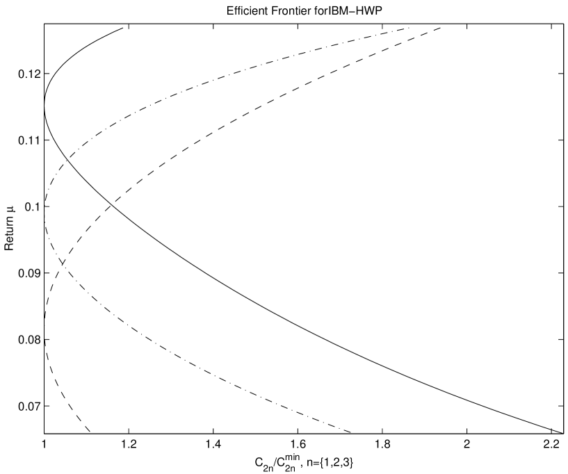
Figure 17: Efficient frontier for a portfolio composed of two stocks: IBM and Hewlett-Packard. The dashed line represents the efficient frontier with respect to the second cumulant, i.e., the standard Markovitz efficient frontier, the dash-doted line represents the efficient frontier with respect to the fourth cumulant and the solid line the efficient frontier with respect to the sixth cumulant. The data set used covers the time interval from Jan. 1977 to Dec 2000.

Figure 17 and 18 show the generalized efficient frontiers using $C_{2}$ (Markovitz case), $C_{4}$ or $C_{6}$ as relevant measures of risks, for two portfolios composed of two stocks : IBM and Hewlett-Packard in the first case and IBM and Coca-Cola in the second case.

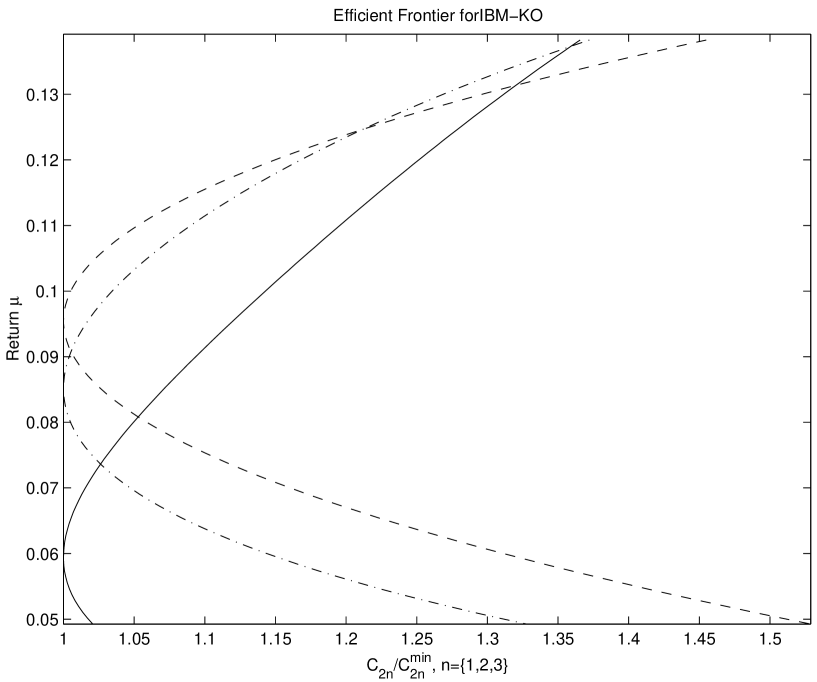
Figure 18: Efficient frontier for a portfolio composed of two stocks: IBM and Coca-Cola. The dashed line represents the efficient frontier with respect to the second cumulant,i.e., the standard Markovitz efficient frontier, the dash-doted line represents the efficient frontier with respect to the fourth cumulant and the solid line the efficient frontier with repect to the sixth cumulant. The dataset used covers the time interval from Jan. 1970 to Dec 2000.

Obviously, given a certain amount of risk, the mean return of the portfolio changes when the cumulant considered changes. It is interesting to note that, in figure 17, the minimisation of larger risks, i.e., with respect to $C_{6}$, increases the average return while, in figure 18, the minimisation of larger risk lead to decrease the average return.

This allows us to make precise and quantitative the previously reported empirical observation that it is possible to “have your cake and eat it too” [2]. We can indeed give a general criterion to determine under which values of the parameters (exponents $c$ and characteristic scales $\chi$ of the distributions of the asset returns) the average return of the portfolio may increase while the large risks decrease at the same time, thus allowing one to gain on both account (of course, the small risks quantified by the variance will then increase). For two independent assets, assuming that the cumulants of order $n$ and $n+k$ of the portfolio admit a minimum in the interval $]0,1[$, we can show that

$$\mu_{n}^{*}<\mu_{n+k}^{*}$$ (89)

if and only if

• $\mu_{1}-\mu_{2}>0$ and

  $$\left(\frac{C_{n}(1)}{C_{n}(2)}\right)^{\frac{1}{n-1}}>\left(\frac{C_{n+k}(1)}{C_{n+k}(2)}\right)^{\frac{1}{n+k-1}},$$ (90)

• $\mu_{1}-\mu_{2}<0$ and

  $$\left(\frac{C_{n}(1)}{C_{n}(2)}\right)^{\frac{1}{n-1}}<\left(\frac{C_{n+k}(1)}{C_{n+k}(2)}\right)^{\frac{1}{n+k-1}},$$ (91)

where $\mu_{n}^{*}$ denotes the return of the portfolio evaluated with respect to the minimum of the cumulant of order $n$ and $C_{n}(i)$ is the cumulant of order $n$ for the asset $i$.

The proof of this result and its generalisation to $N>2$ are given in appendix C. In fact, we have observed that when the exponent $c$ of the assets remains sufficiently different, this result still holds in presence of dependence between assets.

For the assets considered above, we have found $\mu_{IBM}=0.13$, $\mu_{HWP}=0.07$, $\mu_{KO}=0.05$ and

$$\frac{C_{2}(IBM)}{C_{2}(HWP)} =1.76>\left(\frac{C_{4}(IBM)}{C_{4}(HWP)}\right)^{\frac{1}{3}} =1.03>\left(\frac{C_{6}(IBM)}{C_{6}(HWP)}\right)^{\frac{1}{5}}=0.89$$ (92)

$$\frac{C_{2}(IBM)}{C_{2}(KO)} =0.96<\left(\frac{C_{4}(IBM)}{C_{4}(KO)}\right)^{\frac{1}{3}} =1.01<\left(\frac{C_{6}(IBM)}{C_{6}(KO)}\right)^{\frac{1}{5}}=1.06~{},$$ (93)

which shows that, for the portfolio IBM / Hewlett-Packard, the efficient return is an increasing function of the order of the cumulants while, for the portfolio IBM / Coca-Cola, the inverse phenomeon occurs. This is exactly what is shown on figures 17 and 18.

The underlying intuitive mechanism is the following: if a portfolio contains an asset with a rather fat tail (many “large” risks) but narrow waist (few “small” risks) with very little return to gain from it, minimizing the variance $C_{2}$ of the return portfolio will overweight this asset which is wrongly perceived as having little risk due to its small variance (small waist). In contrast, controlling for the larger risks quantified by $C_{4}$ or $C_{6}$ leads to decrease the weighing of this asset on the portfoio, and correspondingly to increase the weight of the more profitable assets. We thus see that the effect of “both decreasing large risks and increasing profit” appears when the asset(s) with the fatter tails, and therefore the narrower central part, has(ve) the smaller overall return(s). A mean-variance approach will weight them more than deemed appropriate from a prudential consideration of large risks and consideration of profits.

7 Conclusion

We have presented new analytical results on and empirical tests of a general framework for a portfolio theory of non-Gaussian risks with non-linear correlations. We have shown that the concept of efficient frontiers can be generalized by using other measures of risks than the variance (cumulant of order $2$), for instance the value-at-risk and the cumulants of order larger than $2$. This work opens several novel interesting avenues for research. One consists in extending the Gaussian copula assumption, for instance by using the maximum-entropy principle with non-extensive Tsallis entropies, known to be the correct mathematical information-theoretical representation of power laws. A second line of research would be to extend the present framework to encompass simultaneously different time scales $\tau$ in the spirit of [19] in the case of a cascade model of volatilities.

Appendix A Asymptotic expansion of the wealth distribution for a portfolio made of assets with same exponent $c$

A.1 Case of independent assets

We start with the definition $S=\sum_{i=1}^{N}w_{i}x_{i}$ and the corresponding equation for its probability density function :

$$P_{S}(S)\propto\int dx_{1}\cdots dx_{N}~{}e^{-\sum_{i=1}^{N}f_{i}(x_{i})}~{}\delta\left(S-\sum_{i=1}^{N}w_{i}x_{i}\right)~{},$$ (94)

where we have used the parameterization

$$P_{i}(x_{i})=C_{i}~{}e^{-f_{i}(x_{i})}~{},$$ (95)

and

$$f_{i}(x_{i})=\left(\frac{|x_{i}|}{\chi_{i}}\right)^{c}~{},~{}~{}\mbox{with c}>1~{}.$$ (96)

All equations in (94) are from $-\infty$ to $+\infty$. The delta function expresses the constraint on the sum. We need the following conditions on the functions $f_{i}$

• $f_{i}(x_{i})\rightarrow+\infty$ sufficiently fast to ensure the normalization of the pdf’s.

• $f_{i}^{\prime\prime}(x_{i})>0$ (convexity), where $f^{\prime\prime}$ denotes the second derivative of $f$.

• $\lim_{x\rightarrow\infty}x^{2}f(x)=+\infty$.

Under these assumptions, the leading order expansion of $P_{S}(S)$ for large $S$ and finite $N>1$ is obtained by a generalization of Laplace’s method which here amounts to remark that the set of $x_{i}^{*}$’s that maximize the integrand in (94) are solution of

$$f_{i}^{\prime}(x_{i}^{*})=\sigma(S)w_{i}~{},$$ (97)

where $\sigma(S)$ is nothing but a Lagrange multiplier introduced to minimize the expression $\sum_{i=1}^{N}f_{i}(x_{i})$ under the constraint $\sum_{i=1}^{N}w_{i}x_{i}=S$.

Expanding $f_{i}(x_{i})$ around $x_{i}^{*}$ yields

$$f_{i}(x_{i})=f_{i}(x_{i}^{*})+f_{i}^{\prime}(x_{i}^{*})h_{i}+\frac{1}{2}f_{i}^{\prime\prime}(x_{i}^{*})h_{i}^{2}+\frac{1}{6}f_{i}(x_{i}^{*})^{(3)}h_{i}^{3}+\frac{1}{24}f_{i}^{(4)}(x_{i}^{*})h_{i}^{4}\cdots$$ (98)

where the $h_{i}=x_{i}-x_{i}^{*}$ obey the condition

$$\sum_{i=1}^{N}w_{i}h_{i}=0~{}.$$ (99)

Taking into account equation (97), we obtain

$$\sum f_{i}(x_{i})=\sum f_{i}(x_{i}^{*})+\sigma(S)\sum w_{i}hi+\frac{1}{2}\sum f_{i}^{\prime\prime}(x_{i}^{*})h_{i}^{2}+\frac{1}{6}\sum f_{i}^{(3)}(x_{i}^{*})h_{i}^{3}+\frac{1}{24}\sum f_{i}^{(4)}(x_{i}^{*})h_{i}^{4}+\cdots~{},$$ (100)

and with (99)

$$\sum f_{i}(x_{i})=\sum f_{i}(x_{i}^{*})+\frac{1}{2}\sum f_{i}^{\prime\prime}(x_{i}^{*})h_{i}^{2}+\frac{1}{6}\sum f_{i}^{(3)}(x_{i}^{*})h_{i}^{3}+\frac{1}{24}\sum f_{i}^{(4)}(x_{i}^{*})h_{i}^{4}+\cdots$$ (101)

Thus $\exp(-\sum f_{i}(x_{i}))$ can be rewritten, up to the $h_{i}^{4}$-order, as follows :

$$e^{-\sum f_{i}(x_{i})}=e^{\sum f_{i}(x_{i}^{*})}e^{\frac{1}{2}\sum f_{i}^{\prime\prime}(x_{i}^{*})h_{i}^{2}}\left[1+\frac{1}{6}\sum f_{i}^{(3)}(x_{i}^{*})h_{i}^{3}+\frac{1}{24}\sum f_{i}^{(4)}(x_{i}^{*})h_{i}^{4}+\cdots\right]$$ (102)

Then expression (94) becomes

$$P_{S}(S)\propto e^{-\sum_{i=1}^{N}f_{i}(x_{i}^{*})}\int dh_{1}\cdots dh_{N}~{}e^{-\frac{1}{2}\sum_{i=1}^{N}f_{i}^{\prime\prime}(x_{i}^{*})h_{i}^{2}}~{}\delta\left(\sum_{i=1}^{N}w_{i}h_{i}\right)\times$$

$$\times\left[1+\frac{1}{6}\sum f_{i}^{(3)}(x_{i}^{*})h_{i}^{3}+\frac{1}{24}\sum f_{i}^{(4)}(x_{i}^{*})h_{i}^{4}+\cdots\right]~{}.$$ (103)

Using the fact that

$$\delta\left(\sum_{i=1}^{N}w_{i}h_{i}\right)=\int\frac{dk}{2\pi}~{}e^{-ik\left(\sum_{j=1}^{N}w_{j}h_{j}\right)}~{},$$ (104)

we obtain

$$P_{S}(S)\propto e^{-\sum_{i=1}^{N}f_{i}(x_{i}^{*})}\int\frac{dk}{2\pi}\int dh_{1}\cdots dh_{N}~{}e^{-\frac{1}{2}\sum_{j=1}^{N}\left(f_{j}^{\prime\prime}(x_{j}^{*})h_{i}^{2}+2ikw_{j}h_{j}\right)}\times$$

$$\times\left[1+\frac{1}{6}\sum f_{i}^{(3)}(x_{i}^{*})h_{i}^{3}+\frac{1}{24}\sum f_{i}^{(4)}(x_{i}^{*})h_{i}^{4}+\cdots\right]~{},$$ (105)

and

$$P_{S}(S)\propto e^{-\sum_{i=1}^{N}f_{i}(x_{i}^{*})}\int\frac{dk}{2\pi}~{}e^{-\frac{1}{2}k^{2}\sum_{i=1}^{N}\frac{w_{i}^{2}}{f_{i}^{\prime\prime}(x_{i}^{*})}}\int dh_{1}\cdots dh_{N}~{}e^{-\frac{1}{2}\sum_{j=1}^{N}f_{j}^{\prime\prime}(x_{j}^{*})\left(h_{j}+ik\frac{w_{j}}{f_{j}^{\prime\prime}(x_{j}^{*})}\right)^{2}}\times$$

$$\times\left[1+\frac{1}{6}\sum f_{i}^{(3)}(x_{i}^{*})h_{i}^{3}+\frac{1}{24}\sum f_{i}^{(4)}(x_{i}^{*})h_{i}^{4}+\cdots\right]~{}.$$ (106)

Let us denote by $\langle\cdot\rangle_{i}$ the average over $h_{i}$ with respect to a Gaussian distribution whose mean is $-ik\frac{w_{j}}{f_{j}^{\prime\prime}(x_{j}^{*})}$ and variance : $1/\sqrt{f_{i}^{\prime\prime}(x_{i}^{*})}$ and by $\langle\cdot\rangle_{k}$ the average over $k$ with respect to a Gaussian distribution whose mean is $0$ and variance : $1/\sqrt{\sum\frac{w_{i}^{2}}{f_{i}^{\prime\prime}(x_{i}^{*})}}$. With these notations, we can rewrite the equation above as follows :

$$P_{S}(S)\propto\frac{(2\pi)^{\frac{N-1}{2}}}{\sqrt{\sum_{i=1}^{N}\frac{w_{i}^{2}\prod_{j=1}^{N}f_{j}^{\prime\prime}(x_{j}^{*})}{f_{i}^{\prime\prime}(x_{i}^{*})}}}e^{-\sum_{i=1}^{N}f_{i}(x_{i}^{*})}\left[1+\frac{1}{6}\sum f_{i}^{(3)}(x_{i}^{*})\langle\langle h_{i}^{3}\rangle_{i}\rangle_{k}+\frac{1}{24}\sum f_{i}^{(4)}(x_{i}^{*})\langle\langle h_{i}^{4}\rangle_{i}\rangle_{k}+\cdots\right]~{}.$$ (107)

The term $\langle h_{i}^{3}\rangle_{i}$ (and every odd order term in $h_{i}$) only involves odd order term in $k$ and thus $\langle\langle h_{i}^{3}\rangle_{i}\rangle_{k}$ vanishes, so a simplification occurs :

$$P_{S}(S)\propto\frac{(2\pi)^{\frac{N-1}{2}}}{\sqrt{\sum_{i=1}^{N}\frac{w_{i}^{2}\prod_{j=1}^{N}f_{j}^{\prime\prime}(x_{j}^{*})}{f_{i}^{\prime\prime}(x_{i}^{*})}}}e^{-\sum_{i=1}^{N}f_{i}(x_{i}^{*})}\left[1+\frac{1}{24}\sum f_{i}^{(4)}(x_{i}^{*})\langle\langle h_{i}^{4}\rangle_{i}\rangle_{k}+\cdots\right]~{}.$$ (108)

The evaluation of $\langle\langle h_{i}^{4}\rangle_{i}\rangle_{k}$ leads to

$$\langle\langle h_{i}^{4}\rangle_{i}\rangle_{k}=\frac{3}{f_{i}^{\prime\prime}(x_{i}^{*})^{2}}-\frac{6w_{i}^{2}}{f_{i}^{\prime\prime}(x_{i}^{*})^{3}\sum_{j}\frac{w_{j}^{2}}{f_{j}^{\prime\prime}(x_{j}^{*})}}+\frac{3w_{i}^{4}}{f_{i}^{\prime\prime}(x_{i}^{*})^{4}\left(\sum_{j}\frac{w_{j}^{2}}{f_{j}^{\prime\prime}(x_{j}^{*})}\right)^{2}}$$ (109)

Using equation (97), we obtain

$$x_{i}^{*}=\left(\frac{\sigma(S)}{c}w_{i}\chi_{i}^{c}\right)^{\frac{1}{c-1}}~{},$$ (110)

which, together with the constraint $\sum_{i=1}^{N}w_{i}x_{i}^{*}=S$, gives

$$x_{i}^{*}=\frac{(w_{i}\chi_{i})^{\frac{c}{c-1}}}{w_{i}\chi^{\frac{c}{c-1}}}S~{},$$ (111)

where

$$\chi^{\frac{c}{c-1}}=\sum_{i=1}^{N}(w_{i}\chi_{i})^{\frac{c}{c-1}}.$$ (112)

Thus, $x_{i}^{*}\propto S$ and $f_{i}^{(n)}(x_{i}^{*})\propto S^{c-n}$. So $\langle\langle h_{i}^{4}\rangle_{i}\rangle_{k}\propto S^{4-2c}$ and $\sum f_{i}^{(4)}(x_{i}^{*})\langle\langle h_{i}^{4}\rangle_{i}\rangle_{k}\propto S^{-c}$.

Let us now analyze the impact of the higther order terms. First of all, consider the $6^{th}$ order term

$$\sum_{i}f_{i}^{(6)}(x_{i}^{*})\langle\langle h_{i}^{6}\rangle_{i}\rangle_{k}+\sum_{i,j}f_{i}^{(3)}(x_{i}^{*})f_{j}^{(3)}(x_{j}^{*})\langle\langle h_{i}^{3}\rangle_{i}\langle h_{j}^{3}\rangle_{j}\rangle_{k}~{},$$ (113)

where we have omitted the numerical constants. More generaly, for the $m^{th}$ order term, we will obtain a contribution of the form

$$\sum_{i}f_{i}^{(m)}(x_{i}^{*})\langle\langle h_{i}^{m}\rangle_{i}\rangle_{k}~{},$$ (114)

and many other contributions of the form

$$\sum_{i_{1},\cdots,i_{n}}f_{i_{1}}^{(p_{1})}(x_{i_{1}}^{*})\cdots f_{i_{n}}^{(p_{n})}(x_{i_{n}}^{*})\langle\langle h_{i_{1}}^{p_{1}}\rangle_{i_{1}}\cdots\langle h_{i_{n}}^{p_{n}}\rangle_{i_{n}}\rangle_{k}~{},$$ (115)

with $p_{1}+\cdots+p_{n}=m$ and $p_{i}\geq 3$.

Thus, as a first step, we have to evaluate the $n^{th}$ moment $\langle h^{n}\rangle$ of a Gaussian variable $h$. Let us denote $m$ and $\sigma$ the mean and variance of this variable. Using the well known result

$$\exp\left(-t^{2}+2tx\right)=\sum\frac{t^{n}}{n!}H_{n}(x)~{},$$ (116)

where $H_{n}(\cdot)$ is the Hermite polynomial of order $n$, we get

$$\langle h^{n}\rangle=\frac{1}{i^{n}}\left(\frac{\sigma}{\sqrt{2}}\right)^{n}H_{n}\left(\frac{im}{\sqrt{2}\sigma}\right)~{},$$ (117)

and so

$$\langle h_{j}^{n}\rangle_{j}=\frac{1}{i^{n}}\left(\frac{1}{\sqrt{2f_{j}^{\prime\prime}(x_{j}^{*})}}\right)^{n}H_{n}\left(\frac{w_{j}k}{\sqrt{2f_{j}^{\prime\prime}(x_{j}^{*})}}\right)~{}.$$ (118)

As a second step, let us evaluate the term $\sum_{i}f_{i}^{(2m)}(x_{i}^{*})\langle\langle h_{i}^{2m}\rangle_{i}\rangle_{k}$ (recall that odd order terms vanish). We have

$$\langle\langle h_{j}^{2m}\rangle_{j}\rangle_{k} = (-1)^{m}\int dk\frac{\sqrt{\sum\frac{w_{i}^{2}}{f_{i}^{\prime\prime}(x_{i}^{*})}}}{\sqrt{2\pi}}\frac{1}{\left(2f_{j}^{\prime\prime}(x_{j}^{*})\right)^{m}}H_{2m}\left(\frac{w_{j}k}{\sqrt{2f_{j}^{\prime\prime}(x_{j}^{x})}}\right)e^{-\frac{k}{2}\sum\frac{w_{i}^{2}}{f_{i}^{\prime\prime}(x_{i}^{*})}}$$ (119)

$$= \frac{(-1)^{m}}{\sqrt{\pi}}\frac{1}{\left(2f_{j}^{\prime\prime}(x_{j}^{*})\right)^{m}}\int du~{}e^{-u^{2}}H_{2m}\left(u\sqrt{\frac{w_{j}^{2}}{f_{j}^{\prime\prime}(x_{j}^{*})}}\frac{1}{\sqrt{\sum\frac{w_{i}^{2}}{f_{i}^{\prime\prime}(x_{i}^{*})}}}\right)$$

The integral can be calculated exactly but this is not useful as the only interesting thing is that the argument in the polynomial $H_{2m}$ is independent of $S$. Indeed, the terms $f_{i}^{\prime\prime}(x_{i}^{*})$’s are proportional to $S^{c-2}$ and cancel out in the argument of $H_{2m}$. Thus the integral behaves like a constant, and the dependence with respect to $S$ in $\langle\langle h_{j}^{2m}\rangle_{j}\rangle_{k}$ is only given by the prefactor $f_{i}^{\prime\prime}(x_{i}^{*})^{-m}$ :

$$\langle\langle h_{j}^{2m}\rangle_{j}\rangle_{k}\propto\frac{1}{S^{m(c-2)}}~{}.$$ (120)

As $f_{j}^{(2m)}(x_{j}^{*})$ behaves like $S^{c-2m}$, we obtain

$$\sum_{i}f_{i}^{(2m)}(x_{i}^{*})\langle\langle h_{i}^{2m}\rangle_{i}\rangle_{k}\propto\frac{1}{S^{c(m-1)}}~{},$$ (121)

where $m\geq 2$. Therefore, these terms decrease at least as fast as $S^{-c}$ (with $c>1$).

The third and final step consists in evaluating the “mixed”-terms. We have

$$\langle\langle h_{i_{1}}^{p_{1}}\rangle_{i_{1}}\cdots\langle h_{i_{n}}^{p_{n}}\rangle_{i_{n}}\rangle_{k}\propto\frac{1}{\left(2f_{i_{1}}^{\prime\prime}(x_{i_{1}}^{*})\right)^{p_{1}/2}\cdots\left(2f_{i_{n}}^{\prime\prime}(x_{i_{n}}^{*})\right)^{p_{n}/2}}\langle H_{p_{1}}\cdots H_{p_{n}}\rangle_{k}~{},$$ (122)

where, as in the second step, the average of the $H_{p_{i}}$’s over $k$ is independent of $S$. Thus,

$$\langle\langle h_{i_{1}}^{p_{1}}\rangle_{i_{1}}\cdots\langle h_{i_{n}}^{p_{n}}\rangle_{i_{n}}\rangle_{k}\propto\frac{1}{S^{(c-2)\frac{p_{1}+\cdots+p_{n}}{2}}}\propto\frac{1}{S^{m(c-2)}}~{}.$$ (123)

Taking into account the fact that

$$f_{i_{1}}^{(p_{1})}\cdots f_{i_{n}}^{(p_{n})}\propto S^{c-p_{1}}\cdots S^{c-p_{n}}\propto S^{nc-2m}~{},$$ (124)

we are led to

$$\sum_{i_{1},\cdots,i_{n}}f_{i_{1}}^{(p_{1})}(x_{i_{1}}^{*})\cdots f_{i_{n}}^{(p_{n})}(x_{i_{n}}^{*})\langle\langle h_{i_{1}}^{p_{1}}\rangle_{i_{1}}\cdots\langle h_{i_{n}}^{p_{n}}\rangle_{i_{n}}\rangle_{k}\propto\frac{1}{S^{c(m-n)}}~{}.$$ (125)

As $p_{1}+\cdots+p_{n}=2m$ and $p_{i}\geq 3$, we have $3n\leq 2m$. So $m-n\geq\frac{n}{2}\geq 1$ and the “mixed”-terms decrease at least like $S^{-c}$.

Finally, we can conclude that terms of order higher than $1$ are sub-dominant for large $S$ which provides our exact asymptotic result:

$$P_{S}(S)\propto\frac{(2\pi)^{\frac{N-1}{2}}}{\sqrt{\sum_{i=1}^{N}\frac{w_{i}^{2}\prod_{j=1}^{N}f_{j}^{\prime\prime}(x_{j}^{*})}{f_{i}^{\prime\prime}(x_{i}^{*})}}}e^{-\sum_{i=1}^{N}f_{i}(x_{i}^{*})}\left(1+O\left(\frac{1}{S^{c}}\right)\right)~{}.$$ (126)

¿From this, we obtain

$$f_{i}(x_{i}^{*})=\frac{(\chi_{i}w_{i})^{\frac{c}{c-1}}}{\chi^{\frac{c^{2}}{c-1}}}S^{c}~{}\Rightarrow~{}\sum_{i=1}^{N}f_{i}(x_{i}^{*})=\left(\frac{S}{\chi}\right)^{c}~{},$$ (127)

$$f_{i}^{\prime\prime}(x_{i}^{*})=\frac{c(c-1)w_{i}^{2}}{\chi^{\frac{c(c-2)}{c-1}}(w_{i}\chi_{i})^{c}}S^{c-2}\Longrightarrow\prod_{i=1}^{N}f_{i}^{\prime\prime}(x_{i}^{*})=\left(\frac{c(c-1)}{\chi^{\frac{c(c-2)}{c-1}}}S^{c-2}\right)^{N}\prod_{i=1}^{N}w_{i}^{2-c}\chi_{i}^{-c}$$ (128)

$$\sum_{i=1}^{N}\frac{w_{i}^{2}}{f_{i}^{\prime\prime}(x_{i}^{*})}=\frac{\chi^{2}}{c(c-1)}\left(\frac{S}{\chi}\right)^{2-c}~{},$$ (129)

Finally, we find :

$$P_{S}(S)\propto\frac{\prod_{i=1}^{N}w_{i}^{\frac{c}{2}-1}\chi_{i}^{\frac{c}{2}}}{\chi^{N\frac{2-c}{2(c-1)}-1}}\left[\frac{2\pi}{c(c-1)}\left(\frac{S}{\chi}\right)^{2-c}\right]^{\frac{N-1}{2}}e^{-\left(\frac{S}{\chi}\right)^{c}}$$ (130)

Note that this calculation does not require that the functions $f_{i}$’s should be symmetric. Therefore, the result still holds for asymmetric functions.

More over, it is easy to show that when we consider pdf’s whose equations are given by $g_{i}(x)~{}e^{-f_{i}(x)}$ the same result holds as long as $\ln g_{i}(x)$ remains sub-dominant with respect to $f_{i}(x)$. Therefore, we just have to multiply equation (130) by $\prod g_{i}(x_{i}^{*})$ to obtain the corresponding correct result. Thus, for the pdf’s given by (24), the equation (130) becomes :

$$P(S)\sim\frac{c^{\frac{N+1}{2}}}{\chi~{}2^{\frac{N+1}{2}}(c-1)^{\frac{N-1}{2}}}\prod_{i=1}^{N}(w_{i}\chi_{i})^{\frac{c-1}{2}+\frac{1}{2(c-1)}}\left(\frac{|S|}{\chi}\right)^{c-2}e^{-\left(\frac{|S|}{\chi}\right)^{c}}.$$ (131)

A.2 Case of dependent assets

We assume that the marginal distributions are given by the modified Weibull distributions:

$$P_{i}(x_{i})=\frac{1}{2\sqrt{\pi}}\frac{c}{\chi_{i}^{c/2}}|x_{i}|^{c/2-1}e^{-\left(\frac{|x_{i}|}{\chi_{i}}\right)^{c}}~{}.$$ (132)

Under the Gaussian copula assumption, we obtain the following form for the mutivariate ditribution :

$$P(x_{1},\cdots,x_{N})=\frac{c^{N}}{2^{N}\pi^{N/2}\sqrt{V}}\prod_{i=1}^{N}\frac{x_{i}^{c/2-1}}{\chi_{i}^{c/2}}\exp\left[-\sum_{i,j}V_{ij}^{-1}\left(\frac{x_{i}}{\chi_{i}}\right)^{c/2}\left(\frac{x_{j}}{\chi_{j}}\right)^{c/2}\right]~{}.$$ (133)

Let

$$f(x_{1},\cdots,x_{N})=\sum_{i,j}V_{ij}^{-1}\left(\frac{x_{i}}{\chi_{i}}\right)^{c/2}\left(\frac{x_{j}}{\chi_{j}}\right)^{c/2}~{}.$$ (134)

We have to maximize $f$ under the constraint $\sum w_{i}x_{i}=s$. As for the independent case, we introduce a Lagrange multiplier $\lambda$ which leads to

$$c\sum_{j}V_{jk}^{-1}\left(\frac{x_{j}^{*}}{\chi_{j}}\right)^{c/2}\left(\frac{x_{k}^{*}}{\chi_{k}}\right)^{c/2}=\lambda w_{k}x_{k}^{*}~{},$$ (135)

and using the constraint $\sum w_{i}x_{i}^{*}=S$ :

$$c\sum_{j,k}V_{jk}^{-1}\left(\frac{x_{j}^{*}}{\chi_{j}}\right)^{c/2}\left(\frac{x_{k}^{*}}{\chi_{k}}\right)^{c/2}=\lambda S~{}.$$ (136)

Inspired by the results obtained for independent assets and by dimensional arguments, we assert that $x_{i}^{*}$ is proportional to $S$ and $\lambda$ proportional to $S^{c-1}$ :

$$x_{i}^{*} = \chi_{i}\sigma_{i}S$$ (137)

$$\lambda = KS^{c-1}~{},$$ (138)

where $\sigma_{i}$ and $K$ depend on $\{w_{j}\}$ and $\{\chi_{j}\}$ but are independent of $S$.

Therefore,

$$c\sum_{i}V_{ik}^{-1}\sigma_{i}^{c/2}\sigma_{k}^{c/2}=Kw_{k}\chi_{k}\sigma_{k}~{},$$ (139)

and

$$c\sum_{i,j}V_{ij}^{-1}\sigma_{i}^{c/2}\sigma_{j}^{c/2}=K~{}.$$ (140)

Thus

$$f(x_{1},\cdots,x_{N}) = f(x_{1}^{*},\cdots,x_{N}^{*})+\sum_{i}\frac{\partial f}{\partial x_{i}}h_{i}+\frac{1}{2}\sum_{ij}\frac{\partial^{2}f}{\partial x_{i}\partial x_{j}}h_{i}h_{j}+\cdots$$ (141)

$$= c\sum_{j,k}V_{jk}^{-1}\sigma_{j}^{c/2}\sigma_{k}^{c/2}S^{c}+\frac{1}{2}\sum_{ij}\frac{\partial^{2}f}{\partial x_{i}\partial x_{j}}h_{i}h_{j}+\cdots~{},$$ (142)

where, as in the previous section, $h_{i}=x_{i}-x_{i}^{*}$.

It is easy to check that the $n^{th}$-order derivative of $f$ with respect to the $x_{i}$’s evaluated at $\{x_{i}^{*}\}$ is proportional to $S^{c-n}$. In the sequel, we will use the following notation :

$$\left.\frac{\partial^{n}f}{\partial x_{i_{1}}\cdots\partial x_{i_{n}}}\right|_{\{x_{i}^{*}\}}=M_{{i_{1}}\cdots{i_{n}}}^{(n)}S^{c-n}~{}.$$ (143)

We can write :

$$f(x_{1},\cdots,x_{N})=c\sum_{j,k}V_{jk}^{-1}\sigma_{j}^{c/2}\sigma_{k}^{c/2}S^{c}+\frac{S^{c-2}}{2}\sum_{ij}M_{ij}^{(2)}h_{i}h_{j}+\frac{S^{c-3}}{6}\sum_{ijk}M_{ijk}^{(3)}h_{i}h_{j}h_{k}+\cdots$$ (144)

up to the fourth order. This leads to

$$P(S)\propto e^{-c\sum_{j,k}V_{jk}^{-1}\sigma_{j}^{c/2}\sigma_{k}^{c/2}S^{c}}\int dh_{1}\cdots dh_{N}e^{-\frac{S^{c-2}}{2}\sum_{ij}M_{ij}^{(2)}h_{i}h_{j}}~{}\delta\left(\sum w_{i}h_{i}\right)\times$$

$$\times\left[1+\frac{S^{c-3}}{6}\sum_{ijk}M_{ijk}^{(3)}h_{i}h_{j}h_{k}+\cdots\right]~{}.$$ (145)

Using the same method as in the previous section :

$$P(S)\propto e^{-c\sum_{j,k}V_{jk}^{-1}\sigma_{j}^{c/2}\sigma_{k}^{c/2}S^{c}}\int\frac{dk}{2\pi}\int dh_{1}\cdots dh_{N}e^{-\frac{S^{c-2}}{2}\sum_{ij}M_{ij}^{(2)}h_{i}h_{j}-ik\sum_{j}w_{j}k_{j}}\times$$

$$\times\left[1+\frac{S^{c-3}}{6}\sum_{ijk}M_{ijk}^{(3)}h_{i}h_{j}h_{k}+\cdots\right]~{},$$ (146)

or in vectorial notation :

$$P(S)\propto e^{-c\sum_{j,k}V_{jk}^{-1}\sigma_{j}^{c/2}\sigma_{k}^{c/2}S^{c}}\int\frac{dk}{2\pi}\int d{\bf h}~{}e^{-\frac{S^{c-2}}{2}{\bf h^{t}M^{(2)}h}-ik{\bf w^{t}h}}\times$$

$$\times\left[1+\frac{S^{c-3}}{6}\sum_{ijk}M_{ijk}^{(3)}h_{i}h_{j}h_{k}+\cdots\right]~{}.$$ (147)

Let us perform the following standard change of variables :

$${\bf h}={\bf h^{\prime}}-\frac{ik}{S^{c-2}}{\bf{M^{(2)}}^{-1}w}~{},$$ (148)

(${\bf{M^{(2)}}^{-1}}$ exists since $f$ is assumed convex and thus ${\bf M^{(2)}}$ positive) :

$$\frac{S^{c-2}}{2}{\bf h^{t}M^{(2)}h}+ik{\bf w^{t}h}=\frac{S^{c-2}}{2}{\bf h^{\prime t}M^{(2)}h^{\prime}}+\frac{k^{2}}{2S^{c-2}}{\bf w^{t}{M^{(2)}}^{-1}w}~{}.$$ (149)

This yields

$$P(S)\propto e^{-c\sum_{j,k}V_{jk}^{-1}\sigma_{j}^{c/2}\sigma_{k}^{c/2}S^{c}}\int\frac{dk}{2\pi}~{}e^{-\frac{k^{2}}{2S^{c-2}}{\bf w^{t}{M^{(2)}}^{-1}w}}\times$$

$$\times\int d{\bf h}~{}e^{-\frac{S^{c-2}}{2}\left({\bf h}+\frac{ik}{S^{c-2}}{\bf{M^{(2)}}^{-1}w}\right)^{t}M^{(2)}\left({\bf h}+\frac{ik}{S^{c-2}}{\bf{M^{(2)}}^{-1}w}\right)}\left[1+\frac{S^{c-3}}{6}\sum_{ijk}M_{ijk}^{(3)}h_{i}h_{j}h_{k}+\cdots\right]~{}.$$ (150)

Denoting by $\langle\cdot\rangle_{h}$ the average with respect to the Gaussian distribution of ${\bf h}$ and by $\langle\cdot\rangle_{k}$ the average with respect to the Gaussian distribution of $k$, we have :

$$P(S)\propto\sqrt{\frac{\det{\bf{M^{(2)}}^{-1}}}{{\bf w^{t}{M^{(2)}}^{-1}w}}}~{}(2\pi S^{2-c})^{\frac{N-1}{2}}~{}e^{-c\sum_{j,k}V_{jk}^{-1}\sigma_{j}^{c/2}\sigma_{k}^{c/2}S^{c}}\times$$

$$\times\left[1+\frac{S^{c-3}}{6}\sum_{ijk}M_{ijk}^{(3)}\langle\langle h_{i}h_{j}h_{k}\rangle_{\bf h}\rangle_{k}+\frac{S^{c-4}}{24}\sum_{ijkl}M_{ijkl}^{(4)}\langle\langle h_{i}h_{j}h_{k}h_{l}\rangle_{\bf h}\rangle_{k}+\cdots\right]~{}.$$ (151)

We now invoke Wick’s theorem, which states that each term $\langle\langle h_{i}\cdots h_{p}\rangle_{\bf h}\rangle_{k}$ can be expressed as a product of pairwise correlation coefficients. Evaluating the average with respect to the symmetric distribution of $k$, it is obvious that odd-order terms will vanish and that the count of powers of $S$ involved in each even-order term done for independent assets remains true. So, up to the leading order :

$$P(S)\propto\sqrt{\frac{\det{\bf{M^{(2)}}^{-1}}}{{\bf w^{t}{M^{(2)}}^{-1}w}}}~{}(2\pi S^{2-c})^{\frac{N-1}{2}}~{}e^{-c\sum_{j,k}V_{jk}^{-1}\sigma_{j}^{c/2}\sigma_{k}^{c/2}S^{c}}~{}.$$ (152)

Appendix B Calculation of the moments of the distribution of portfolio returns

Let us start with equation (65) in the $2$-asset case :

$$\hat{P}_{S}(k)=\frac{1}{2\pi\sqrt{1-\rho^{2}}}\int dy_{1}dy_{2}~{}exp\left[-\frac{1}{2}y^{t}V^{-1}y+ik\left(\chi_{1}w_{1}sgn(y_{1})\left|\frac{y_{1}}{\sqrt{2}}\right|^{q_{1}}+\right.\right.{}$$

$$\left.\left.+\chi_{2}w_{2}sgn(y_{2})\left|\frac{y_{2}}{\sqrt{2}}\right|^{q_{2}}\right)\right]\;.$$ (153)

Expanding the exponential and using the definition (32) of moments, we get

$$M_{n}=\frac{1}{2\pi\sqrt{1-\rho^{2}}}\int dy_{1}dy_{2}\sum_{p=0}^{n}{n\choose p}\chi_{1}^{p}\chi_{2}^{n-p}w_{1}^{p}w_{2}^{n-p}sgn(y_{1})^{p}\left|\frac{y_{1}}{\sqrt{2}}\right|^{q_{1}p}\times$$

$$\times sgn(y_{2})^{n-p}\left|\frac{y_{2}}{\sqrt{2}}\right|^{q_{2}(n-p)}\,e^{-\frac{1}{2}y^{t}V^{-1}y}\;.$$ (154)

Posing

$$\gamma_{q_{1}q_{2}}(n,p)=\frac{{\chi_{1}}^{p}{\chi_{2}}^{n-p}}{2\pi\sqrt{1-\rho^{2}}}\int dy_{1}dy_{2}\;sgn(y_{1})^{p}\left|\frac{y_{1}}{\sqrt{2}}\right|^{q_{1}p}sgn(y_{2})^{n-p}\left|\frac{y_{2}}{\sqrt{2}}\right|^{q_{2}(n-p)}\,e^{-\frac{1}{2}y^{t}V^{-1}y}\;,$$ (155)

this leads to

$$M_{n}=\sum_{p=0}^{n}{n\choose p}w_{1}^{p}w_{2}^{n-p}\gamma_{q_{1}q_{2}}(n,p)\;.$$ (156)

Let us defined the auxiliary variables $\alpha$ and $\beta$ such that

$$\left\{\begin{array}[]{rlc}\alpha&=&(V^{-1})_{11}=(V^{-1})_{22}=\frac{1}{1-\rho^{2}}\;,\\ \beta&=&-(V^{-1})_{12}=-(V^{-1})_{21}=\frac{\rho}{1-\rho^{2}}\;.\end{array}\right.$$ (157)

Performing a simple change of variable in (155), we can transform the integration such that it is defined solely within the first quadrant ($y_{1}\geq 0$, $y_{2}\geq 0$), namely

$$\gamma_{q_{1}q_{2}}(n,p)={\chi_{1}}^{p}{\chi_{2}}^{n-p}\frac{1+(-1)^{n}}{2\pi\sqrt{1-\rho^{2}}}\int_{0}^{+\infty}dy_{1}dy_{2}~{}\left(\frac{y_{1}}{\sqrt{2}}\right)^{q_{1}p}\left(\frac{y_{2}}{\sqrt{2}}\right)^{q_{2}(n-p)}\,e^{-\frac{\alpha}{2}(y_{1}^{2}+y_{2}^{2})}\times$$

$$\times\left(e^{\beta y_{1}y_{2}}+(-1)^{p}e^{-\beta y_{1}y_{2}}\right)\;.$$ (158)

This equation imposes that the coefficients $\gamma$ vanish if $n$ is odd. This leads to the vanishing of the moments of odd orders, as expected for a symmetric distribution. Then, we expand $e^{\beta y_{1}y_{2}}+(-1)^{p}e^{-\beta y_{1}y_{2}}$ in series. Permuting the sum sign and the integral allows us to decouple the integrations over the two variables $y_{1}$ and $y_{2}$:

$$\gamma_{q_{1}q_{2}}(n,p)={\chi_{1}}^{p}{\chi_{2}}^{n-p}\frac{1+(-1)^{n}}{2\pi\sqrt{1-\rho^{2}}}\sum_{s=0}^{+\infty}[1+(-1)^{p+s}]\frac{\beta^{s}}{s!}\left(\int_{0}^{+\infty}dy_{1}~{}\frac{y_{1}^{q_{1}p+s}}{2^{\frac{q_{1}p}{2}}}~{}e^{-\frac{\alpha}{2}y_{1}^{2}}\right)\times$$

$$\times\left(\int_{0}^{+\infty}dy_{2}~{}\frac{y_{2}^{q_{2}(n-p)+s}}{2^{\frac{q_{2}(n-p)}{2}}}~{}e^{-\frac{\alpha}{2}y_{1}^{2}}\right)\;.$$ (159)

This brings us back to the problem of calculating the same type of integrals as in the uncorrelated case. Using the expressions of $\alpha$ and $\beta$, and taking into account the parity of $n$ and $p$, we obtain:

$$\gamma_{q_{1}q_{2}}(2n,2p) = {\chi_{1}}^{2p}{\chi_{2}}^{2n-2p}\frac{(1-\rho^{2})^{q_{1}p+q_{2}(n-p)+\frac{1}{2}}}{\pi}\sum_{s=0}^{+\infty}\frac{(2\rho)^{2s}}{(2s)!}\Gamma\left(q_{1}p+s+\frac{1}{2}\right)\times$$ (160)

$$\times\Gamma\left(q_{2}(n-p)+s+\frac{1}{2}\right)\;,$$

$$\gamma_{q_{1}q_{2}}(2n,2p+1) = {\chi_{1}}^{2p+1}{\chi_{2}}^{2n-2p-1}\frac{(1-\rho^{2})^{q_{1}p+q_{2}(n-p)+\frac{q_{1}-q_{2}+1}{2}}}{\pi}\sum_{s=0}^{+\infty}\frac{(2\rho)^{2s+1}}{(2s+1)!}\times$$ (161)

$$\times\Gamma\left(q_{1}p+s+1+\frac{q_{1}}{2}\right)\Gamma\left(q_{2}(n-p)+s+1-\frac{q_{2}}{2}\right)\;.$$

Using the definition of the hypergeometric functions ${}_{2}F_{1}$ [1], and the relation (9.131) of [9], we finally obtain

$$\gamma_{q_{1}q_{2}}(2n,2p) = {\chi_{1}}^{2p}{\chi_{2}}^{2n-2p}\frac{\Gamma\left(q_{1}p+\frac{1}{2}\right)\Gamma\left(q_{2}(n-p)+\frac{1}{2}\right)}{\pi}~{}{{}_{2}F_{1}}\left(-q_{1}p,-q_{2}(n-p);\frac{1}{2};\rho^{2}\right)\;,$$ (162)

$$\gamma_{q_{1}q_{2}}(2n,2p+1) = {\chi_{1}}^{2p+1}{\chi_{2}}^{2n-2p-1}\frac{2\Gamma\left(q_{1}p+1+\frac{q_{1}}{2}\right)\Gamma\left(q_{2}(n-p)+1-\frac{q_{2}}{2}\right)}{\pi}\rho~{}\times$$ (163)

$$\times~{}{{}_{2}F_{1}}\left(-q_{1}p-\frac{q_{1}-1}{2},-q_{2}(n-p)+\frac{q_{2}+1}{2};\frac{3}{2};\rho^{2}\right)\;.$$

In the asymmetric case, a similar calculation follows, with the sole difference that the results involves four terms in the integral (B) instead of two.

Appendix C Conditions under which it is possible to increase the return and decrease large risks simultaneously

We consider $N$ independent assets $\{1\cdots N\}$, whose returns are denoted by $\mu_{1}\cdots\mu_{N}$. We aggregate these assets in a portfolio. Let $w_{1}\cdots w_{N}$ be their weights. We consider that short positions are forbiden and that $\sum_{i}w_{i}=1$. The return $\mu$ of the portfolio is

$$\mu=\sum_{i=1}^{N}w_{i}\mu_{i}.$$ (164)

The risk of the portfolio is quantized by the cumulants of the distribution of $\mu$.

Let us denote $\mu_{n}^{*}$ the return of the portfolio evaluated for asset weights which minimize the cumulant of order $n$.

C.1 Case of two assets

Let $C_{n}$ be the cumulant of order n for the portfolio. The assets being independent, we have

$$C_{n} = C_{n}(1){w_{1}}^{n}+C_{n}(2){w_{2}}^{n},$$ (165)

$$= C_{n}(1){w_{1}}^{n}+C_{n}(2)(1-w_{1})^{n}.$$ (166)

In the following, we will drop the subscript $1$ in $w_{1}$, and only write $w$. Let us evaluate the value $w=w^{*}$ at the minimum of $C_{n}$, $n>2$ :

$$\frac{dC_{n}}{dw}=0 \Longleftrightarrow C_{n}(1)w^{n-1}-C_{n}(2)(1-w)^{n-1}=0,$$ (167)

$$\Longleftrightarrow \frac{C_{n}(1)}{C_{n}(2)}=\left(\frac{1-w^{*}}{w^{*}}\right)^{n-1},$$ (168)

and assuming that $C_{n}(1)/C_{n}(2)>0$, we obtain

$$w^{*}=\frac{C_{n}(2)^{\frac{1}{n-1}}}{C_{n}(1)^{\frac{1}{n-1}}+C_{n}(2)^{\frac{1}{n-1}}}.$$ (169)

This leads to the following expression for $\mu_{n}^{*}$ :

$$\mu_{n}^{*}=\frac{\mu_{1}\cdot C_{n}(2)^{\frac{1}{n-1}}+\mu_{2}\cdot C_{n}(1)^{\frac{1}{n-1}}}{C_{n}(1)^{\frac{1}{n-1}}+C_{n}(2)^{\frac{1}{n-1}}}.$$ (170)

Thus, after simple algebraic manipulations, we find

$$\mu_{n}^{*}<\mu_{n+k}^{*}\Longleftrightarrow(\mu_{1}-\mu_{2})\left(C_{n}(1)^{\frac{1}{n-1}}C_{n+k}(2)^{\frac{1}{n+k-1}}-C_{n}(2)^{\frac{1}{n-1}}C_{n+k}(1)^{\frac{1}{n+k-1}}\right)>0,$$ (171)

which concludes the proof of the result annouced in the main body of the text.

C.2 General case

We consider a portfolio with $N$ independent assets. Assuming that the cumulants $C_{n}(i)$ have the same sign for all $i$, the minimum of $C_{n}$ is obtained for a portfolio whose weights are given by

$$w_{i}=\frac{\prod_{j\neq i}^{N}C_{n}(j)^{\frac{1}{n-1}}}{\sum_{j=1}^{N}C_{n}(j)^{\frac{1}{n-1}}},$$ (172)

and we have

$$\mu_{n}^{*}=\frac{\sum_{i=1}^{N}\left(\mu_{i}\prod_{j\neq i}^{N}C_{n}(j)^{\frac{1}{n-1}}\right)}{\sum_{j=1}^{N}C_{n}(j)^{\frac{1}{n-1}}}~{}.$$ (173)

Indeed, the following conditions hold:

$$\sum_{i=1}^{N}C_{n}(i)w_{i}^{n-1}dx_{i}=0,$$ (174)

$$\sum_{i=1}^{N}dx_{i}=0.$$ (175)

Introducing a Lagrange multiplier $\lambda$, we obtain

$$w_{i}^{n-1}=-\frac{\lambda}{C_{n}(i)}.$$ (176)

Assuming that all the $C_{n}(i)$ have the same sign, we can find a $\lambda$ such that all the $w_{i}$ are real and positive :

$$w_{i}=\frac{\prod_{j\neq i}^{N}C_{n}(j)^{\frac{1}{n-1}}}{\sum_{j=1}^{N}C_{n}(j)^{\frac{1}{n-1}}}.$$ (177)

If some $C_{n}(i)$ are positive and others negative, the set of assets we consider is not compatible with a global minimum on $]0,1[^{N}$. Then, we have to split the portfolio into two sub-portfolios constituted of assets whose cumulants have the same sign and perform the minimization of the corresponding cumulant of each subset.

There is not simple condition that ensure $\mu_{n}^{*}<\mu_{n+k}^{*}$. The simplest way to compare $\mu_{n}^{*}$ and $\mu_{n+k}^{*}$ is to calculate diretly these quantities using the formula (173).

	$<\chi_{+}>$	$<c_{+}>$	$\chi_{+}$	$c_{+}$	$<\chi_{-}>$	$<c_{-}>$	$\chi_{-}$	$c_{-}$
CHF	2.45	1.61	2.33	1.26	2.34	1.53	1.72	0.93
DEM	2.09	1.65	1.74	1.03	2.01	1.58	1.45	0.91
JPY	2.10	1.28	1.30	0.76	1.89	1.47	0.99	0.76
MAL	1.00	1.22	1.25	0.41	1.01	1.25	0.44	0.48
POL	1.55	1.02	1.30	0.73	1.60	2.13	1.25	0.62
THA	0.78	0.75	0.75	0.54	0.82	0.73	0.30	0.38
UKP	1.89	1.52	1.38	0.92	2.00	1.41	1.82	1.09

Table 1: Table of the exponents $c$ and the scale parameters $\chi$ for different currencies. The subscript ”+” or ”-” denotes the positive or negative part of the distribution of returns and the terms between brackets refer to parameters estimated in the bulk of the distribution while naked parameters refer to the tails of the distribution.

	$<\chi_{+}>$	$<c_{+}>$	$\chi_{+}$	$c_{+}$	$<\chi_{-}>$	$<c_{-}>$	$\chi_{-}$	$c_{-}$
AMAT	12.47	1.82	8.75	0.99	11.94	1.66	8.11	0.98
C	6.54	1.70	2.34	0.66	5.99	1.70	0.40	0.36
EMC	13.53	1.63	13.18	1.55	11.44	1.61	3.05	0.57
F	7.37	1.52	8.35	1.64	6.09	1.91	5.97	1.34
GE	5.21	1.89	1.81	1.28	4.80	1.81	4.31	1.16
GM	5.78	1.71	0.63	0.48	5.32	1.89	2.80	0.79
HWP	7.51	1.93	4.20	0.84	7.26	1.76	1.66	0.52
IBM	5.46	1.71	3.85	0.87	5.07	1.90	0.18	0.33
INTC	8.93	2.31	2.79	0.64	9.14	1.60	3.56	0.62
KO	5.38	1.88	4.46	1.04	5.06	1.74	2.98	0.78
LU	10.46	2.02	7.12	0.98	10.16	1.79	2.11	0.43
MDT	6.82	1.95	6.09	1.11	6.49	1.54	2.55	0.67
MRK	5.36	1.91	4.56	1.16	5.00	1.73	1.32	0.59
MSFT	8.14	2.19	2.11	0.58	7.77	1.60	0.67	0.38
PFE	6.41	2.01	5.84	1.27	6.04	1.70	0.26	0.35
PG	4.86	1.83	3.53	0.96	4.55	1.74	2.96	0.82
QCOM	15.15	1.70	14.76	1.40	13.02	1.86	10.17	1.07
SBC	5.21	1.97	1.26	0.59	4.89	1.59	1.56	0.60
SUNW	11.54	1.94	6.91	0.90	10.96	1.70	5.89	0.77
T	5.13	1.48	2.86	0.76	4.60	1.70	1.87	0.56
TXN	9.06	1.78	4.07	0.72	8.24	1.84	2.18	0.54
WCOM	9.80	1.74	11.01	1.56	9.09	1.56	2.86	0.58
WMT	7.41	1.83	5.81	1.01	6.80	1.64	3.75	0.78

Table 2: Table of the exponents $c$ and the scale parameters $\chi$ for different stocks. The subscript ”+” or ”-” denotes the positive or negative part of the distribution and the terms between brackets refer to parameters estimated in the bulk of the distribution while naked parameters refer to the tails of the distribution.

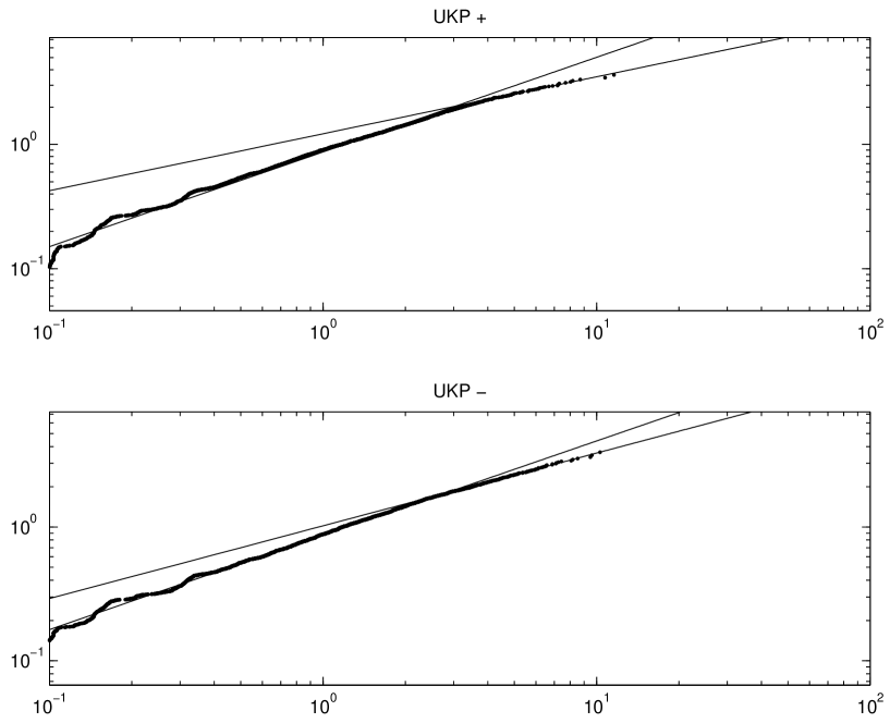
Figure 9: Graph of Gaussianized British Pound returns versus British Pound returns, for the time interval from Jan. 1971 to Oct. 1998. The upper graph gives the positive tail and the lower one the negative tail. The two straight lines represent the curves $y=\sqrt{2}\left(\frac{x}{\langle\chi_{\pm}\rangle}\right)^{\langle c_{\pm}\rangle}$ and $y=\sqrt{2}\left(\frac{x}{\chi_{\pm}}\right)^{c_{\pm}}$

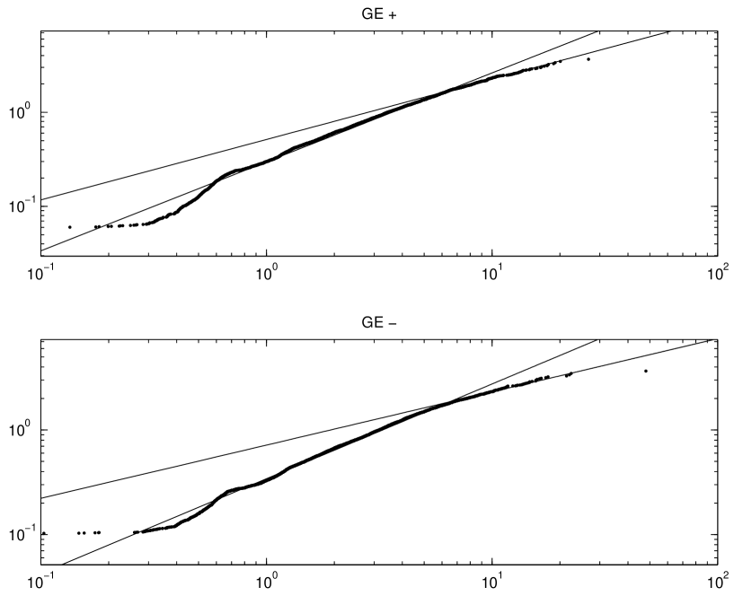
Figure 10: Graph of Gaussianized General Electric returns versus General Electric returns, for the time interval from Jan. 1970 to Dec. 2000. The upper graph gives the positive tail and the lower one the negative tail. The two straight lines represent the curves $y=\sqrt{2}\left(\frac{x}{\langle\chi_{\pm}\rangle}\right)^{\langle c_{\pm}\rangle}$ and $y=\sqrt{2}\left(\frac{x}{\chi_{\pm}}\right)^{c_{\pm}}$

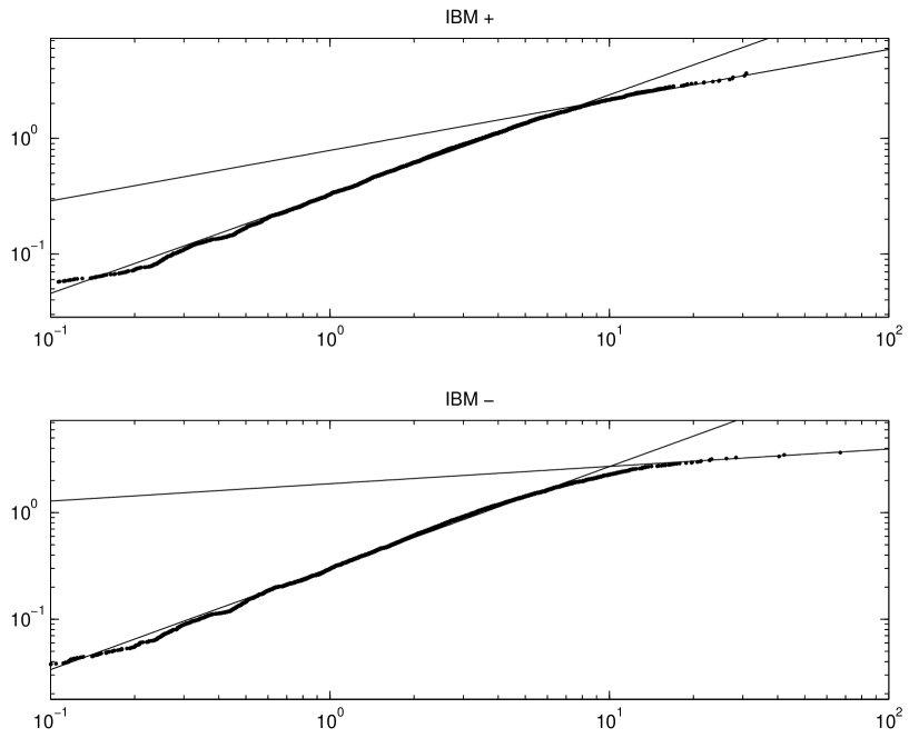
Figure 11: Graph of Gaussianized IBM returns versus IBM returns, for the time interval from Jan. 1970 to Dec. 2000. The upper graph gives the positive tail and the lower one the negative tail. The two straight lines represent the curves $y=\sqrt{2}\left(\frac{x}{\langle\chi_{\pm}\rangle}\right)^{\langle c_{\pm}\rangle}$ and $y=\sqrt{2}\left(\frac{x}{\chi_{\pm}}\right)^{c_{\pm}}$

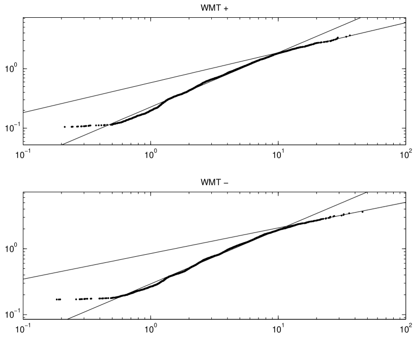
Figure 12: Graph of Gaussianized Wall Mart returns versus Wall Mart returns, for the time interval from Sep. 1972 to Dec. 2000. The upper graph gives the positive tail and the lower one the negative tail. The two straight lines represent the curves $y=\sqrt{2}\left(\frac{x}{\langle\chi_{\pm}\rangle}\right)^{\langle c_{\pm}\rangle}$ and $y=\sqrt{2}\left(\frac{x}{\chi_{\pm}}\right)^{c_{\pm}}$

References

• [1] Abramovitz, E. and I.A. Stegun, Handbook of Mathematical functions (Dover Publications, New York 1972).
• [2] Andersen, J.V., and D. Sornette, Have your cake and eat it too: increasing returns while lowering large risks! preprint at http://xxx.lanl.gov/abs/cond-mat/9907217
• [3] Artzner, P., F. Delbaen, J.M. Eber and D. Heath, Coherent measures of risk, Math. Finance 9, 203-228 (1999).
• [4] Bouchaud, J.-P., D. Sornette, C. Walter and J.-P. Aguilar, Taming large events: Optimal portfolio theory for strongly fluctuating assets, International Journal of Theoretical and Applied Finance 1, 25-41 (1998).
• [5] Embrechts, P., C. Kluppelberg and T. Mikosh, Modelling extremal events (Springel-Verlag, Applications of Mathematics 33, 1997).
• [6] Embrecht, P., A. McNeil and D. Straumann, Correlation and Dependence in risk management: properties and pitfalls, Proceedings of the Risk Management workshop, October 3, 1998 at the Newton Institute Cambridge, Cambridge University Press.
• [7] Frisch, U. and D.Sornette, Extreme Deviations and Applications, J. Phys. I France 7, 1155-1171 (1997).
• [8] Gopikrishnan, P., M. Meyer, L.A. Nunes Amaral and H.E. Stanley, Inverse cubic law for the distribution of stock price variations, European Physical Journal B 3, 139-140 (1998).
• [9] Gradshteyn, I.S. and I. M. Ryzhik, Table of integrals Series and Products, Academic Press, 1965.
• [10] Hill, B.M., A Simple General Approach to Inference about the Tail of a Distribution, Annals of statistics, 3(5), 1163-1174 (1975).
• [11] Jorion, P., Value-at-Risk: The New Benchmark for Controlling Derivatives Risk (Irwin Publishing, Chicago, IL, 1997).
• [12] Karlen, D., Using projection and correlation to approximate probability distributions, Computer in Physics 12, 380-384 (1998).
• [13] Laherrère, J. and D. Sornette, Stretched exponential distributions in nature and economy : ”fat tails” with characteristic scales, European Physical Journal B 2, 525-539 (1998).
• [14] Lindskog, F., Modelling Dependence with Copulas,
$http://www.risklab.ch/Papers.html\#MTLindskog$
• [15] Litterman, R. and K. Winkelmann, Estimating covariance matrices (Risk Management Series, Goldman Sachs, 1998).
• [16] Lux, T., The stable Paretian hypothesis and the frequency of large returns: an examination of major German stocks, Applied Financial Economics 6, 463-475 (1996).
• [17] Markovitz, H., Portfolio selection : Efficient diversification of investments (John Wiley and Sons, New York, 1959).
• [18] Merton, R.C., Continuous-time finance, (Blackwell, Cambridge, 1990).
• [19] Muzy, J.-F., D. Sornette, J. Delour and A. Arneodo, Multifractal returns and Hierarchical Portfolio Theory, Quantitative Finance 1 (1), 131-148 (2001).
• [20] Nelsen, R.B. An Introduction to Copulas. Lectures Notes in statistic, 139, Springer Verlag, New York (1998).
• [21] Pickhands, J., Statistical Inference Using Extreme Order Statitstics, Annals of Statistics, 3(1), 119-131 (1975).
• [22] Rao, C.R., Linear statistical inference and its applications, 2d ed. (New York Willey, 1973).
• [23] Sornette, D., Large deviations and portfolio optimization, Physica A 256, 251-283, 1998.
• [24] Sornette, D., Critical Phenomena in Natural Sciences, Chaos, Fractals, Self-organization and Disorder: Concepts and Tools, 432 pp., 87 figs., 4 tabs (Springer Series in Synergetics, August 2000) ISBN 3-540-67462-4
• [25] Sornette, D., J. V. Andersen and P. Simonetti, Portfolio Theory for “Fat Tails”, International Journal of Theoretical and Applied Finance 3 (3), 523-535 (2000)
• [26] Sornette, D., P. Simonetti, J.V. Andersen, $\phi^{q}$-field theory for portfolio optimization : ”fat-tails” and non-linear correlations, Physics Reports 335 (2), 19-92 (2000).
• [27] Tsallis, C. Possible generalization of Boltzmann-Gibbs statistics, J. Stat. Phys. 52, 479-487 (1988); for updated bibliography on this subject, see $http://tsallis.cat.cbpf.br/biblio.htm$.