Fermi surface renormalization in Hubbard ladders

Abstract

We derive the one-loop renormalization equations for the shift in the Fermi-wavevectors for one-dimensional interacting models with four Fermi-points (two left and two right movers) and two Fermi velocities $v_{1}$ and $v_{2}$. We find the shift to be proportional to $(v_{1}-v_{2})U^{2}$, where $U$ is the Hubbard-$U$. Our results apply to the Hubbard ladder and to the $t_{1}-t_{2}$ Hubbard model. The Fermi-sea with fewer particles tends to empty. The stability of a saddle point due to shifts of the Fermi-energy and the shift of the Fermi-wavevector at the Mott-Hubbard transition are discussed.

PACS numbers: 75.30.Gw, 75.10.Jm, 78.30.-j

Introduction - Fermi-surface properties of one- and two- dimensional interacting electron systems are a fascinating topic of current interest, motivated in part by the opening of a pseudogap in underdoped cuprates. Several novel effects have been found in generalized renormalization-group (RG) approaches to weak coupling models, in particular the formation of quasiparticle gaps [1] and a Pomaranchuk [2] and charge [3] instability in $N$-patch 2D-Hubbard models [4, 5].

Novel Fermi-surface effects are possible also in N-band 1D-dimensional interacting models, e.g. N-leg ladders [6]. Interest in the field of ladders systems has grown rapidly in the last years due to the discovery of superconductiviy in a doped two-leg ladder material [7, 8] and due to the fact that a rigorous weak-coupling analysis can be carried through.

There have been a number of previous RG investigations of 1D interacting two-band systems. Penc and Sólyom [9] extended an earlier calculation of Varma and Zawadowski [10] and studied the Fermi-velocity renormalization at two-loop. Fabrizio [11] considered the role of the transverse hopping $t_{p}$ on the stability of the Luttinger-liquid (LL) state both for the case of particles with and without spin. Balents and Fisher [12] considered the same model we do, a general 1D model with four Fermi points. There are several phases with $x$ gapless charge and $y$ gapless spin modes (notation: C$x$S$y$) in the phase diagram wich were identified by Balents and Fisher considering the bosonized form of the leading divergent running couplings. The new feature we wish to stress is that the general phase diagram is influenzed by the RG-flow of the Fermi vectors, which we evaluate explicitly. This Fermi-surface effect is especially strong near a saddle point.

It is well known [13] that the tadpole (or Harttree) diagram contributes to the renormalization of the quadratic part of the original Hamiltonian, thus leading to a renormalization of the chemical potential in the case of a one-band model. Alternatively, one might wish to work with a constant density of particles. This can be achieved by the introduction of appropriate counter terms to the chemical potential [13]. Here we would like to point out, that the tadpole diagram leads, in general, to different quadratic terms, which we denote by $\mu_{1}$ and $\mu_{2}$, for the two bands in a 1D two-band model, see Fig. 1. The renormalization of the chemical potential is given in the 2-band case by suitable avarage of $\mu_{1}$ and $\mu_{2}$. The difference of the two quadratic terms results, on the other hand, in a renormalization of the interchain hopping $t_{p}$ and thus alters the band structure.

RG-equations - We will consider for a start a general two-band model with a linearized one-particle spectrum around the Fermi-points $k_{1}$ and $k_{2}$ and denote with $v_{1}$ and $v_{2}$ the Fermi-velocities for the first band ($L_{1}$ and $R_{1}$) and second band ($L_{2}$ and $R_{2}$) respectively. Lateron we will specify our results to the case of the Hubbard ladder and $t_{1}-t_{2}$ Hubbard model. Since we will be working at one-loop, we will keep the Fermi-velocities constant throughout the calculation, even when the Fermi-points $k_{1}$ and $k_{2}$ are allowed to shift.

A list of possible coupling constants is given in Table I. The special couplings $g_{2v}$, $g_{w}$, $g_{1v}$ and $g_{s}$ exist only for the $t_{1}-t_{2}$ Hubbard model. The couplings listed come in two flavors, namely for scattering between parallel and antiparallel spins ($||$ and $\perp$) for backward scattering, $g_{\gamma 1j}$, and forward scattering, $g_{\gamma 2j}$, with $\gamma=1,2,x,t$ and $j=\parallel,\perp$. Back- and forward scattering amplitudes for parallel spins are not independent, we choose $g_{\gamma 1\parallel}\equiv 0$.

Spin-rotational invariance implies that the RG-flow leaves the combinations

$$g_{\gamma\rho}:=-{g_{\gamma 2\parallel}+g_{\gamma 2\perp}\over 2}~{},\qquad g_{\gamma\sigma}:=2g_{\gamma 1\perp}$$ (1)

invariant ($\gamma=1,2,x,t$), Here the index $\rho$ and $\sigma$ denote the charge and spin component respectively.

TABLE I.: Coupling constants for (a) Umklapp and (b) normal scattering processes ($k_{2}>k_{1}$ has been assumed). For the $t_{1}-t_{2}$ Hubbard model one has to interchange $R_{2}\leftrightarrow L_{2}$, compare Fig. (1) and (3).

label	condition	process(a)	label	process(b)
$g_{2u}$	$k_{2}=\pi/2$	$L_{2}L_{2}\to R_{2}R_{2}$	$g_{2}$	$L_{2}R_{2}\to L_{2}R_{2}$
$g_{2v}$	$3k_{2}+k_{1}=2\pi$	$L_{2}L_{2}\to R_{1}R_{2}$	$g_{1}$	$L_{1}R_{1}\to L_{1}R_{1}$
$g_{w}$	$3k_{2}-k_{1}=2\pi$	$L_{2}L_{2}\to L_{1}R_{2}$	$g_{x}$	$L_{1}R_{2}\to L_{1}R_{2}$
$g_{xu}$	$k_{2}+k_{1}=\pi$	$L_{2}L_{2}\to R_{1}R_{1}$	$g_{t}$	$L_{2}R_{2}\to L_{1}R_{1}$
$g_{tu}$	$k_{2}+k_{1}=\pi$	$L_{2}L_{1}\to R_{1}R_{2}$	$g_{s}$	$L_{2}R_{1}\to L_{1}L_{1}$
$g_{1v}$	$k_{2}+3k_{1}=2\pi$	$L_{2}L_{1}\to R_{1}R_{1}$		($3k_{1}=k_{2}$)
$g_{1u}$	$k_{1}=\pi/2$	$R_{1}R_{1}\to L_{1}L_{1}$

The RG-equations to one-loop and momentum cut-off $\Lambda$ are for general densities[12]

$\displaystyle\begin{array}[]{rlrl}\dot{g}_{1\rho}=&\beta\left(g_{t\rho}^{2}+\frac{3}{16}g_{t\sigma}^{2}\right)&\dot{g}_{1\sigma}=&-\alpha g_{1\sigma}^{2}-\frac{\beta g_{t\sigma}^{2}}{2}+2\beta g_{t\rho}g_{t\sigma}\\ \dot{g}_{2\rho}=&\alpha\left(g_{t\rho}^{2}+\frac{3}{16}g_{t\sigma}^{2}\right)&\dot{g}_{2\sigma}=&-\beta g_{2\sigma}^{2}-\frac{\alpha g_{t\sigma}^{2}}{2}+2\alpha g_{t\rho}g_{t\sigma}\\ \dot{g}_{x\rho}=&-\left(g_{t\rho}^{2}+\frac{3}{16}g_{t\sigma}^{2}\right)&\dot{g}_{x\sigma}=&-g_{x\sigma}^{2}-\frac{1}{2}g_{t\sigma}^{2}-2g_{t\rho}g_{t\sigma}\\ \dot{g}_{t\rho}=&g_{0\rho}g_{t\rho}+\frac{3g_{0\sigma}g_{t\sigma}}{16}&\dot{g}_{t\sigma}=&g_{0\sigma}g_{t\rho}\,+\\ &&&\left(g_{0\rho}-{g_{0\sigma}\over 2}-2g_{x\sigma}\right)g_{t\sigma}~{},\end{array}$

where the coupling constants have been rescaled by $1/(\pi(v_{1}+v_{2}))$, $t=-\ln(\Lambda/\Lambda_{0})$ ($\Lambda_{0}$ is the initial cut-off) and where we have introduced

$$\alpha\ =\ {v_{1}+v_{2}\over 2\,v_{1}}~{},\qquad\beta\ =\ {v_{1}+v_{2}\over 2\,v_{2}}$$ (2)

($1/\alpha+1/\beta=1$). The initial values of the rescaled coupling constants are

$$g_{\gamma\rho}\ =\ {-U\over 2\pi(v_{1}+v_{2})}~{},\qquad g_{\gamma\sigma}\ =\ {2U\over\pi(v_{1}+v_{2})}$$ (3)

for the Hubbard model. Inclusion of Umklapp scattering at special fillings leads to additional terms. They are

$$\begin{array}[]{rcl}\dot{g}_{1\rho}&=&\dots\,-\,\alpha g_{1u}^{2}\\ \dot{g}_{1u}&=&-\,4\alpha\,g_{1u}g_{1\rho}\end{array}$$ (4)

for $g_{1u}$, where the dots in the first equation denote the generic terms[14]. We find

$$\begin{array}[]{rcl}\dot{g}_{t\rho}&=&\dots\,+\,{\alpha\over 2}g_{s}^{2}~{},\qquad\dot{g}_{t\sigma}\ =\ \dots\,-\,2\alpha\,g_{s}^{2}\\ \dot{g}_{s}&=&g_{s}\,\Big{(}\,-2\alpha g_{1\rho}-3g{x\sigma}/4+g_{x\rho}\,\Big{)}\end{array}$$ (5)

for $g_{s}$ and

$$\begin{array}[]{rcl}\dot{g}_{\gamma^{\prime}\rho}&=&\dots\,-\,\alpha g_{1v}^{2}~{},\qquad\dot{g}_{1\rho}\ =\ \dots\,-\,2g_{1v}^{2}\\ \dot{g}_{1v}&=&g_{1v}\,\Big{(}\,-2g_{t\rho}-2g{x\rho}-2\alpha g_{1\rho}\,\Big{)}\end{array}$$ (6)

for $g_{1v}$ (with $\gamma^{\prime}=x,t$). The RG-equations can be solved numerically, we present in Fig. 2 a typical flow diagram for some selected coupling constants.

Phase diagram - Above RG-equations can be easily implemented either for the Hubbard ladder or for the $t_{1}-t_{2}$ Hubbard with respective dispersion relations

$$\begin{array}[]{rcl}E_{\pm}^{(lad)}(k)&=&\pm t_{p}-2t\cos(k)\\ E^{(12)}(k)&=&-2t_{1}\cos(k)-2t_{2}\cos(2k)~{}.\end{array}$$ (7)

The reflection symmetry in the Hubbard ladder (exchange of the two legs) forbids any coupling with an odd number of operators per band, see Tables I and II.

In Fig. 3 we present the phase-diagram for the $t_{1}-t_{2}$ Hubbard model, for which the control-parameter $\beta$ takes the form

$$\beta\ =\ {v_{1}+v_{2}\over 2v_{2}}\ =\ {\sin(k_{1})+\sin(k_{2})\over 2\sin(k_{2})}~{},$$ (8)

At half filling $k_{2}-k_{1}=\pi/2$. Depending on $\beta$, various coupling constants might scale to strong coupling, the divergence is in general of the form $\sim g^{*}/(t^{*}-t)$. In Table II a complete list of the diverging coupling constants is given. The differences between the Hubbard ladder and the $t_{1}-t_{2}$ Hubbard model, which stem from the different geometries of the two Fermi-seas, are pointed out in Table II.

The Umklapp scattering $g_{2u}$ at $k_{2}=\pi/2$ is not active in the $t_{1}-t_{2}$ Hubbard model, since $k_{2}>\pi/2$ for this model. $g_{2v}$ is allowed in the $t_{1}-t_{2}$ Hubbard model and would leads to a C1S0 phase if (a) $3k_{2}+k_{1}=2\pi$ and (b) $\beta>2.4$. It turns out, that it is not possible to satisfy both conditions at the same time. Inspecting the fix-point Hamiltonian and bosonizing the diverging coupling constants [12], see Table II, one finds that the number of gapless charge and spin modes are C1S2 (1u,2u), C1S0 (1v,2v), C1S1 (s,w) and C0S0 (xu,tu).

RG of Fermi-wavevectors - The renormalization equations for the local chemical potentials are given by the tadpole diagram:

$$\dot{\mu}_{i}\ =\ \Lambda(v_{1}+v_{2})\left(g_{i\rho}+g_{x\rho}\right)~{},\qquad(i=1,2)~{}.$$ (9)

Note that the cut-off $\Lambda$ occurs on the right-hand side of Eq. (9) and that the $\dot{\mu}_{i}$ are linear in the coupling constants. Let’s consider now a renormalization step, we write

$$\Delta\mu_{i}\ =\ \Delta\mu_{i}^{0}\,+\,\Delta\mu_{ct}~{},$$ (10)

where the counter-term $\Delta\mu_{ct}$ is introduced in order to enforce particle number conservation.

TABLE II.: Diverging coupling constants in all possible phases, $\kappa=\mbox{max}(\alpha,\beta)$.

phase	conditions	divergent couplings
		$\to(-\infty)$	$\to(+\infty)$
C2S2	$\kappa>4.8$	(none)	(none)
C2S1	$4.8>\beta>4.3$	$g_{1\sigma}$	(none)
C2S1	$4.8>\alpha>4.3$	$g_{2\sigma}$	(none)
C1S0	$4.3>\kappa$	$g_{t\rho},g_{x\rho},g_{1,2\sigma}$	$g_{t\sigma},g_{1,2\rho},(g_{x\sigma})^{\ddagger}$
1u		$g_{1\rho}$	$g_{1u}$
2u†		$g_{2\rho}$	$g_{2u}$
1v∗,2v∗†	$\kappa>2.4$	$g_{t\rho},g_{x\rho},g_{1,2\sigma}$	$g_{t\sigma},g_{1,2\rho},g_{x\sigma}$
s∗		$g_{x\rho},g_{1\rho},g_{t\rho}$	$g_{s},g_{2\rho}$
w∗		$g_{x\rho},g_{2\rho},g_{t\rho}$	$g_{w},g_{1\rho}$
xu†,tu†		$g_{tu\rho}$	$g_{xu},g_{tu\sigma}$
		$g_{t\rho},g_{x\rho},g_{1,2\sigma}$	$g_{t\sigma},g_{1,2\rho},g_{x\sigma}$

^∗Does not occur in the ladder due to transversal momentum conservation.
^† Does not occur in the $t_{1}-t_{2}$ model due to conditions on $k_{1}$ and $k_{2}$.
^‡ Subleading divergence $\sim g_{x\sigma}^{*}/\sqrt{t^{*}-t}$.

The counter term is compensated by subtracting the corresponding term from the interaction part of the Hamiltonian. The size of $\Delta\mu_{ct}$ is determined for the Hubbard ladder by the condition ($\Delta k_{i}v_{i}=\Delta\mu_{i}^{0}$)

$$\Delta k_{1}\ =\ -\Delta k_{2}~{},\qquad v_{2}\Delta\mu_{1}^{0}\ =\ -v_{1}\Delta\mu_{2}^{0}$$ (11)

(for the $t_{1}-t_{2}$ Hubbard model $\Delta k_{1}=\Delta k_{2}$ etc.), which leads to

$$\begin{array}[]{rcl}\displaystyle\Delta\mu_{i}^{0}&=&(-1)^{i}\,{v_{i}\over v_{1}+v_{2}}\big{(}\Delta\mu_{2}-\Delta\mu_{2}\big{)}\\ \displaystyle\Delta\mu_{ct}&=&{v_{1}\over v_{1}+v_{2}}\Delta\mu_{2}+{v_{2}\over v_{1}+v_{2}}\Delta\mu_{1}~{}.\end{array}$$ (12)

Eq. (12) and Eq. (9) lead then to

$$\dot{k}_{i}\ =\ (-1)^{i}\Lambda\left(g_{2\rho}-g_{1\rho}\right)~{},$$ (13)

which describes the flow of the Fermi-wavevector. Since the initial values for $g_{1\rho}$ and $g_{2\rho}$ are identical, see Eq. (3), a non-trivial renormalization of the Fermi-wavevector occurs only when $v_{1}\neq v_{2}$, i.e. when $\alpha\neq\beta$. For the Luttinger-liquid phase C2S2 the limit

$$\Delta k_{i}=\lim_{t\to\infty}\int_{0}^{t}dt^{\prime}\,\dot{k}_{i}(t^{\prime})$$ (14)

is well defined. In the other phases there is normally a plateau in $\Delta k_{i}(t)=\int_{0}^{t}dt^{\prime}\,\dot{k}_{i}(t^{\prime})$, due to the decreasing cut-off $\Lambda$ in the expression (13) for $\dot{k}_{i}$ which can be considered to define an approximate $\Delta k_{i}$, see Fig. 2.

Let us consider the flow of the Fermi-wavevector in some more detail for the Hubbard ladder, where $k_{1}<k_{2}$ and $v_{1}<v_{2}$. The relation $\alpha>\beta$ then leads generally to $g_{2\rho}>g_{1\rho}$ and consequently to

$$\Delta k_{1}\ <\ 0~{},\qquad\Delta k_{2}\ >\ 0~{}.$$ (15)

The smaller Fermi-sea tends to empty.

In the limit $U\to 0$ the renormalization of the coupling constants tends to zero in the C2S2 phase, and one can obtain an asymptotic rigorous expression for the total shift $\Delta k=-\Delta k_{1}$ using ($i=1,2$)

$\displaystyle g_{i\rho}(t)\ \approx\ g_{i\rho}(0)+\dot{g}_{i\rho}(0)\,t~{},\qquad\dot{g}_{i\rho}(0)\ =\ {U^{2}/2\over v_{1}+v_{2}}{1\over\pi^{2}v_{3-i}}$

and Eq. (3) for $g_{i\rho}(0)$. With (13) and (14) we obtain

$$\Delta k \approx {\Lambda_{0}U^{2}/2\over\pi^{2}(v_{1}+v_{2})}\left({1\over v_{1}}-{1\over v_{2}}\right)$$ (16)

$$= {U^{2}\over\pi^{2}}\,{\alpha-\beta\over(v_{1}+v_{2})^{2}}\,\Lambda_{0}~{}.$$ (17)

The Fermi-surface renormalization effects become especially strong near a saddle point, where $v_{1}\ll v_{2}$, i.e. $\alpha\gg\beta$. Eq. (17) has been derived for the case of the Hubbard ladder. For the $t_{1}-t_{2}$ Hubbard model one has just to interchange $\alpha\leftrightarrow\beta$, both Fermi-points shift then in the same direction (to larger values), see the inset of Fig. 3.

Discussion - In above discussion of the Fermi-surface renormalization we have kept the Fermi-velocities $v_{1}$ and $v_{2}$. At two-loop, the Fermi-velocities are renormalized, an effect $O(U^{3})$. The change of $\delta k$ is, on the other hand, quadratic in $U$ and leads therefore (for the ladder) to an additional reduction in $v_{1}$, which is $O(U^{2})$. This reduction in $v_{1}/v_{2}$ would lead to a further enhancement of $\Delta k$ in a self-consistent treatment. We do not, however, expand this point here further, since it would involve a somewhat uncontrolled mixture of high- and low-energy scales.

It is of interest, however, to study the stability of the saddlepoint itself. This question has been studied extensively for the case of $N$-patch models of the 2D Hubbard model. Honerkamp et al. [1] have found, that particles tend to leave the saddle-point region (also called ‘hot spots’), in accordance to our result Eq. (17). Gonzalez et al. [3, 15] have found that the saddle point attracts the Fermi-level both from above and from below.

We have therefore considered the case when the Fermi-level is exactly at the bottom of the first band in the Hubbard ladder. In this case the usual RG-approach has to be modified. We have followed the approach proposed by Balents and Fisher [12] (an expansion in the curvature) and find with $v_{1}=0$

$$\dot{\mu}_{1}\ =\ \Lambda v_{2}g_{x\rho}\qquad\dot{\mu}_{2}=\Lambda v_{2}g_{2\rho}~{}.$$ (18)

As the initial values of $g_{x\rho}$ and $g_{2\rho}$ are identical for the Hubbard model, see Eq. (3), one has to consider the flow of $g_{x\rho}$ and $g_{2\rho}$, which is, due to the lack of scale-invariance, explicitly cut-off dependent. One finds [16] $g_{2\rho}>g_{x\rho}$, i.e. the Fermi-level is pushed below the bottom of the first band. The saddle point is therefore pushed above the Fermi-level by the RG-flow.

Mott-Hubbard transition - A Mott-Hubbard transition occurs in the half-filled one-dimensional $t_{1}-t_{2}$ model as a function of interaction strength $U$. For $t_{2}>t_{1}/2$, that is for the case of four Fermi-points, this transition occurs at finite values of $U$. Aebischer et al. estimated [17] a critical $U_{c}\sim 2.67t_{1}$ for $t_{2}=0.7t_{1}$. The question we would like to ask now is: How large is the Fermi-surface shift $\Delta k$ for $U=U_{c}$? We cannot answer this question within our weak-coupling approach, but we can estimate the order of magnitude of $\Delta k$ by assuming formula Eq. (17) to hold up to the Mott-Hubbard transition. We obtain

$$\Delta k\big{|}_{U=2.67t_{1}}^{t_{2}=0.7t_{1}}\ \approx\ 0.4\,\Lambda_{0}\ =\ 0.4\,(\pi-k_{2})~{},$$ (19)

where we have taken $\pi-k_{2}$ as a physical relevant initial cut-off. This estimate indicates that the Fermi-wavevector is shifted by a substantial fraction towards the Brillouin zone edge near the Mott-Hubbard transition. We note that the real $\Delta k$ might be even larger since we have neglected in this estimate the renormalization of the Fermi-velocity which, as we have discussed further above, would enhance the effect. In principle it would be possible that the Mott-Hubbard transition coincides with $k_{2}\to\pi$ for $U\to U_{c}$. Physically this would correspond to an activation of the one-band Umklapp scattering $g_{1u}$ at the transition point.

Conclusions - We have derived and discussed the RG-equations for the Fermi-wavevectors in one-dimensional models with four Fermi-points. We find that the renormalization of the Fermi-wavevectors is quadratic in the interaction, suggesting substantial effects at strong coupling and near the Mott-Hubbard transition. We have pointed out, that the renormalization of the Fermi-wavevector is of especial importance near a saddle point, and that it leads to changes, $\Delta v_{i}$, in the Fermi-velocities quadratic in the coupling constant $U$, whereas the usual two-loop contributions to $\Delta v_{i}$ are cubic in $U$.

In addition we have discussed the phase diagram of the 1D $t_{1}-t_{2}$ Hubbard model and found a new phase (C1S1,s/w).

Acknowledgments - This work was partially supported by the DFG. One of us (C.G.) would like to thank W. Metzner for valuable discussions.

(a)

(b)

FIG. 1.: Dispersion relation of a Hubbard ladder with interchain hopping $t_{p}$. The renormalization flow will lead, in general, to different “chemical potentials” for the two bands (a), which in turn will lead to renormalized Fermi-wavevectors (b). For the case of the Hubbard ladder, this process can be recast in a renormalization of the interladder hopping $t_{p}$.

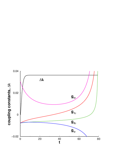
FIG. 2.: Example of the RG-flow of some selected coupling constants for the half-filled $t_{1}-t_{2}$ Hubbard model with $U=0.1t_{1}$, $t_{2}=0.7t_{1}$, $\alpha=0.63$, $\beta=2.4$ (C1S0 phase, see Fig. 3, corresponding to $k_{1}=0.418\pi$, $k_{2}=0.918\pi$ and $v_{1}=1.66t_{1}$, $v_{2}=0.43t_{1}$. The initial values of the coupling constants are given by Eq. (3). Also shown is the flow of the Fermi-surface shift $\Delta k$ (in units of $\Lambda_{0}/100$).

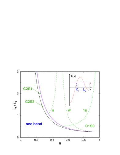
FIG. 3.: Phase diagram for the $t_{1}-t_{2}$ Hubbard model. The region denoted ‘one band’ is the C1S1 LL-phase with one band empty, $n=0.5$ denotes half-filling. Note that the ‘1u’ phase-line is continuous[14]. Inset: An illustration of the dispersion relation.

REFERENCES

- [1] N. Furukawa, T.M. Rice and M. Salmhofer, Phys. Rev. Lett. 81, 3195 (1998); C. Honerkamp, M. Salmhofer, N. Furukawa and T.M. Rice Phys. Rev. B 63, 035 109 (2001).
- [2] C.J. Halboth and W. Metzner, Phys. Rev. Lett. 85, 5162 (2000).
- [3] J. González, Phys. Rev. B 63, 45114 (2001).
- [4] J.V. Alvarez, J. Gonzalez, F. Guinea and M.A.H. Vozmediano, J. Phys. Soc. Jpn 67, 1868 (1998).
- [5] J. Gonzalez, F. Guinea, M.A.H. Vozmediano, Phys. Rev. Lett. 84, 4930 (2000).
- [6] U. Ledermann, K. Le Hur and T.M. Rice, Phys. Rev. B. 62, 16 383 (2000).
- [7] M. Uehara, T. Nagata, J. Akimitsu, H. Takahashi, N. Mori and K. Kinoshita, J. Phys. Soc. Jpn. 65, 2764 (1996).
- [8] T.M. Rice, S. Gopalan and M. Sigrist, Europhys. Lett. 23, 445 (1993).
- [9] K. Penc and J. Sólyom, Phys. Rev. B 41, 704 (1990).
- [10] C.M. Varma and A. Zawadowski, Phys. Rev. B 32, 7399 (1985).
- [11] M. Fabrizio, Phys. Rev. B 48, 15 838 (1993).
- [12] L. Balents and M.P.A. Fisher, Phys. Rev. B 53, 12 133 (1996).
- [13] R. Shankar, Rev. Mod. Phys. 66, 129 (1994).
- [14] Note the factor two difference of Eq. (4) with respect to the corresponding Eq. (3.1) in Ref. [12], which we believe to be erroneous. As a consequence of this difference the line of existence for the “1u” phase (and for the corresponding “2u” phase) are not broken in Fig. 3.
- [15] J. Gonzalez, F. Guinea and M.A.H. Vozmediano, Nucl. Phys. B 485, 694 (1997);
- [16] In [12] at the saddle point, see Eq. (3.7) of Ref. [12].
- [17] C. Aebischer, D. Baeriswyl and R.M. Noack, Phys. Rev. Lett. 86, 468 (2001).
(a)
(b)