Quantum Effects in Coulomb Blockade

Abstract

We review the quantum interference effects in a system of interacting electrons confined to a quantum dot. The review starts with a description of an isolated quantum dot. We discuss the Random Matrix theory (RMT) of the one-electron states in the dot, present the universal form of the interaction Hamiltonian compatible with the RMT, and derive the leading corrections to the universal interaction Hamiltonian. Next, we discuss a theoretical description of a dot connected to leads via point contacts. Having established the theoretical framework to describe such an open system, we discuss its transport and thermodynamic properties. We review the evolution of the transport properties with the increase of the contact conductances from small values to values $\sim e^{2}/\pi\hbar$. In the discussion of transport, the emphasis is put on mesoscopic fluctuations and the Kondo effect in the conductance.

PACS numbers: 73.23.Hk, 73.23.-b, 72.10.Bg

1 Introduction

Conventionally, electric transport in bulk materials is characterized by the conductivity $\sigma$. Then, the conductance $G$ of a finite-size sample of dimensions $L_{x}\times L_{y}\times L_{z}$ can be found by combining the conductances of its smaller parts, $G=\sigma L_{y}L_{z}/L_{x}$. This description, however, is applicable only at sufficiently high temperatures, at which the conductivity can be treated as a local quantity. It was discovered about two decades ago [1, 2] that the quantum corrections to the conductivity are non-local on the scale of the (temperature dependent) dephasing length $L_{\varphi}$, which is much larger than the elastic mean free path. If the sample is small, or the temperature low, so that $L_{\varphi}$ exceeds the sample size, the concept of conductivity loses its meaning. Moreover, the conductance $G$ acquires significant sample-to-sample fluctuations and can no longer be treated as a self-averaging quantity. For a temperature $T$ below the Thouless energy $E_{T}=\hbar/\tau_{D}$, these sample-to-sample fluctuations are of the order of the conductance quantum $e^{2}/2\pi\hbar$, independent of sample size or mean free path ($\tau_{D}$ is the time it takes for an electron to diffuse through the system). This phenomenon is called “Universal Conductance Fluctuations” (UCF), and it was studied in great detail both theoretically and experimentally, see [3, 4, 5, 6, 7] for a review. It is important to emphasize that the lack of self-averaging of the conductance is a feature of mesoscopic samples, i.e., samples with linear dimensions smaller than $L_{\varphi}$ but still much larger than the Fermi wave length.

These ideas that defined the field of mesoscopic physics were initially developed in the context of transport through disordered metals. A convenient way of creating more controllable mesoscopic samples was developed with the use of semiconductor heterostructures, see [8] for a review. As the electron motion in these systems is quantized in the direction perpendicular to the plane of the heterostructure, a two-dimensional electron gas is formed at the interface between the layers. With the help of additional electrostatic confinement, usually in the form of metal gates deposited on top of the hetrostructure, the two-dimensional electron gas (2DEG) can be tailored to form a finite-size sample, referred to as a quantum dot. Its size, shape, and connection with the rest of the 2DEG can be controlled by means of a sophisticated system of electrostatic gates, see Fig. 1.

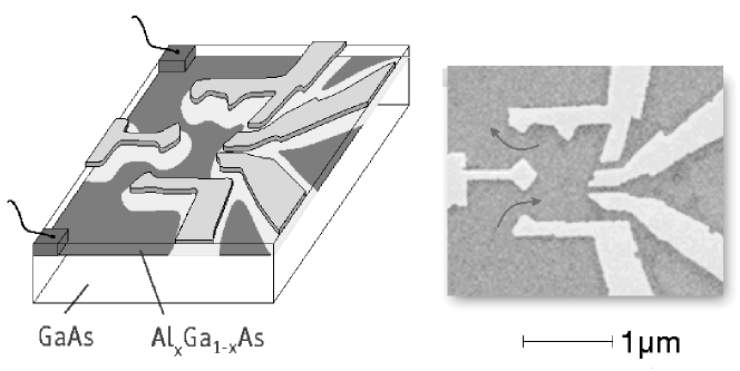
Figure 1: Micrograph of the quantum dot [9]. By changing the voltages on the gates conductances of point contacts and the shape of the dot can be changed.

Links connecting the quantum dot to the 2DEG (quantum point contacts) are characterized by the number $N_{\rm ch}$ of electron modes (or channels) propagating through the contact at the Fermi level, and by the set of transmission probabilities for these modes. With the increase of the point contact cross-section, the number of modes, $N_{\rm ch}$, is increasing. If the boundaries of the point contact are smooth on the length scale set by the electron wavelength, then the contact acts as an electron wave guide [10]: all the propagating modes, except the one which opened last, do not experience any appreciable backscattering. For the last mode, the transmission coefficient varies from $0$ to $1$ in the crossover from the evanescent to propagating behavior [5]. In the specific case of a gate-controlled contact, see Fig. 1, the distance between the gate and the depleted edge of the 2DEG is typically large compared to the electron wavelength in the electron gas [12]. The curvature radius of the edge of the 2DEG at the contact is of the order of this distance, and therefore the smoothness condition is satisfied.

A statistical ensemble of quantum dots can be obtained by slightly varying the shape of the quantum dot, the Fermi energy, or the magnetic field, keeping the properties of its contacts to the outside world fixed. Statistical properties of the conductance for such an ensemble depend on the number of modes, $N_{\rm ch}$, in the junctions and their transparency. The “usual” UCF theory adequately describes the conductance through a disordered or chaotic dot in the limit of large number of modes, $N_{\rm ch}\gg 1$. When all channels in the two point contacts are transparent, the universal value of the root mean square (r.m.s.) conductance fluctuations $\langle\delta G^{2}\rangle^{1/2}\simeq e^{2}/2\pi\hbar$ is much smaller than the average conductance $\langle G\rangle\simeq N_{\rm ch}e^{2}/2\pi\hbar$. The distribution of conductances is essentially Gaussian, and can be found theoretically by means of the standard diagrammatic expansion for disordered systems [13], or with Random Matrix Theory (RMT), see Refs. [14] and [15] for reviews. Upon closing the point contacts (i.e., decreasing $N_{\rm ch}$), the average conductance decreases whereas the r.m.s. fluctuations retains its universal value. At $N_{\rm ch}\simeq 1$, the fluctuations and the average of the conductance are of the same order, and the conductance distribution function is no longer Gaussian. Still, if one neglects the interaction between the electrons, the statistics of the conductance can be readily obtained within RMT [14, 16, 17].

The RMT of transport through quantum dots can be easily justified for non-interacting electrons. However, real electrons are charged, and thus interact with each other. It is known from the theory of bulk disordered systems, that the electron-electron interaction results in corrections to the conductance [18] of the order of unit conductance quantum $e^{2}/2\pi\hbar$. For a quantum dot connected to a 2DEG by single-mode junctions, this correction is not small anymore in comparison to the average conductance $\langle G\rangle$.

We see that at $\langle G\rangle\simeq e^{2}/2\pi\hbar$ and low temperatures, both mesoscopic fluctuations and interaction effects become strong. Quantum interference and interaction effects can not be separated, and there is no obvious expansion parameter to use for building a theory describing the statistics of the conductance in this regime. This paper reviews the current understanding of physical phenomena in a wide class of mesoscopic systems – quantum dots – under the conditions in which effects of electron-electron interaction are strong.

A first step to approach this problem is to disregard the mesoscopic fluctuations altogether. It means that one neglects the random spatial structure of the wave functions in the dot and the randomness of the energy spectrum; the discrete energy spectrum with spacing $\Delta$ between the one-electron levels in a closed dot is replaced by a continuous spectrum with the corresponding macroscopic density of states. For realistic systems, this approach can be justified sometimes at not-so-low temperatures. The remaining problem of accounting for the Coulomb interaction is non-perturbative at small conductance $G\>{{}^{{}_{\displaystyle<}}_{\displaystyle\sim}}\>e^{2}/2\pi\hbar$, and therefore still not trivial. It constitutes the essence of the so-called Coulomb blockade phenomenon [19, 8].

The Coulomb blockade manifests itself most profoundly (see, e.g., Ref. [20, 8]) in oscillations of the dot’s conductance $G(V_{g})$ with the variation of the voltage $V_{g}$ on a gate, which is capacitively coupled to the dot, see Fig. 2. The resulting dependence $G(V_{g})$ exhibits equidistant Coulomb blockade peaks separated by deep minima (Coulomb blockade valleys). The peaks occur at the charge degeneracy points, i.e., specific values of $V_{g}$ at which changing the dot charge by a single quantum $e$ does not cost any energy. The idea of the Coulomb blockade was suggested in the early experimental paper [22] in the late 1960’s, though the term “Coulomb blockade” was coined only two decades later [23]. A quantitative theory in terms of rate equations describing the transport through a blockaded quantum dot or metal grain at $G\ll e^{2}/2\pi\hbar$, was formulated in Ref. [24, 25], and was generalized to systems with a controllable gate in Ref. [23]. This theory is commonly referred to as the “orthodox theory”. The main conclusion of the orthodox theory is that the conductance through a blockaded grain at low temperatures is exponentially suppressed. The first experiments on gated metallic Coulomb blockade systems were reported in Ref. [26].

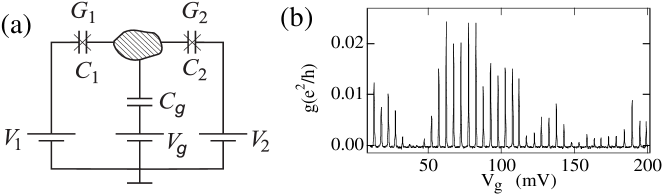
Figure 2: (a): Schematic view of the dot with the gate electrode; (b): conductance of the dot as a function of the gate voltage (from Ref. [21]).

At larger values of the dot’s conductance (corresponding to larger values of the conductances $G_{1}$ and $G_{2}$ of the point contacts connecting the dot to the outside world), the orthodox theory and, eventually, the phenomenon of Coulomb blockade break down because of quantum fluctuations of the charge in the dot. The fluctuations destroy the Coulomb blockade at the value $G\sim e^{2}/\pi\hbar$. Quantum fluctuations affect both transport properties (such as linear conductance and $I$-$V$ characteristics) and thermodynamics (e.g., differential capacitance). The $I$-$V$ characteristic in the Coulomb blockade valleys at relatively small conductance was considered in [27] in second order perturbation theory in $G$; later the corresponding non-linear contribution to the current found in [27] became known as “inelastic co-tunneling” [28]. Corrections induced by charge fluctuations at $G\ll e^{2}/\pi\hbar$ were calculated in [29] for the thermodynamic characteristics, and in [30, 31, 40, 32] for the linear conductance. At $G\ll e^{2}/\pi\hbar$ the problem of quantum charge fluctuations was mapped [33] on the multi-channel Kondo problem [34, 35], which in some cases can be solved exactly [36, 37].

Another limit which allows for a comprehensive solution, is the case of a point contact with one almost open conducting channel linking the dot to the lead (conductance $G$ is close to the conductance quantum) [38, 39, 40]. In this limit, and still neglecting mesoscopic fluctuations ($\Delta=0$), the Coulomb blockade almost vanishes: the contribution periodic in the gate voltage $V_{g}$ to the differential capacitance, which is the prime signature of Coulomb blockade, is small compared to the average capacitance [39]. Moreover, it was shown within this model that the Coulomb blockade disappears completely in the case where the channel is fully transparent.

In all of the aforementioned works the effects of mesoscopic fluctuations, associated with the finite size and the discrete energy spectrum of the isolated dot (nonzero level spacing $\Delta$), were ignored. However, these fluctuations drastically affect the results. In open dots, mesoscopic fluctuations reinstate periodic oscillations of the differential capacitance and conductance as a function of the gate voltage $V_{g}$, as a remnant the charge discreteness in the dot, even in the limit of completely transparent channels in the point contacts. If the dot is almost closed, the chaotic nature of the wave functions in the dot gives rise to mesoscopic fluctuations of observable quantities. Both in the Coulomb blockade valleys and at the peaks, the conductance turns out to have large fluctuations, and is very sensitive to a magnetic field.

Our main goal in this paper is to review the rich variety of effects associated with the finite level spacing $\Delta$, the chaotic nature of the wave functions, and the Coulomb interaction for both closed and open dots. Here is a one-paragraph guide to the review. Sections 2, 3, and 4 are devoted, respectively, to the physics of an isolated quantum dot, transport through a dot weakly connected to leads, and thermodynamic and transport properties of a dot connected to lead(s) by one or two almost reflectionless quantum point contacts. We begin in Section 2 with the formulation of the model describing the statistical properties of the system. We clarify the conditions of the equivalence of the usual diagrammatic technique and Random Matrix representation, and establish the validity of the capacitive interaction approximation. The central result of this part can be found in Subsection 2.3.3, where we present the universal form of the interaction Hamiltonian describing the dot, and estimate the accuracy of the universal description. In Section 3 we review the theory of mesoscopic fluctuations of the conductance in peaks and valleys of the Coulomb blockade, and the theory of the Kondo effect in quantum dots. Weak dot-lead coupling allows us to use the familiar technique of the perturbation theory in tunneling strength. We believe it makes Section 3 easy to read. Nevertheless, a very pragmatic reader who wants to grasp the main results first, without going through the details, may start by reading the summary in Subsection 3.4. Section 4 deals with the similar phenomena in quantum dots connected to leads by transparent or almost transparent point contacts, where the interplay between quantum charge fluctuations and mesoscopic physics becomes especially interesting. Methods described and used in Section 4 are technically more involved than in Section 3, and include the bosonization technique along with the effective action formalism. To make the navigation through the material easier, we decided to start this Section with a presentation of the main results for the conductance through a dot and for its thermodynamics, see Subsection 4.1. Along with providing the general picture for the conductance and differential capacitance, this Subsection points to formulas valid in various important limiting cases, which are derived later in Subsections 4.6–4.7. Subsections 4.2–4.4 review the main physical ideas built into the theory, while the details of the rigorous theory are presented in Subsection 4.5. Last but not least, we illustrate the application of theoretical results by briefly reviewing the existing experimental material, see Subsections 3.1–3.3, and 4.8.

2 The model

In Subsections 2.1 and 2.2 we discuss the electronic properties of an isolated quantum dot. Under the assumption that electron motion inside the dot is chaotic, we establish a hierarchy of energy scales for the free-electron spectrum: Fermi energy, Thouless energy, and level spacing. The correlation between electronic eigenstates and eigenvalues can be described by Random Matrix Theory (RMT) if the difference between the corresponding energy eigenvalues is smaller than the Thouless energy. In subsection 2.3 we proceed with the inclusion of effects of the interaction between the electrons. It is shown that the two-particle interaction matrix elements also have hierarchical structure. The largest matrix elements correspond to charging of the quantum dot, as described by the charging energy in the constant interaction model. Finally, open quantum dots are discussed in Subsection 2.4, where we introduce the Hamiltonian of the junctions connecting the dot with the leads and relate the parameters of this Hamiltonian to the characteristics of the quantum point contacts.

2.1 Non-interacting electrons in an isolated dot: Status of RMT

Let us start from a picture of non-interacting electrons, postponing the introduction of electron-electron interactions to Sec. 2.3. The dot is described by the Hamiltonian

$$\hat{H}_{F}=\int d\vec{r}\left[\frac{1}{2m}\vec{\nabla}\hat{\psi}^{\dagger}\vec{\nabla}\hat{\psi}+U\left(\vec{r}\right)\hat{\psi}^{\dagger}\hat{\psi}\right],$$ (1)

where the electron creation (annihilation) operators obey canonical anticommutation relations

$$\left\{\hat{\psi}\left(\vec{r}_{1}\right),\hat{\psi}\left(\vec{r}_{2}\right)\right\}=0,\ \ \left\{\hat{\psi}^{\dagger}\left(\vec{r}_{1}\right),\hat{\psi}\left(\vec{r}_{2}\right)\right\}=\delta\left(\vec{r}_{1}-\vec{r}_{2}\right).$$ (2)

The potential $U(\vec{r})$ describes the confinement of electrons to the dot, as well as the random potential (if any) inside the dot. We will neglect the spin-orbit interaction; The one-particle Hamiltonian then is diagonal in spin space, and for the time being we omit the spin indices.

The eigenfunctions of the Hamiltonian (1) are Slater determinants built from single-particle states with wavefunctions defined by the Schroedinger equation

$$\left[-\frac{\vec{\nabla}^{2}}{2m}+U\left(\vec{r}\right)\right]\phi_{\alpha}\left(\vec{r}\right)=\varepsilon_{\alpha}\phi_{\alpha}\left(\vec{r}\right).$$ (3)

In this orthonormal basis

$$\hat{H}_{F}=\sum_{\alpha}\varepsilon_{\alpha}\hat{\psi}^{\dagger}_{\alpha}\hat{\psi}_{\alpha},$$ (4)

where the fermionic operators $\hat{\psi}_{\alpha}$ are defined as $\hat{\psi}_{\alpha}\equiv\int d\vec{r}\hat{\psi}\left(\vec{r}\right)\phi_{\alpha}^{*}\left(\vec{r}\right)$ and have the usual anticommutation relations, cf. Eq. (2).

Each particular eigenstate depends sensitively on the details of the random potential $U(\vec{r})$, which is determined by the shape of the quantum dot. However, we will not be interested in the precise value of observables that depend on the detailed realization of the potential $U(\vec{r})$. Instead, our goal is a statistical description of the various response functions of the system with respect to external parameters such as magnetic field, gate voltage, etc., and of the correlations between the response functions at different values of those parameters. Hereto, the statistical properties of a response function are first related to the correlation function of the eigenstates of the Hamiltonian (3). Then, we can employ the known results for statistics of the eigenvalues and eigenvectors in a disordered or a chaotic system [41, 42, 43, 44].

For a disordered dot, the correlation functions are found by an average of the proper quantities over the realizations of the random potential. Such averaging can be done by means of the standard diagrammatic technique for the electron Green functions

$${\cal G}^{R,A}(\varepsilon,\vec{r}_{1},\vec{r}_{2})=\sum_{\alpha}\frac{\phi_{\alpha}^{*}(\vec{r}_{2})\phi_{\alpha}(\vec{r}_{1})}{\varepsilon-\varepsilon_{\alpha}\pm i0},$$ (5)

where plus and minus signs correspond to the retarded (R) and advanced (A) Green functions respectively.

The spectrum of one-electron energies is fully characterized by the density of states

$$\nu(\varepsilon)=\sum_{\alpha}\delta\left(\varepsilon-\varepsilon_{\alpha}\right)=\frac{1}{2\pi i}\int d\vec{r}\left[{\cal G}^{A}(\varepsilon,\vec{r},\vec{r})-{\cal G}^{R}(\varepsilon,\vec{r},\vec{r})\right],$$ (6)

where the last equality follows immediately from the definition (5). Even though the density of states is a strongly oscillating function of energy, its average is smooth,

$$\langle\nu(\varepsilon)\rangle=\frac{1}{\Delta(\varepsilon)},$$ (7)

where ${\Delta(\varepsilon)}$ is the mean one-electron level spacing. It varies on the characteristic scale of the order of the Fermi energy $E_{F}$, measured, say, from the conduction band edge, which is the largest energy scale in the problem. Since we are interested in quantities associated with a much smaller energy scale, we can neglect the energy dependence of the mean level spacing. The average in Eq. (7), denoted by brackets $\langle\dots\rangle$, is performed over the different realizations of the random potential for the case of a disordered dot, or over an energy strip of width $\gg\Delta$, but $\ll E_{F}$ for a clean (i.e., ballistic) system.

The average density of states does not carry any information about the correlations between the energies of different eigenstates. Such information is contained in the correlation functions for the electron energy spectrum. Probably, the most important example is the two-point correlation function ${\cal R}^{(2)}(\omega)$,

$${\cal R}^{(2)}(\omega)=\Delta^{2}\langle\nu(\varepsilon)\nu(\varepsilon+\omega)\rangle-1.$$ (8)

To calculate ${\cal R}^{(2)}(\omega)$, one substitutes the expression (6) for the density of states in terms of the Green functions $G^{R}$ and $G^{A}$ into Eq. (8),

$${\cal R}^{(2)}(\omega)=\frac{\Delta^{2}}{2\pi^{2}}{\mathrm{R}e}\int d\vec{r}_{1}d\vec{r}_{2}\langle{\cal G}^{R}\left(\varepsilon+\omega,\vec{r}_{1},\vec{r}_{1}\right){\cal G}^{A}\left(\varepsilon,\vec{r}_{2},\vec{r}_{2}\right)\rangle-1.$$ (9)

When the dot contains many electrons — which is the case of interest here — the size of the dot and the region of integration in Eq. (9) greatly exceed the Fermi wavelength. In that case, averaging of the products ${\cal G}^{R}{\cal G}^{A}$ using the diagrammatic technique yields two contributions to the integrand in (9), proportional to the squares of diffuson and Cooperon propagators in coinciding points, respectively, see Fig. 3. The result of such a calculation [41],

$${\cal R}^{(2)}(\omega)=\frac{\Delta^{2}}{\beta\pi^{2}}\mbox{Re}\,\sum_{\gamma_{n}}\frac{1}{\left(i\omega+\gamma_{n}\right)^{2}},$$ (10)

is expressed in terms of the eigenvalues $\gamma_{n}$ of the classical diffusion operator,

$$-D\vec{\nabla}^{2}f_{n}(\vec{r})=\gamma_{n}f_{n}(\vec{r}),$$ (11)

supplemented by von Neumann boundary conditions at the boundary of the dot. Here $D$ is the electron diffusion coefficient in the dot, and the Dyson symmetry parameter $\beta=1$ ($2$) in the presence (absence) of time reversal symmetry. Ensembles of random systems possessing and not possessing this symmetry are called Orthogonal and Unitary ensembles, respectively. Being derived by means of diagrammatic perturbation theory, Eq. (10) and Eq. (12) below are valid for energy differences $\omega\gg\Delta$ only. The exact results, valid for all $\omega$, are also available, see, e.g., Refs. [43, 44, 45, 46, 47]; however, the approximation (10) is sufficient for the present discussion. An expression similar to Eq. (10) is believed to be valid for a chaotic and ballistic quantum dot. The only difference with the diffusive case is that instead of the eigenvalues of the diffusion operator one has to use eigenvalues $\gamma_{n}$ of a more general (Perron-Frobenius) operator of the classical relaxational dynamics [49]; in this case the eigenvalues $\gamma_{n}$ can be complex with ${\mathrm{R}e}\,\gamma_{n}>0$, see also Appendix A.

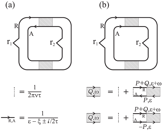
Figure 3: Diagrammatic expansion of the correlation of the density of states for the disordered system [41]. In the presence of magnetic field (unitary ensemble, $\beta=2$) the Cooperon diagram (b) is suppressed. In the figure, the symbols $P$ and $Q$ refer to the momenta of the electrons; $P$ is the large momentum, $|P-k_{F}|\ll k_{F}$, $Q$ is the small momentum $|Q|\ll k_{F}$; $\xi=P^{2}/2m-\mu$, where $\mu$ is the chemical potential; in two dimensions, the mean free time $\tau$ is related to the diffusion constant $D$ through $D=v_{F}^{2}\tau/2$, $v_{F}$ being the Fermi velocity.

The relation of ${\cal R}^{(2)}(\omega)$ to the dynamics of a particle in a closed volume allows one to draw an important conclusion regarding the universality of ${\cal R}^{(2)}(\omega)$. Note that a spatially uniform particle density satisfies the relaxational dynamics or the diffusion equation. Because of particle number conservation, such a solution is time independent. Therefore, the lowest eigenvalue $\gamma_{0}$ in Eq. (11) must be zero, independent of the shape of the dot and the strength of the disorder,

$${\cal R}^{(2)}(\omega)=-\frac{\Delta^{2}}{\beta\pi^{2}\omega^{2}}+\frac{\Delta^{2}}{\beta\pi^{2}}{\mathrm{R}e}\sum_{\gamma_{n}\neq 0}\frac{1}{\left(i\omega+\gamma_{n}\right)^{2}}\quad.$$ (12)

The first term in Eq. (12) is universal. One can immediately see that if $\hbar\omega$ is much smaller than the Thouless energy $E_{T}\equiv\hbar{\mathrm{R}e}\,\gamma_{1}$, the remaining terms in Eq. (12) are small compared to the first one and can be neglected.

The universal part of the correlation function (12) can be reproduced within a model where the Hamiltonian (1) is replaced by a hermitian matrix with random entries

$$\hat{H}_{F}=\sum_{\alpha,\gamma}{\cal H}_{\alpha\gamma}\hat{\psi}^{\dagger}_{\alpha}\hat{\psi}_{\gamma}\quad.$$ (13)

The coefficients ${\cal H}_{\alpha\gamma}$ in Eq. (13) form a real ($\beta=1$) or complex ($\beta=2$) random Hermitian matrix ${{\cal H}}$ of size $M\times M$, belonging to the Gaussian ensemble

$$\langle{\cal H}_{\alpha\gamma}{\cal H}_{\alpha^{\prime}\gamma^{\prime}}\rangle=\frac{M\Delta^{2}}{\pi^{2}}\left[\delta_{\alpha\gamma^{\prime}}\delta_{\alpha^{\prime}\gamma}+\left(2/\beta-1\right)\delta_{\alpha\alpha^{\prime}}\delta_{\gamma\gamma^{\prime}}\right],\quad\beta=1,2.$$ (14)

The Hamiltonian (13), with the distribution of matrix elements (14) reproduces the universal part of the spectral statistics of the microscopic Hamiltonian (1) in the limit $M\to\infty$ of large matrix size. The condition $\Delta\ll E_{T}$, provides the significant region $\omega\ll E_{T}$ where the non-universal part of the two level correlator ${\cal R}_{2}(\omega)$ could be neglected. and where the replacement of the microscopic Hamiltonian by the matrix model (13), is meaningful. This condition may be reformulated as the requirement that the dimensionless conductance $g$ of the dot be large, where

$$g\equiv\frac{\hbar\gamma_{1}}{\Delta}=\frac{E_{T}}{\Delta}\gg 1.$$ (15)

A large value of $g$ indicates that the dot can be treated as a good conductor.

We now present explicit expressions for the dimensionless conductance $g$ for a disc-shaped dot for two simple models: (i) a dot of radius $R$ exceeding the electron mean free path $l$, and (ii) a ballistic dot of radius $R$ with a boundary which scatters electrons diffusively, see Ref. [51, 52] and references therein.

For a diffusive dot, one needs to solve Eq. (11) to obtain $\gamma_{1}=Dx_{1}/R^{2}$, where $x_{1}\approx 2.40$ is the first zero [53] of the Bessel function, $J_{0}(x_{1})=0$. Using the electron density of states in two-dimensional electron gas, one finds $\Delta=2\hbar^{2}/mR^{2}$, and the conductance is

$$g=\frac{x_{1}}{4}k_{F}l=\frac{2\pi\hbar}{e^{2}}\frac{x_{1}}{4\pi R_{\Box}}.$$

Here $k_{F}$ is the Fermi wave vector, and $R_{\Box}$ is the resistance per square of the two-dimensional electron gas. Note that $g$ is independent of the radius of the dot in the case of the diffusive electron motion.

For the model (ii), the eigenvalue ${\mathrm{R}e}\,\gamma_{1}\approx 0.38v_{F}/R$ of the Liouville operator with the diffusive boundary conditions was found in Ref. [51], and one finds

$$g=0.19k_{F}R.$$

2.2 Effect of a weak magnetic field on statistics of one-electron states in the dot

Physical properties of a mesoscopic system are manifestly random. The statistics of the random behavior can be studied by a measurement of the fluctuations caused by the application of an external magnetic field $B$. The role of such a field is primarily to alter the quantum interference pattern. As a result, the characteristic fields which significantly affect the properties of a mesoscopic system are rather weak in a classical sense: the cyclotron radius of an electron remains much larger than the linear size of the dot, and the effect of the magnetic fields on classical trajectories can be neglected.

A magnetic field can be included in the random matrix model of Eq. (13). In order to include the magnetic field, we have to take the matrix ${\cal H}_{mn}$ in Eq. (13) from a crossover ensemble that interpolates between the orthogonal ($\beta=1$) and unitary ($\beta=2$) ensembles [54, 55, 56]:

$${\cal H}_{\alpha\gamma}=\left(1+X^{2}\right)^{-1/2}\left({\cal H}_{\alpha\gamma}^{s}+iX{\cal H}_{\alpha\gamma}^{a}\right).$$ (16)

Here ${\cal H}_{mn}^{s(a)}$ is the random realization of independent Gaussian real symmetric (antisymmetric) $M\times M$ matrices,

$$\langle{\cal H}_{\alpha\gamma}^{a(s)}{\cal H}_{\alpha^{\prime}\gamma^{\prime}}^{a(s)}\rangle=\frac{M\Delta^{2}}{\pi^{2}}\left[\delta_{\alpha\alpha^{\prime}}\delta_{\gamma\gamma^{\prime}}\pm\delta_{\alpha\gamma^{\prime}}\delta_{\alpha^{\prime}\gamma}\right],$$ (17)

where “$+$” (“$-$”) sign corresponds to the symmetric (antysimmetric) part of the Hamiltonian. In Eq. (16), $X$ is a real parameter proportional to the magnetic field (the precise relation between $X$ and $B$ is given below), so that the time reversal symmetry is preserved,

$${\cal H}_{\alpha\gamma}(B)={\cal H}_{\gamma\alpha}(-B).$$ (18)

The prefactor $(1+X^{2})^{-1/2}$ in Eq. (16) is chosen in such a way that the mean level spacing $\Delta$ remains unaffected by the magnetic field.

The correlation function of elements of the Hamiltonian (16) at different values of the magnetic field $B_{1,2}$ can be conveniently written similarly to Eq. (14) as

$$\langle{\cal H}_{\alpha\gamma}(B_{1}){\cal H}_{\alpha^{\prime}\gamma^{\prime}}(B_{2})\rangle = \frac{M\Delta^{2}}{\pi^{2}}$$

$$\mbox{}\times\left[\delta_{\alpha\gamma^{\prime}}\delta_{\alpha^{\prime}\gamma}\left(1-\frac{N_{h}^{D}}{4M}\right)+\delta_{\alpha\gamma}\delta_{\alpha^{\prime}\gamma^{\prime}}\left(1-\frac{N_{h}^{C}}{4M}\right)\right].$$

The dimensionless quantities $N_{h}^{D,C}$, which characterize the effect of the magnetic field on the wave-functions and the spectrum of the closed dot, are related to the original parameters $X$ as

$$N_{h}^{D}=2M\left(X_{1}-X_{2}\right)^{2},\ \ N_{h}^{C}=2M\left(X_{1}+X_{2}\right)^{2},$$

where the normalization is chosen in a way that the size of the matrix $M$ does not enter into physical quantities in the physically relevant limit $M\gg 1$.

The relationship between the parameter $X$ and the real magnetic field applied to the dot is best expressed with the help of $N_{h}^{D}$ and $N_{h}^{C}$,

$$N_{h}^{D}=\chi g\left(\frac{\Phi_{1}-\Phi_{2}}{\Phi_{0}}\right)^{2},\quad N_{h}^{C}=\chi g\left(\frac{\Phi_{1}+\Phi_{2}}{\Phi_{0}}\right)^{2},$$ (20)

where $g\gg 1$ is the dimensionless conductance of the closed dot, see Eq. (15), $\Phi_{1(2)}$ is the magnetic flux through the dot at the magnetic field $B_{1(2)}$, $\Phi_{0}=hc/e$ is the flux quantum, and $\chi$ is a geometry dependent numerical factor of order unity. A derivation of Eq. (20) is sketched at the end of this subsection. We also refer the reader to Refs. [57, 58]. Here we give the values of the constant $\chi$ for two specific cases: (i) $\chi=\pi/x_{1}\approx 1.31$ for a disk-shaped diffusive dot, and (ii) $\chi\approx 2.78$ for a disc-shaped ballistic dot with diffusive boundary scattering [52].

The random matrix description (16)—(2.2) is valid provided $N_{h}^{D,C}\ll g$. At larger values of the magnetic field, a universal description is no longer applicable. However, for most physical quantities, the crossover between the orthogonal and unitary ensembles takes place at $N_{h}^{D,C}\simeq 1$, i.e., well within the regime where the RMT description is appropriate.

A small magnetic field significantly affects the correlations of the eigenvectors and eigenvalues of the random Hamiltonian (16). For the pure orthogonal and unitary ensembles ($\beta=1$ and $2$, respectively), the eigenvectors and eigenvalues are independent of each other. Moreover, in the limit $M\to\infty$, the eigenvectors of different eigenstates are independently distributed Gaussian variables,

$$\langle\psi_{\alpha}(i)\psi_{\gamma}^{\ast}(j)\rangle=\frac{\delta_{ij}\delta_{\alpha\gamma}}{M},\quad\langle\psi_{\alpha}(i)\psi_{\gamma}(j)\rangle=\left(\frac{2}{\beta}-1\right)\frac{\delta_{ij}\delta_{\alpha\gamma}}{M}.$$ (21)

In other words, an eigenvector can be represented as

$$\psi_{\alpha}(n)=\frac{1}{\sqrt{M}}\frac{\left(u_{n}+it_{\alpha}v_{n}\right)}{\sqrt{1+t_{\alpha}^{2}}}$$ (22)

where $M$ is the size of the matrix, $u,v$ are independent real Gaussian variables, $\langle u_{n}u_{m}\rangle=\delta_{nm}$, $\langle v_{n}v_{m}\rangle=\delta_{nm}$, $\langle u_{n}v_{m}\rangle=0$, and $t_{\alpha}=0$ ($1$) for the orthogonal (unitary) ensemble [59, 54]. Equation (22) is a consequence of the symmetry of the distribution of the random matrices with respect to an arbitrary rotation of the basis. At the crossover between those two ensembles, this symmetry no longer exists, which leads to a departure of the distribution of $\psi_{\alpha}(n)$ from a (real or complex) Gaussian [60, 61], and to correlations of the values of the wave functions at different sites [62, 63]. It was noticed in Refs. [64, 65] that the crossover between the orthogonal and unitary ensembles can be described by using the decomposition (22) where the parameter $t_{\alpha}$ is no longer fixed at the extremal values $t=0$ or $t=1$, but a fluctuating quantity $0\leq t\leq 1$ with the distribution function [60, 61, 62, 63]

$$W(t) = \left(\frac{\pi N_{h}^{C}}{8}\right)\left(\frac{1-t^{4}}{t^{3}}\right)\exp\left[-\left(\frac{\pi N_{h}^{C}}{16}\right)\left(\frac{1-t^{2}}{t}\right)^{2}\right]$$

$$\times \left\{\phi\left(\frac{\pi N_{h}^{C}}{4}\right)+\left[\left(\frac{1+t^{2}}{2t}\right)^{2}-\frac{4}{\pi N_{h}^{C}}\right]\left[1-\phi\left(\frac{\pi N_{h}^{C}}{4}\right)\right]\right\},$$

$$\phi(x) = \int_{0}^{1}dy\exp\left[-x\left(1-y^{2}\right)\right],$$ (23)

where $N_{h}^{C}$ is given by Eq. (20) with $\Phi_{1}=\Phi_{2}\equiv\Phi$, being the magnetic flux through the dot. We see, that the crossover between two ensembles occurs at characteristic scale of the magnetic field $N_{h}^{C}\simeq 1$, or using (20), at $\Phi=\Phi_{0}/(2\sqrt{\chi g})$. Equation (23) completely describes the distribution of a single eigenvector. In order to find the statistics of the quantities contributed by several levels, it is necessary to find the joint distribution of $t_{\alpha}$ of several levels, $W(t_{1},t_{2},\dots)$. The exact form of such a distribution function is not known.

In the opposite limiting case when a physical result is contributed to by a large number of levels, it is possible to use the conventional diagrammatic technique [13] to calculate different moments of the Green functions

$${\cal G}^{R,A}_{ij}(\varepsilon)=\sum_{\alpha}\frac{\psi_{\alpha}(i)\psi_{\alpha}^{\ast}(j)}{\varepsilon-\varepsilon_{\alpha}\pm i0},$$ (24)

see also Eq. (5). The diagrammatic calculation shown in Fig. 4 yields

$$\left\langle{\cal G}^{R}_{jk}(\varepsilon+\omega,B_{1}){\cal G}^{A}_{lm}(\varepsilon,B_{2})\right\rangle=\frac{2\pi}{M^{2}\Delta}\left(\frac{\delta_{jm}\delta_{kl}}{-i\omega+N_{h}^{D}\frac{\Delta}{2\pi}}+\frac{\delta_{jl}\delta_{km}}{-i\omega+N_{h}^{C}\frac{\Delta}{2\pi}}\right),$$

(25)

where $N_{h}^{C}$ and $N_{h}^{D}$ are defined in Eq. (2.2). The irreducible averages $\langle{\cal G}^{A}{\cal G}^{A}\rangle$ or $\langle{\cal G}^{R}{\cal G}^{R}\rangle$ are smaller than Eq. (25) by factor of $\omega/(M\Delta)$ and can be disregarded in the thermodynamic limit $M\to\infty$. All the higher moments can be expressed in terms of the second moments (25) with the help of the Wick theorem.

Equation (25) can serve as a starting point to relate the quantities $N_{h}^{D}$, $N_{h}^{C}$ to the real magnetic field, thus providing a derivation of Eq. (20). To establish such a relation, one needs to recalculate the average (25) using the microscopic Hamiltonian (1). The result is again given by Eq. (10), where now the magnetic field is introduced into the diffusion equation of Eq. (11) by the replacement of $\partial/\partial{\vec{r}}$ by the covariant derivative $\partial/\partial{\vec{r}}+i(e/c\hbar){\vec{A}^{\pm}}({\vec{r}})$, and a modification of the boundary condition to ensure that the particle flux through the boundary remains zero. The vector-potentials ${\vec{A}^{\pm}}({\vec{r}})$ are related to the magnetic fields ${\vec{B}}_{1}$ and ${\vec{B}}_{2}$ by $\mbox{curl}\,{\vec{A}^{\pm}}={\vec{B}}_{1}\pm{\vec{B}}_{2}$. The corresponding lowest eigenvalues $\gamma_{0}^{-}$ and $\gamma_{0}^{+}$ are identified with $(\Delta/2\pi)N_{h}^{D}$ and $(\Delta/2\pi)N_{h}^{C}$ respectively. A similar replacement can be also made in the Liouville equation for the ballistic system.

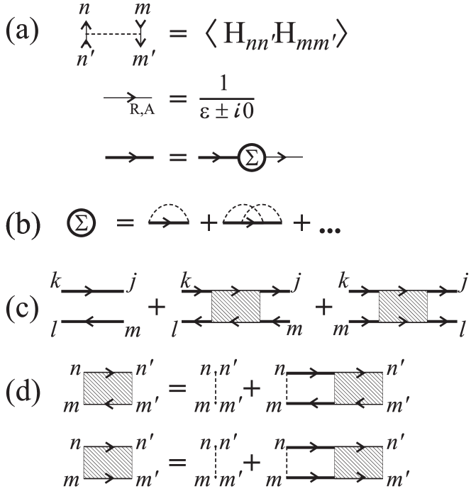
Figure 4: (a) analytic expressions for the lines on the diagrams; (b) diagrams for self-energy $\hat{\Sigma}$. The second term in the self-energy includes an intersection of the dashed lines ant it is smaller than the first term by a factor $1/M$. (c), (d) diagrammatic representation for irreducible averages (25).

We close this subsection with a more elaborate discussion of Eq. (25) and its physical interpretation. Hereto, we consider the case of equal magnetic fields $B_{1}$ and $B_{2}$, i.e., $N_{h}^{D}=0$. Then, one sees from Eq. (25) that a weak magnetic field introduces new energy scale

$$\hbar/\tau_{h}^{C}=\Delta N^{C}_{h}/2\pi$$ (26)

If this scale is smaller than the Thouless energy $E_{T}$, the universal description holds, and we find that the system under consideration is at the crossover between the Orthogonal and Unitary ensembles. Phenomena associated with the energy scale smaller than $\hbar/\tau_{h}^{C}$, are described effectively by the unitary ensemble, whereas phenomena associated with larger energy scales still can be approximately described by the orthogonal ensemble. This conclusion allows for a simple semiclassical interpretation of the relation (20) between $N_{h}^{C}$ and the real magnetic field $B$, as we now explain.

Consider a classical trajectory of an electron starting from a point ${\bf r}$ and returning to the same point, see Fig. 5. The quantum mechanical amplitude for this process contains an oscillating term $e^{i{\cal S}_{\rm cl}/\hbar}$, where ${\cal S}_{\rm cl}$ is the classical action along this trajectory. In a weak magnetic field the classical trajectory does not change, while the classical action acquires an Aharonov - Bohm phase:

$${\cal S}_{\rm cl}\to{\cal S}_{\rm cl}+\frac{eB}{c}{\cal A}_{\rm cl},$$ (27)

where ${\cal A}_{\rm cl}$ is the directed area swept by the trajectory, see Fig. 5. If the time it takes for the electron to return along the trajectory, $t$, would be of the order of the ergodic time $\hbar/E_{T}$, the characteristic value of this area would be of the order of the geometrical area of the dot $|{\cal A}_{\rm cl}|\simeq{\cal A}_{\rm dot}$ (the meaning of the Thouless energy $E_{T}$ is discussed in previous subsections). If, however, $t\gg\hbar/E_{T}$, the electron trajectory covers the dot $N_{t}\simeq tE_{T}/\hbar$ times. Each winding through the dot adds a value of the order of ${\cal A}_{\rm dot}$ to ${\cal A}_{\rm cl}$; these contributions, however, are of random signs, (an example is shown in Fig. 5). Therefore, the total area accumulated scales with $\sqrt{N_{t}}$,

$$|{\cal A}_{\rm cl}|\simeq{\cal A}_{\rm dot}\sqrt{N_{t}}\simeq{\cal A}_{\rm dot}\left(\frac{tE_{T}}{\hbar}\right)^{1/2}.$$ (28)

The orthogonal ensemble is different from the unitary ensemble by the fact that in the orthogonal ensemble the quantum mechanical amplitudes corresponding to a pair of time reversed trajectories have the same phase, while these phases are unrelated for the unitary ensemble. For a small magnetic field, this means, that the trajectories which acquired an Aharonov-Bohm phase smaller than unity still effectively belong to the orthogonal ensemble whereas, those which acquire a larger phase are described by the unitary ensemble. To obtain the characteristic time scale separating these two regimes, we require

$$\frac{eB|{\cal A}_{\rm cl}|}{c}\simeq\hbar.$$ (29)

Substituting estimate (28) into Eq. (29), and using $\Phi=B{\cal A}_{\rm dot}$, one finds

$$\frac{1}{t}\simeq\frac{E_{T}}{\hbar}\left(\frac{\Phi}{\Phi_{0}}\right)^{2}.$$ (30)

Up to a numerical coefficient, this estimate coincides with the energy scale given by Eqs. (26) and (20). The small energy scale physics is governed by long trajectories with a typical accumulated flux larger than the flux quantum. For such trajectories the interference between the time reversal paths is already destroyed. At larger energy scales, the contributing trajectories are shorter, and they do not accumulate enough magnetic field flux to destroy the interference.

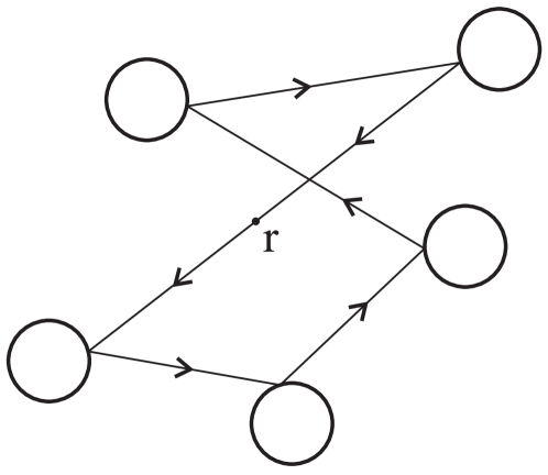
Figure 5: Example of the self-returning trajectories.

2.3 Interaction between electrons: The universal description

Let us now turn to the discussion of interaction between electrons in a quantum dot. In the basis of eigenfunctions $\phi_{\alpha}$ of the free-electron Hamiltonian, the two-particle interaction takes the form:

$$\hat{H}_{\rm int}={\textstyle\frac{1}{2}}\sum{\cal H}_{\alpha\beta\gamma\delta}\psi^{\dagger}_{\alpha,\sigma_{1}}\psi^{\dagger}_{\beta,\sigma_{2}}\psi_{\gamma,\sigma_{2}}\psi_{\delta,\sigma_{1}}.$$ (31)

Hereinafter, we will write explicitly the spin indices $\sigma$ for the fermionic operators. The generic matrix element of interaction is:

$${\cal H}_{\alpha\beta\gamma\delta}=\int d\vec{r}_{1}d\vec{r}_{2}V(\vec{r}_{1}-\vec{r}_{2})\phi_{\alpha}(\vec{r}_{1})\phi_{\beta}(\vec{r}_{2})\phi_{\gamma}^{*}(\vec{r}_{2})\phi_{\delta}^{*}(\vec{r}_{1}).$$ (32)

Our goal is to show that the matrix elements of the interaction Hamiltonian also have hierarchical structure: Only a few of these elements are large and universal, whereas the majority of them are proportional to the inverse dimensionless conductance $1/g$, and thus small  [67, 69, 66, 68, 70]. As the result, Hamiltonian (31) will be separated into two pieces:

$$\hat{H}_{\rm int}=\hat{H}_{\rm int}^{(0)}+\hat{H}_{\rm int}^{(1/g)}.$$ (33)

The first term here is universal, does not depend on the geometry of the dot, and it does not fluctuate from sample to sample for samples differing only by realizations of disorder. The second term is small as a power of $1/g$, and it fluctuates. This term only weakly affects the low-energy ($E\>{{}^{{}_{\displaystyle<}}_{\displaystyle\sim}}\>E_{T}$) properties of the system.

The form of the universal term can be established using the requirement of compatibility of this term with the Random Matrix model (13). Since the Random Matrix distribution is invariant with respect to an arbitrary rotation of the basis, the operator $\hat{H}_{\rm int}^{(0)}$ may include only operators invariant under such rotations. In the absence of the spin-orbit interaction, there are three such operators:

$$\hat{n}=\sum_{\alpha,\sigma}\hat{\psi}^{\dagger}_{\alpha,\sigma}\hat{\psi}_{\alpha,\sigma};\quad\hat{\vec{S}}={\textstyle\frac{1}{2}}\sum_{\alpha}\hat{\psi}^{\dagger}_{\alpha,\sigma_{1}}\vec{\sigma}_{\sigma_{1}\sigma_{2}}\hat{\psi}_{\alpha,\sigma_{2}};\quad\hat{T}=\sum_{\alpha}\hat{\psi}_{\alpha,\uparrow}\hat{\psi}_{\alpha,\downarrow}.$$ (34)

The operator $\hat{n}$ is the total number of particles, $\hat{\vec{S}}$ is the total spin of the dot, and operator $\hat{T}$ corresponds to the interaction in the Cooper channel. (For the unitary ensemble the operator $\hat{T}$ is not allowed.)

Gauge invariance requires that only the product $T^{\dagger}T$ of the operators ${\hat{T}}$ and ${\hat{T}}^{\dagger}$ can enter into the Hamiltonian. At the same time, $SU(2)$ symmetry dictates that the Hamiltonian may depend only on $({\hat{\vec{S}}})^{2}$, and not on separate components of the spin vector. Taking into account that the initial interaction Hamiltonian (31) is proportional to $\psi^{4}$, we find for its universal part:

$$\hat{H}_{\rm int}^{0}=E_{c}\hat{n}^{2}+J_{S}\left(\hat{\vec{S}}\right)^{2}+J_{c}\hat{T}^{\dagger}\hat{T}.$$ (35)

The three terms in the Hamiltonian (35) have a different meaning. The first two terms represent the dependence of the energy of the system on the total number of electrons and total spin, respectively. Because both total charge and spin commute with the free-electron Hamiltonian, these two terms do not have any dynamics for a closed dot. We will see that the situation will change with the opening of contacts to the leads. Finally, the third term corresponds to the interaction in the Cooper channel, and it does not commute with the free-electron Hamiltonian (1) or (13). This term is renormalized if one considers contributions in higher order perturbation theory in the interaction. For an attractive interaction, $J_{c}<0$, the renormalization enhances this interaction, eventually leading to the superconducting instability. (We will not consider the case of an attractive interaction here; for a recent review on the physics of small superconducting grains, see Ref. [71]. Effects in larger grains, $E_{c}\gg\Delta$, are reviewed in Ref. [72].) For the repulsive case, $J_{c}>0$, this term renormalizes logarithmically to zero. We will be dealing with the latter case throughout the paper.

Constants in the Hamiltonian (35) are model-dependent. In the remainder of this subsection we will show how to calculate them for some particular interactions and discuss the structure of the non-universal part ${\hat{H}}^{(1/g)}$.

At this point it is important to mention that universal Hamiltonian (35) is defined within the Hilbert space of one-electron states with energies of the order or less than Thouless energy. The matrix elements of this Hamiltonian are not just the matrix elements of the interaction potential (32). This potential is defined in a much wider energy strip which includes one-electron states with energies $\simeq E_{F}$. Virtual transitions between the low-energy ($\>{{}^{{}_{\displaystyle<}}_{\displaystyle\sim}}\>E_{T}$) sector and these high-energy states renormalize the matrix elements of the universal Hamiltonian. It turns out [13] that the third term in the Hamiltonian (35) corresponding to the Cooper channel of interaction, can be strongly renormalized by such virtual transitions. In order to avoid this complication, we will consider the case of the unitary ensemble in the discussion below, where the “bare” matrix elements corresponding to the Cooper channel are already suppressed by a weak magnetic field (it is sufficient to thread a flux of the order of unit quantum $\Phi_{0}$ through the cross-section of a dot), and relegate the corresponding discussion of the interaction in the Cooper channel to the Appendix B. Omission of the Cooper channel here is a simplification that will not affect our principal conclusions, as we will consider the case of repulsive interaction where the Cooper channel, if it were included, is renormalized to zero anyway.

The statistics of the interaction matrix elements can now be related to the properties of the one-electron wave functions. The easiest way to study the statistics of the wave-functions $\phi_{\alpha}(\vec{r})$ is to relate them to the Green functions (5) and then use the diagrammatic technique for the averaging of their products. From Eq. (5) we have

$${\cal G}^{A}(\varepsilon;\vec{r}_{1},\vec{r}_{2})-{\cal G}^{R}(\varepsilon;\vec{r}_{1},\vec{r}_{2})=2\pi i\sum_{\alpha}\phi_{\alpha}(\vec{r}_{1})\phi_{\alpha}^{*}(\vec{r}_{2})\delta(\varepsilon-\varepsilon_{\alpha}).$$ (36)

At given energy $\varepsilon$, at most one eigenstate contributes to the sum in Eq. (36). Furthermore, it is known that there is no correlation between the statistics of levels and that of wave functions in the lowest order in $1/g$, see, e.g., Ref. [41], so we can neglect the level correlations and average the $\delta$-function in Eq. (36) independently. As a result, we can estimate

$$\phi_{\alpha}(\vec{r}_{1})\phi_{\alpha}(\vec{r}_{2})^{*}\theta(\delta/2-|\varepsilon_{\alpha}-\varepsilon|)\approx\frac{1}{2\pi}\!\!\!\int_{\varepsilon-\delta/2}^{\varepsilon+\delta/2}d\varepsilon_{1}\left[{\cal G}(\varepsilon_{1};\vec{r}_{1},\vec{r}_{2})\right]_{-},\,\delta\ll\Delta,$$ (37)

where we introduced the notation

$$\left[{\cal G}(\varepsilon;\vec{r}_{1},\vec{r}_{2})\right]_{-}=-i\left[{\cal G}^{A}(\varepsilon;\vec{r}_{1},\vec{r}_{2})-{\cal G}^{R}(\varepsilon;\vec{r}_{1},\vec{r}_{2})\right].$$ (38)

Let us first calculate the average of the matrix element (32). Because of the randomness of the wave functions, the corresponding product in Eq. (32) does not vanish only if its indices are equal pairwise. It is then readily expressed with the help of Eq. (37),

$$\frac{\delta^{2}}{\Delta^{2}}\langle\phi_{\alpha}(\vec{r}_{1})\phi_{\beta}(\vec{r}_{2})\phi_{\gamma}^{*}(\vec{r}_{3})\phi_{\delta}^{*}(\vec{r}_{4})\rangle$$

$$=\frac{1}{4\pi^{2}}\int_{-\delta/2}^{\delta/2}d\varepsilon_{1}\int_{-\delta/2}^{\delta/2}d\varepsilon_{2}\left[\delta_{\alpha\delta}\delta_{\beta\gamma}\langle\left[{\cal G}(\varepsilon_{\alpha}+\varepsilon_{1};\vec{r}_{1},\vec{r}_{4})\right]_{-}\left[{\cal G}(\varepsilon_{\beta}+\varepsilon_{2};\vec{r}_{2},\vec{r}_{3})\right]_{-}\rangle\right.$$

$$\left.+\delta_{\alpha\gamma}\delta_{\beta\delta}\langle\left[{\cal G}(\varepsilon_{\alpha}+\varepsilon_{1};\vec{r}_{1},\vec{r}_{3})\right]_{-}\left[{\cal G}(\varepsilon_{\beta}+\varepsilon_{2};\vec{r}_{2},\vec{r}_{4})\right]_{-}\rangle\right]$$ (39)

In deriving Eq. (39) for $\alpha\neq\beta$ we have used the relation

$$\langle\phi_{\alpha}(\vec{r}_{1})\phi_{\alpha}(\vec{r}_{2})^{*}\phi_{\beta}(\vec{r}_{1})\phi_{\beta}(\vec{r}_{2})^{*}\theta(\delta/2-|\varepsilon_{\alpha}-\varepsilon|)\theta(\delta/2-|\varepsilon_{\beta}-\varepsilon|)\rangle$$

$$=\langle\phi_{\alpha}(\vec{r}_{1})\phi_{\alpha}(\vec{r}_{2})^{*}\phi_{\beta}(\vec{r}_{1})\phi_{\beta}(\vec{r}_{2})^{*}\rangle\langle\theta(\delta/2-|\varepsilon_{\alpha}-\varepsilon|)\theta(\delta/2-|\varepsilon_{\beta}-\varepsilon|)\rangle$$

$$=\frac{\delta^{2}}{\Delta^{2}}\langle\phi_{\alpha}(\vec{r}_{1})\phi_{\alpha}(\vec{r}_{2})^{*}\phi_{\beta}(\vec{r}_{1})\phi_{\beta}(\vec{r}_{2})^{*}\rangle.$$

The result (39) can be justified also for $\alpha=\beta$ and $k_{F}|\vec{r}_{1}-\vec{r}_{2}|\gg 1$ (with $k_{F}$ being the Fermi wavevector), see Ref. [68]. The corrections to Eq. (39) are of the order or smaller than $1/g^{2}$, and will be neglected since we are interested in the leading in $1/g$ terms.

In the leading approximation in $1/g$ needed to derive $\hat{H}^{(0)}_{\rm int}$, the Green function entering into the products in the above formula may be averaged independently. Substituting

$$\langle\left[{\cal G}(\varepsilon_{\alpha}+\varepsilon_{1};\vec{r}_{1},\vec{r}_{2})\right]_{-}\rangle=\frac{2\pi}{\Delta{\cal V}_{d}}{\cal F}\left(k_{F}|\vec{r}_{1}-\vec{r}_{2}|\right);$$ (40)

$${\cal F}\left(k_{F}|\vec{r}|\right)=\langle e^{i\vec{k}\cdot\vec{r}}\rangle_{FS},$$

with $\langle\dots\rangle_{FS}$ denoting the average over the electron momentum on the Fermi surface, into Eq. (39), we find

$${\left({\cal V}_{d}\right)^{2}}\langle\phi_{\alpha}(\vec{r}_{1})\phi_{\beta}(\vec{r}_{2})\phi_{\gamma}^{*}(\vec{r}_{3})\phi_{\delta}^{*}(\vec{r}_{4})\rangle^{(0)}=\\ \left[\delta_{\alpha\delta}\delta_{\beta\gamma}{\cal F}_{14}{\cal F}_{23}+\delta_{\alpha\gamma}\delta_{\beta\delta}{\cal F}_{13}{\cal F}_{24}\right],$$ (41)

where we introduced the short-hand notation

$${\cal F}_{ij}\equiv{\cal F}\left(k_{F}|\vec{r}_{i}-\vec{r}_{j}|\right),$$ (42)

and ${\cal V}_{d}$ is the volume of a $d$-dimensional grain. Equation (41) does not depend on the disorder strength and corresponds to the universal limit. The coordinate dependence in function ${\cal F}$ indicates simply that all the plane waves that are allowed by the conservation of energy are represented in the wave function.

2.3.1 Universal description for the case of short-range interaction

We start with the model case of a weak short range interaction

$$V(\vec{r})=\lambda\Delta{\cal V}_{d}\delta(\vec{r})$$ (43)

to illustrate the principle, and then discuss the realistic long range Coulomb interaction. In Eq. (43), ${\cal V}_{d}$ is the volume of the dot in dimension $d=3$ or its area for $d=2$, and $\lambda\ll 1$ is the interaction constant.

Averaging of the matrix elements (32) with the help of Eq. (41) allows us to derive the Hamiltonian $\hat{H}^{(0)}_{\rm int}$ from Eq. (31). Indeed, such averaging yields

$${\cal H}_{\alpha\beta\gamma\delta}^{(0)}=\lambda\Delta\left(\delta_{\alpha\delta}\delta_{\beta\gamma}+\delta_{\alpha\gamma}\delta_{\beta\delta}\right).$$ (44)

Now we substitute Eq. (44) into Eq. (31) and rearrange the summation over spin indices with the help of identity

$$2\delta_{\sigma_{1}\sigma_{2}}\delta_{\sigma_{3}\sigma_{4}}=\delta_{\sigma_{1}\sigma_{3}}\delta_{\sigma_{2}\sigma_{4}}+\vec{\sigma}_{\sigma_{1}\sigma_{3}}\vec{\sigma}_{\sigma_{4}\sigma_{2}},$$

where $\vec{\sigma}=\left(\hat{\sigma}^{x},\hat{\sigma}^{y},\hat{\sigma}^{z}\right)$ and $\hat{\sigma}^{k}$ are the Pauli matrices in the spin space. As a result, the interaction Hamiltonian takes the universal form (34), (35), with the coupling constants

$$E_{c}={\textstyle\frac{1}{4}}\lambda\Delta;\quad J_{S}=-\lambda\Delta;\quad J_{c}=0.$$ (45)

The vanishing of $J_{c}$ is a feature of the unitary ensemble, see also Appendix B. We see that for a weak short-range repulsive interacton all the matrix elements in the universal part of the Hamiltonian are smaller than the level spacing. Later we will see that for the Coulomb interaction this is not the case, and the constant $E_{c}$ is large compared with $\Delta$.

We derived the universal Hamiltonian (35) in the leading approximation, which corresponds to the limit $1/g\to 0$. In this approximation, only the “most diagonal” matrix elements of the interaction Hamiltonian are finite. In the first order in $1/g$, there are two types of the corrections $H_{\alpha\beta\gamma\delta}^{(1/g)}$ to the universal Hamiltonian. First, the matrix elements of the diagonal part of the Hamiltonian, Eq. (35), acquire a correction $\propto 1/g$. This correction exhibits mesoscopic fluctuations and has a non-zero average value. Second, the non-diagonal matrix elements of the interaction Hamiltonian for a mesoscopic quantum dot become finite, but with zero average value.

We start with the evaluation of the average correction $\langle H_{\alpha\beta\gamma\delta}^{(1/g)}\rangle$ to the matrix elements $H_{\alpha\beta\gamma\delta}^{(0)}$ of the Hamiltonian (35),

$$\langle H_{\alpha\beta\gamma\delta}^{(1/g)}\rangle=\langle{H_{\alpha\beta\gamma\delta}}\rangle-H_{\alpha\beta\gamma\delta}^{(0)}.$$ (46)

To this end, we have to find the $1/g$ contribution to the averages of the products (39) of wave functions. This contribution can be found from the corresponding irreducible product of the Green functions. Using diagrams for the diffusive systems, see Fig. 6, we find

$$\langle\left[{\cal G}(\varepsilon+\omega;\vec{r}_{1},\vec{r}_{2})\right]_{-}\left[{\cal G}(\varepsilon;\vec{r}_{3},\vec{r}_{4})\right]_{-}\rangle_{\rm ir}=2{\mathrm{R}e}\langle{\cal G}^{R}(\varepsilon+\omega;\vec{r}_{1},\vec{r}_{2}){\cal G}^{A}(\varepsilon;\vec{r}_{3},\vec{r}_{4})\rangle_{\mathrm{i}r}$$

$$=\frac{4\pi}{\Delta{\cal V}_{d}}{\cal F}_{14}{\cal F}_{23}\sum_{\gamma_{n}>0}\frac{\gamma_{n}\ f_{n}(\vec{r}_{1})f_{n}(\vec{r}_{2})}{\left(\omega^{2}+\gamma_{n}^{2}\right)}.$$ (47)

Here $\gamma_{n}$ and $f_{n}$ are defined in Eq. (11), and normalization condition

$$\int d\vec{r}f_{n}(\vec{r})f_{m}(\vec{r})=\delta_{nm},$$ (48)

is imposed. Substituting Eq. (47) into Eq. (39), and using the condition $\Delta\ll\gamma_{n}$ we will obtain the $1/g$ correction to the average product of the wave functions (41):

$$\langle\phi_{\alpha}(\vec{r}_{1})\phi_{\beta}(\vec{r}_{2})\phi_{\gamma}^{*}(\vec{r}_{3})\phi_{\delta}^{*}(\vec{r}_{4})\rangle^{(1/g)}=\delta_{\alpha\delta}\delta_{\beta\gamma}{\cal F}_{13}{\cal F}_{24}\frac{\Delta}{\pi{\cal V}_{d}}\sum_{\gamma_{n}>0}\frac{\gamma_{n}\ f_{n}(\vec{r}_{1})f_{n}(\vec{r}_{4})}{\left(\varepsilon_{\alpha}-\varepsilon_{\beta}\right)^{2}+\gamma_{n}^{2}}$$

$$\mbox{}+\delta_{\alpha\gamma}\delta_{\beta\delta}{\cal F}_{14}{\cal F}_{23}\frac{\Delta}{\pi{\cal V}_{d}}\sum_{\gamma_{n}>0}\frac{\gamma_{n}\ f_{n}(\vec{r}_{1})f_{n}(\vec{r}_{3})}{\left(\varepsilon_{\alpha}-\varepsilon_{\beta}\right)^{2}+\gamma_{n}^{2}},$$ (49)

where we used the short-hand notation (42).

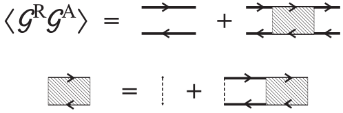
Figure 6: Diagrammatic expansion for the correlation of the Green functions of the disordered system $\langle{\cal G^{R}}{\cal G^{A}}\rangle$.

We are interested in the interactions between the electrons in states sufficiently close to the Fermi surface (within an energy strip $\sim E_{T}$ around the Fermi level). It means that the difference of one-electron eigenenergies entering in the denominators of Eq. (49) are much smaller than $\gamma_{n}$, and can be neglected. Substituting Eq. (49) into Eqs. (32) and (43), and assuming $\left|\varepsilon_{\alpha}-\varepsilon_{\beta}\right|\ll E_{T}$, we find

$$\langle H_{\alpha\beta\gamma\delta}^{(1/g)}\rangle=c_{1}\lambda\frac{\Delta}{g}\left(\delta_{\alpha\delta}\delta_{\beta\gamma}+\delta_{\alpha\gamma}\delta_{\beta\delta}\right);\quad c_{1}=\frac{1}{\pi}\sum_{\gamma_{n}>0}\frac{\gamma_{1}}{\gamma_{n}}\simeq 1,$$ (50)

where the dimensionless conductance of the dot $g$ is defined in Eq. (15). Thus, we have shown that in the metallic regime, $g\gg 1$, the non-universal corrections to the average interaction matrix elements are small indeed.

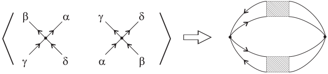
Figure 7: Diagrammatic expansion for the fluctuations of the matrix element in the disordered systems.

Now we turn to the mesoscopic fluctuations $\delta H_{\alpha\beta\gamma\delta}$ of the matrix elements of the interaction Hamiltonian. With the help of Eqs. (32), (43), (37), and of the diagrammatic representation for the disorder average, Fig. 7, one obtains  [67, 69, 66, 68, 70]:

$$\langle\left[\delta H_{\alpha\beta\gamma\delta}^{(1/g)}\right]^{2}\rangle=c_{2}\lambda^{2}\left(\frac{\Delta}{g}\right)^{2},\quad c_{2}=\frac{2}{\pi^{2}}\sum_{\gamma_{m}\neq 0}\left(\frac{\gamma_{1}}{\gamma_{n}}\right)^{2}.$$ (51)

(This result is for the generic case where all indices $\alpha$, $\beta$, $\gamma$, and $\delta$ are different. If they are not all different, the fluctuations are bigger by a number of permutations which that do not change the matrix element. ) Equations (50) and (51) show that the typical deviation of all the matrix elements from their universal values (44) are indeed small as $1/g$.

All the above derivations of the $\propto 1/g$ corrections were performed for diffusive systems. The final estimates in terms of the conductance hold also for ballistic quantum dots with chaotic classical dynamics of electrons, see Appendix A.

2.3.2 RMT for the intra-dot Coulomb interaction

So far, we have shown that the matrix elements of the Hamiltonian of weak, short-range interaction are small compared to $\Delta$. Therefore any observable quantity involving electron states within the energy strip $\sim E_{T}$ around the Fermi level, can be calculated by the lowest-order in $\lambda$ perturbation theory. The situation is different for the long-range Coulomb interaction

$$V(r)=\frac{e^{2}}{\kappa r},$$ (52)

where $\kappa$ is the dielectric constant of the medium containing the electrons of the dot.

For the simplest geometry, the corresponding matrix elements $H_{\alpha\beta\gamma\delta}$ are inversely proportional to the linear size of the dot, rather than to its volume (or area in dimension $d=2$). If the linear size of the dot exceeds the screening radius (or the effective Bohr radius $a_{B}=\kappa\hbar^{2}/e^{2}m^{*}$ in $d=2$), the matrix elements $H_{\alpha\beta\gamma\delta}$ exceed $\Delta$, and the lowest-order perturbation theory in the interaction Hamiltonian fails.

In the theory of linear screening, it is well-known how to deal with this difficulty. When calculating an observable quantity, one should take into account the virtual transitions of low-energy electrons into the high-energy states. If the gas parameter

$$r_{s}\equiv\frac{e^{2}}{\kappa\hbar v_{F}}$$ (53)

(with $v_{F}$ being the electron Fermi velocity) of the electron system in the dot is small, then the random phase approximation (RPA) allows one to adequately account for such virtual transitions. Accounting for these transitions yields, in general, a retarded electron-electron interaction [18]. However, the characteristic scale of the corresponding frequency dependence is of the order of $\gamma_{1}$, see Eq. (11). That is why at the energy scale $|\varepsilon|\>{{}^{{}_{\displaystyle<}}_{\displaystyle\sim}}\>E_{T}$ we can consider the interaction as instantantaneous one, and derive the effective interaction Hamiltonian acting in this truncated space.

A modified matrix element in RPA scheme is shown in Fig. 8. It involves substitution of the bare potential (52) in Eq. (32) with the renormalized potential $V_{\rm sc}\left(\vec{r}_{1},\vec{r}_{2}\right)$. This potential is the solution of the equation

$$V_{\rm sc}\left(\vec{r}_{1},\vec{r}_{2}\right)=V\left(\vec{r}_{1}-\vec{r}_{2}\right)-\int\!\!\int d\vec{r}_{3}d\vec{r}_{4}V\left(\vec{r}_{1}-\vec{r}_{3}\right)\Pi\left(\vec{r}_{3},\vec{r}_{4}\right)V_{\rm sc}\left(\vec{r}_{4},\vec{r}_{2}\right),$$

(54)

where the integration over the intermediate coordinates is performed within the dot only. The polarization operator $\Pi$ should include only the states where at least one electron or (hole) is outside the energy strip of width $\varepsilon^{*}\>{{}^{{}_{\displaystyle<}}_{\displaystyle\sim}}\>E_{T}$ for which we derive the effective Hamiltonian,

$$\Pi\left(\vec{r}_{1},\vec{r}_{2}\right)=2\sum_{|\varepsilon_{\beta}-\varepsilon_{\alpha}|>\varepsilon^{*}}\frac{\phi_{\alpha}(\vec{r}_{1})\phi_{\beta}^{*}(\vec{r}_{1})\phi_{\beta}(\vec{r}_{2})\phi_{\alpha}^{*}(\vec{r}_{2})}{|\varepsilon_{\beta}-\varepsilon_{\alpha}|}\theta(-\varepsilon_{\alpha}\varepsilon_{\beta}).$$ (55)

Here all energies are measured from the Fermi level, and $\theta(x)$ is the step function. The factor of two accounts for spin degeneracy. We can compare Eq. (55) with the usual frequency dependent operator $\Pi^{R}\left(\omega;\vec{r}_{1},\vec{r}_{2}\right)$ that involves all the electron states

$$\Pi^{R}\left(\omega;\vec{r}_{1},\vec{r}_{2}\right)=2\sum_{\varepsilon_{\beta},\varepsilon_{\alpha}}\frac{\phi_{\alpha}(\vec{r}_{1})\phi_{\beta}^{*}(\vec{r}_{1})\phi_{\beta}(\vec{r}_{2})\phi_{\alpha}^{*}(\vec{r}_{2})}{\varepsilon_{\beta}-\varepsilon_{\alpha}-\omega-i0}\theta(-\varepsilon_{\alpha}\varepsilon_{\beta}){\mathrm{s}gn}\varepsilon_{\beta},$$ (56)

and obtain

$$\Pi\left(\vec{r}_{1},\vec{r}_{2}\right)=\frac{1}{\pi}{\mathrm{I}m}\int\frac{d\omega}{\omega}\Pi^{R}\left(\omega;\vec{r}_{1},\vec{r}_{2}\right)\theta\left(|\omega|-\varepsilon^{*}\right).$$ (57)

Figure 8: Matrix element in Random Phase approximation. Polarization operator $\Pi$ involves all the transitions where at least one of the states $\gamma,\ \delta$ is outside the energy strip of the width of the Thouless energy around the Fermi level.

On the next step, we replace the polarization operator with its average value [18]

$$\langle\Pi^{R}\left(\omega;\vec{r}_{1},\vec{r}_{2}\right)\rangle=\frac{2}{\Delta{\cal V}_{d}}\sum_{\gamma_{n}>0}\frac{\gamma_{n}\ f_{n}(\vec{r}_{1})f_{n}(\vec{r}_{2})}{-i\omega+\gamma_{n}},$$ (58)

where $\gamma_{n}$ and $f_{n}$ for a diffusive system are defined in Eq. (11). The prefactor in Eq. (58) is nothing but the thermodynamic density of states per unit volume (area).

Substituting Eq. (58) into Eq. (57) and taking into account that $\varepsilon^{*}\>{{}^{{}_{\displaystyle<}}_{\displaystyle\sim}}\>\hbar\gamma_{1}$, we find

$$\Pi\left(\vec{r}_{1},\vec{r}_{2}\right)=\frac{2}{\Delta{\cal V}_{d}}\sum_{\gamma_{n}>0}f_{n}(\vec{r}_{1})f_{n}(\vec{r}_{2}).$$ (59)

Now we can use the completeness of the solution set of the diffusion equation,

$$\sum_{n}f_{n}({\vec{r}}_{1})f_{n}({\vec{r}}_{2})=\delta({\vec{r}}_{1}-{\vec{r}}_{2}),$$

and the explicit form of the zero-mode solution $f_{0}(\vec{r})=\theta_{\rm dot}(\vec{r})/\sqrt{{\cal V}_{d}}$ for this equation, in order to present Eq. (59) in the form:

$$\Pi\left(\vec{r}_{1},\vec{r}_{2}\right)=\frac{2}{\Delta{\cal V}_{d}}\left[\delta\left(\vec{r}_{1}-\vec{r}_{2}\right)-\frac{1}{{\cal V}_{d}}\right]\theta_{\rm dot}(\vec{r}_{1})\theta_{\rm dot}(\vec{r}_{2}).$$ (60)

Here $\theta_{\rm dot}(\vec{r})=1$, if $\vec{r}$ belongs to the dot and $\theta_{\rm dot}(\vec{r})=0$ otherwise. The structure of Eq. (60) is easy to understand. The first term in brackets characterizes local screening in the Thomas-Fermi approximation. The last term in brackets subtracts the constant-potential contribution of the zero mode which cannot induce electron transitions between the levels and therefore can not be screened.

Substituting the polarization operator (60) in Eq. (54), we find the equation for the self-consistent potential in the Thomas-Fermi approximation:

$$V_{\rm sc}\left(\vec{r}_{1},\vec{r}_{2}\right) = V\left(\vec{r}_{1}-\vec{r}_{2}\right)$$

$$- \frac{2}{\Delta{\cal V}_{d}}\int d\vec{r}_{3}V\left(\vec{r}_{1}-\vec{r}_{3}\right)\left[V_{\rm sc}\left(\vec{r}_{3},\vec{r}_{2}\right)-\frac{1}{{\cal V}_{d}}\int d\vec{r}_{4}V_{\rm sc}\left(\vec{r}_{4},\vec{r}_{2}\right)\right].$$

The use of Thomas-Fermi approximation is justified if the linear size of the dot exceeds the screening radius. The integrals here are taken over the volume of the dot (or over the corresponding area in the $2d$ case). We can rewrite the integral equation (2.3.2) in the more familiar differential form,

$$-\nabla^{2}_{\vec{r}}V_{\rm sc}(\vec{r},\vec{r}_{1}) = \frac{4\pi e^{2}}{\kappa}\left[\delta(\vec{r}-\vec{r}_{1})-\frac{2}{\Delta{\cal V}_{d}^{\vphantom{2}}}\theta_{\rm dot}(\vec{r})V_{\rm sc}(\vec{r},\vec{r}_{1})\right.$$

$$\mbox{}\left.+\frac{2}{\Delta{\cal V}^{2}_{d}}\theta_{\rm dot}(\vec{r})\int d\vec{r}_{2}V_{\rm sc}(\vec{r}_{2},\vec{r}_{1})\theta_{\rm dot}(\vec{r}_{2})\right],$$

supplemented with the requirement that the solution vanishes at $r\to\infty$. In the case of a $2d$ dot, the $\nabla^{2}$ operator is still acting in the three-dimensional space; the right-hand side of Eq. (2.3.2) must be multiplied by $\delta(z)$, where coordinate $z$ is directed normal to the plane of the dot. The second term in the right-hand side of Eq. (2.3.2) represents the familiar Thomas-Fermi screening. In the three-dimensional case, this term is $\propto V_{\rm sc}({\vec{r}})/r_{D}^{2}$, with the screening radius $r_{D}$.

First, we find an approximate solution of Eq. (2.3.2) inside the dot. We consider only length scales larger than the screening radius. This enables us to neglect the left-hand side of Eq. (2.3.2) altogether. In addition, we will neglect the corrections of the order of the level spacing, which are generated by the last term in the right-hand side of Eq. (2.3.2). Then the solution takes the form:

$$V_{\rm sc}(\vec{r},\vec{r}_{1})=\left[\frac{\Delta{\cal V}_{d}}{2}\delta(\vec{r}-\vec{r}_{1})+\bar{V}\right]\theta_{\rm dot}(\vec{r})\theta_{\rm dot}(\vec{r}_{1}),$$ (63)

where the constant $\bar{V}$ will be determined later.

The easiest way to find $\bar{V}$ is to consider Eq. (2.3.2) for $\vec{r}$ outside the dot (keeping $\vec{r}_{1}$ inside the dot). The right-hand side of Eq. (2.3.2) then vanishes,

$$\vec{\nabla}^{2}_{\vec{r}}V_{\rm sc}(\vec{r},\vec{r}_{1})=0.$$ (64)

The constant $\bar{V}$ defines for this Laplace equation the boundary condition at the surface of the dot,

$$V_{\rm sc}(\vec{r},\vec{r}_{1})\big{|}_{\vec{r}\in S}=\bar{V}$$ (65)

(the surface is defined unambiguously in the limit of zero screening radius). After the solution $V_{\rm sc}(\vec{r},\vec{r}_{1})$ of the Laplace equation (64) is found, the constant $\bar{V}$ can be obtained by integration of Eq. (2.3.2) along the surface of the dot:

$$-\oint_{S}d\vec{S}\vec{\nabla}V_{\rm sc}(\vec{r},\vec{r_{1}})=\frac{4\pi e^{2}}{\kappa}.$$ (66)

For the two dimensional case, Eq. (66) obviously reduces to

$$\int d\vec{r}\stackrel{{\scriptstyle\leftrightarrow}}{{\partial}}_{z}V_{\rm sc}(\vec{r},\vec{r}_{1})=\frac{4\pi e^{2}}{\kappa},\quad\stackrel{{\scriptstyle\leftrightarrow}}{{\partial}}_{z}\equiv\left(\frac{\partial}{\partial z}\big{|}_{z\to-0}-\frac{\partial}{\partial z}\big{|}_{z\to+0}\right),$$ (67)

where the two-dimensional integration is performed over the area of the dot ($z=0$).

Now the solution of Eqs. (64) and (65) can be formally found with the help of the Green function of the Laplace equation

$$-\nabla^{2}_{\vec{r}_{1}}{\cal D}(\vec{r}_{1},\vec{r}_{2})=\delta(\vec{r}_{1}-\vec{r}_{2});\quad{\cal D}(\vec{r}_{1},\vec{r}_{2})\big{|}_{\vec{r}_{1}\in S}=0$$ (68)

describing the electrostatic field outside the dot. If the system contains metallic gates, Eq. (68) should be supplied with additional Dirichlet boundary conditions on the surface $S_{i}$ of those gates

$${\cal D}(\vec{r}_{1},\vec{r}_{2})\big{|}_{\vec{r}_{1}\in S_{i}}=0,$$ (69)

where index $i$ enumerates the corresponding gates.

One immediately finds from Eqs. (65) and (68)

$$V_{\rm sc}(\vec{r},\vec{r}_{1})=\bar{V}\oint_{S}d\vec{S}_{2}\vec{\nabla}{\cal D}(\vec{r},\vec{r}_{2})\left[1-\theta_{\rm dot}(\vec{r})\right]$$ (70)

for the potential $V_{\rm sc}$ outside the dot. Substitution of Eq. (70) into Eq. (66) yields

$$\bar{V}=\frac{e^{2}}{C}$$ (71)

for the constant $\bar{V}$. The geometrical capacitance of the dot is given by formula valid for any shape of the dot

$$C=\frac{\kappa}{4\pi}\left|\oint_{S}d\vec{S}_{2}\vec{\nabla_{2}}\oint_{S}d\vec{S}_{1}\vec{\nabla_{1}}{\cal D}(\vec{r}_{1},\vec{r}_{2})\right|.$$ (72)

In a two-dimensional system, Eq. (72) is replaced with

$$C=\frac{\kappa}{4\pi}\left|\int d\vec{r}_{1}\int d\vec{r}_{2}\stackrel{{\scriptstyle\leftrightarrow}}{{\partial}}_{z_{1}}\stackrel{{\scriptstyle\leftrightarrow}}{{\partial}}_{z_{2}}{\cal D}(\vec{r}_{1},\vec{r}_{2})\right|,$$ (73)

where the two-dimensional integration is performed over the area of the dot ($z=0$), and operator $\stackrel{{\scriptstyle\leftrightarrow}}{{\partial}}_{z}$ is defined in Eq. (67). The concrete value of capacitance $C$ is geometry-dependent. If the size of the dot is characterized by a single parameter $L$, then $C$ is proportional to $L$ with some coefficient, which depends on details of the geometry. In the practically important case of a gated dot, the capacitance is $C\simeq L^{2}/4\pi d$, where $L^{2}$ is the area of the dot, and $d\>{{}^{{}_{\displaystyle<}}_{\displaystyle\sim}}\>L$ is the distance from the gate to the plane of the dot.

The charging energy, $e^{2}/2C$, is the dominant energy scale for the matrix elements of the interaction Hamiltonian, as we will now show. Corrections to this scale appear from terms of the order of $\Delta$ in the effective interaction potential $V_{\rm sc}$. In order to find the matrix elements $V_{\alpha\beta\gamma\delta}$, we need to know the screened potential $V_{\rm sc}(\vec{r}_{1},\vec{r}_{2})$ within the dot. The constant part of this potential $\sim e^{2}/C$ contributes only to the “diagonal” matrix elements (32), with $\alpha=\delta$; $\beta=\gamma$. This part does not contribute to any other matrix element, because of the orthogonality of the corresponding one-electron wave functions.

In order to find the non-diagonal matrix elements, we need to account for smaller but coordinate-dependent terms in $V_{\rm sc}(\vec{r}_{1},\vec{r}_{2})$. To accomplish that goal, we substitute the potential (63), (70) into the left-hand side of Eq. (2.3.2) and treat it in the first order of perturbation theory in $\Delta C/e^{2}\ll 1$. As the result, we obtain with the help of Eq. (71)

$$V_{\rm sc}(\vec{r}_{1},\vec{r}_{2})=\frac{e^{2}}{C}+\frac{{\cal V}_{d}\Delta}{2}\delta(\vec{r}_{1}-\vec{r}_{2})+\tilde{V}(\vec{r}_{1})\Delta+\tilde{V}(\vec{r_{2}})\Delta.$$ (74)

Here, the potential $\tilde{V}(\vec{r})$ appears due to the finite size of the dot: a charge $e$ “expelled” from the point $\vec{r}=\vec{r}_{1,2}$ in the process of screening, can not be pushed away to infinity because of the dot’s boundary. In the $3d$ case, this charge forms a thin layer near the boundary of the dot; in the $2d$ case, it creates an inhomogeneous distribution over the whole area of the dot. The explicit form of this potential [in units of level spacing $\Delta$, cf. Eq. (74)] is:

$$\tilde{V}(\vec{r}) = \frac{{\cal V}_{d}}{8\pi C}\oint_{S}\delta(\vec{r}-\vec{r}_{1})d\vec{S}_{1}\vec{\nabla_{1}}\oint_{S}d\vec{S}_{2}\vec{\nabla_{2}}{\cal D}(\vec{r}_{1},\vec{r}_{2});\quad d=3;$$ (75)

$$\tilde{V}(\vec{r}) = \frac{{\cal V}_{d}}{8\pi C}\int d\vec{r}_{1}\stackrel{{\scriptstyle\leftrightarrow}}{{\partial}}_{z}\stackrel{{\scriptstyle\leftrightarrow}}{{\partial}}_{z_{1}}{\cal D}(\vec{r},\vec{r}_{1});\quad d=2,$$

where Green function ${\cal D}(\vec{r},\vec{r}_{1})$ and the dot capacitance $C$ are given by Eqs. (68) and (71), and $\stackrel{{\scriptstyle\leftrightarrow}}{{\partial}}_{z}$ is defined in Eq. (67). The importance of the additional potential (75) for the structure of the matrix elements of the interaction Hamiltonian was first noticed in Ref. [74].

The substitution of the first term of Eq. (74) into Eq. (32) immediately yields the new value of the interaction constant $E_{c}$ in the $\hat{n}$-dependent part of the universal Hamiltonian (35). This constant in fact is the single-electron charging energy:

$$E_{c}=\frac{e^{2}}{2C}.$$ (76)

Note, that this value is much larger than the single electron level spacing:

$$\frac{E_{c}}{\Delta}\simeq r_{s}\left(k_{F}L\right)^{d-1},\quad d=2,3,$$

because of a large factor $k_{F}L\gg 1$. We intend to show now that this large scale appears only in the charge part of the universal Hamiltonian and it enters neither the spin channel nor the non-universal part $\hat{H}_{\rm int}^{(1/g)}$.

The constant $J_{S}$ in Eq. (35) originates from the two-body interaction term of the screened potential. The use of the corresponding (second) term of Eq. (74) would yield $J_{S}=-\Delta/2$, which is an overestimation of the spin-dependent interaction term. The correct result for $J_{S}$ in the random phase approximation reads:

$$-J_{S}=\int d\vec{r}{\cal F}\left(k_{F}|\vec{r}|\right)^{2}V_{\rm sc}(\vec{r})=\frac{\Delta}{\pi}\times\left\{\matrix{r_{s}\ln\left(1+\frac{\pi}{2r_{s}}\right);&\ \ d=3;\cr\frac{r_{s}}{\sqrt{1-r_{s}^{2}}}\ \ln\left(\frac{1+\sqrt{1-r_{s}^{2}}}{1-\sqrt{1-r_{s}^{2}}}\right);&\ \ d=2,}\right.$$

(77)

where the gas parameter $r_{s}$ is given by Eq. (53) and the function ${\cal F}$ was introduced in Eq. (40). It is worthwhile to notice that at $r_{s}\gg 1$, the RPA result (77) gives $J_{S}=-\Delta/2$, which forbids, in particular, the Stoner instability. However, in the regime $r_{s}\>{{}^{{}_{\displaystyle>}}_{\displaystyle\sim}}\>1$, the RPA scheme becomes non-reliable and the constant (77) should be replaced with the corresponding Fermi-liquid constant. A universal description still holds in this case provided that the Fermi liquid description does not breakdown at length scales smaller than the system size.

We now turn to the discussion of $1/g$ corrections. The first type of such corrections results from the substitution of the third and fourth terms of Eq. (74) into Eq. (32). One thus finds [74]:

$$\left[{\cal H}^{(1/g)}_{1}\right]_{\alpha\beta\gamma\delta}=\delta_{\alpha\delta}{\cal X}_{\beta\gamma}^{0}+\delta_{\beta\gamma}{\cal X}_{\alpha\delta}^{0},\quad{\cal X}_{\alpha\beta}^{0}=\int d\vec{r}\tilde{V}(\vec{r})\phi_{\alpha}(\vec{r}_{2})\phi_{\beta}^{*}(\vec{r}_{2}).$$ (78)

The matrix elements in Eq. (78) are random. Their characteristic values can be easily found from Eqs. (74) and (49), with the result

$$\langle\left[{\cal X}^{0}_{\alpha\beta}\right]^{2}\rangle=b_{00}\frac{\Delta^{2}}{g},$$ (79)

where $b_{00}$ is a geometry dependent numerical coefficient,

$$b_{00}=\frac{1}{\pi}\sum_{\gamma_{n}>0}\frac{\left|\int d\vec{r}\tilde{V}(\vec{r})f_{n}(\vec{r})\right|^{2}\gamma_{1}}{\gamma_{n}},$$ (80)

and the potential $\tilde{V}$ is defined by Eq. (75). The coefficient $b_{00}$ is of the order of unity. According to Eq. (78), the matrix elements $\left[{\cal H}^{(1/g)}\right]_{\alpha\beta\gamma\delta}$ of the Hamiltonian $\hat{H}^{1/g}$ with $\alpha=\delta$ or $\beta=\gamma$ are of the order of $\Delta/\sqrt{g}$, contrary to the assumptions of Ref. [75]. The rest of these matrix elements are smaller. One can use the two-body part of the screened interaction potential (74) to evaluate them [67]. This part coincides with the simple model (43), up to the constant $\lambda$, which should be substituted by $1/2$. After the substitution, one can use the results (50) and (51).

In all the previous consideration, we assumed the potential on the external gates to be fixed, see Eq. (69). Such an assumption was valid because additional potentials created by those gates were implicitly included into the confining potential $U(\vec{r})$ from Eq. (1). One, however, may be interested in a comparison of the properties of the dot at two different sets of the gate voltages. To address such a problem one has to include gates into the electrostatic problem, i.e., to find the correction $\delta U(\vec{r})$ to the self-consistent confining potential due to the variation of the gate potentials. This requires that the Thomas - Fermi screening of the charge on the external gates by the electrons in the dot has to be considered. The resulting equation for this correction is similar to Eq. (2.3.2):

$$-\nabla^{2}\delta U(\vec{r})=-\frac{2}{\Delta{\cal V}_{d}}\left[\theta_{\rm dot}(\vec{r})\delta U(\vec{r})-\frac{1}{{\cal V}_{d}}\int d\vec{r}_{1}\theta_{\rm dot}(\vec{r}_{1})\delta U(\vec{r}_{1})\right],$$ (81)

supplemented with the requirement that the solution vanishes at $r\to\infty$ and has the fixed value on the surface of each gate, $S_{i}$, [compare with Eq. (69)]:

$$\delta U(\vec{r})\big{|}_{\vec{r}\in S_{i}}=-eV_{g}^{(i)},\quad i=1,2,\dots,$$ (82)

where indices $i$ enumerate the gates, and $V_{g}^{(i)}$ is the electrostatic potential on $i$-th gate.

Solving Eqs. (81) – (82) involves the same steps as in derivation of Eq. (74) [the only difference is that now there is no $\delta$-function in Eq. (63), the right hand side of Eq. (66) vanishes, and the boundary conditions on the gate surfaces are given by Eq. (82)]. The solution for the potential outside the dot is obtained in terms of the Green function (68) – (69), similarly to Eq. (70):

$$\delta U(\vec{r})=\delta\bar{U}\oint_{S}d\vec{S}_{2}\vec{\nabla}{\cal D}(\vec{r},\vec{r}_{2})-\sum_{i}eV_{g}^{(i)}\oint_{S_{i}}d\vec{S}_{2}\vec{\nabla}{\cal D}(\vec{r},\vec{r}_{2}),$$ (83)

where the zero-mode part of the potential of the dot is given by

$$\delta\bar{U}=-2E_{c}{\cal N},\quad{\cal N}=\sum_{i}{\cal N}_{i},\quad e{\cal N}_{i}=C_{i}V_{g}^{(i)}.$$ (84)

The geometrical capacitance of the dot $C$ is defined by Eqs. (72) and (73) and the geometrical mutual capacitances between the dot and the gates are

$$C_{i}=\frac{\kappa}{4\pi}\oint_{S_{i}}d\vec{S}_{2}\vec{\nabla_{2}}\oint_{S}d\vec{S}_{1}\vec{\nabla_{1}}{\cal D}(\vec{r}_{1},\vec{r}_{2}),$$ (85)

for three-dimensional dots. To obtain the result for the two-dimensional case, the surface integral over $S$ here should be replaced as in Eq. (67). The resulting potential inside the dot is found similarly to Eq. (74) in the form

$$\delta U(\vec{r})=-2E_{c}{\cal N}-\Delta\left[{\cal N}\tilde{V}(\vec{r})+\sum_{i}{\cal N}_{i}\tilde{V}^{(i)}(\vec{r})\right],$$ (86)

where $\tilde{V}(\vec{r})$ is defined in Eq. (75) and potentials $\tilde{V}^{(i)}(\vec{r})$ are given by

$$\tilde{V}^{(i)}(\vec{r}) = \frac{{\cal V}_{d}}{8\pi C_{i}}\oint_{S}\delta(\vec{r}-\vec{r}_{1})d\vec{S}_{1}\vec{\nabla_{1}}\oint_{S_{i}}d\vec{S}_{2}\vec{\nabla_{2}}{\cal D}(\vec{r}_{1},\vec{r}_{2});\quad d=3;$$ (87)

$$\tilde{V}^{(i)}(\vec{r}) = \frac{{\cal V}_{d}}{8\pi C_{i}}\int_{S_{i}}d\vec{r}_{1}\stackrel{{\scriptstyle\leftrightarrow}}{{\partial}}_{z}\stackrel{{\scriptstyle\leftrightarrow}}{{\partial}}_{z_{1}}{\cal D}(\vec{r},\vec{r}_{1});\quad d=2.$$

We see that the effect of the external gates has the same hierarchical structure as the electronic interaction inside the dot: The largest scale $E_{c}$ [the first term in Eq. (86)] corresponds to a simple uniform shift of the potential, while the much smaller energy scale $\Delta$ characterizes the changes in the potential affecting the shape of the dot. Therefore, the effect of the external gates can be separated into a universal part $\delta U^{0}$ and a fluctuating non-universal part $\delta U^{1/g}$:

$$\delta U^{0}_{\alpha\beta}=-2E_{c}{\cal N}\delta_{\alpha\beta};$$ (88)

$$U^{(1/g)}_{\alpha\beta}=-{\cal N}{\cal X}^{0}_{\alpha\beta}-\sum_{j}{\cal N}_{j}{\cal X}^{j}_{\alpha\beta}.$$ (89)

In Eq. (89), the ${\cal X}^{j}_{\alpha\beta}$ are random Gaussian variables with second moments

$$\langle{\cal X}^{i}_{\alpha\beta}{\cal X}^{j}_{\alpha\beta}\rangle=b_{ij}\frac{\Delta^{2}}{g},$$ (90)

where the geometry dependent coefficient $b_{00}$ is given by Eq. (80) and all other coefficients are given by

$$b_{ij}=\frac{1}{\pi}\sum_{\gamma_{n}>0}\frac{\gamma_{1}}{\gamma_{n}}\int d\vec{r}\tilde{V}^{(i)}(\vec{r})f_{n}(\vec{r})\int d\vec{r}\tilde{V}^{(j)}(\vec{r})f_{n}(\vec{r}),$$ (91)

$$b_{0j}=b_{j0}=\frac{1}{\pi}\sum_{\gamma_{n}>0}\frac{\gamma_{1}}{\gamma_{n}}\int d\vec{r}\tilde{V}(\vec{r})f_{n}(\vec{r})\int d\vec{r}\tilde{V}^{(j)}(\vec{r})f_{n}(\vec{r})$$

for $i,j=1,2\dots$. In general all these coefficients are of the order of unity.

2.3.3 Final form of the effective Hamiltonian

To summarize this subsection, we note that in the absence of superconducting correlations, the universal part of the interaction Hamiltonian, Eq. (35), consists of two parts. The dominant part depends on the dot’s charge $\hat{n}$. The corresponding energy scale $E_{c}$, Eq. (76), is related to the geometric capacitance of the dot $C$, Eq. (72), and exceeds parametrically the level spacing $\Delta$. [There are corrections of order $\Delta$ to Eq. (76) arising from the potentials $\tilde{V}$ in Eq. (74) and from the local part of the screened interaction.] The next part depends on the total spin $\vec{S}$ of the dot. The corresponding energy scale $J_{S}$ is smaller than $\Delta$. If the level spacing did not fluctuate, then the smallness of $J_{S}$ would automatically mean that the spin of the dot $S=0$ or $S=1/2$ depending on whether the number of electrons in the dot is even or odd, respectively. Fluctuations of the level spacing may lead to a violation of the strict periodicity in this dependence [76, 77, 78]. However, the Stoner criterion [79] guarantees that the spin of the dot is not macroscopically large (i.e.,, does not scale with the volume of the dot). The strongest non-universal correction to the Hamiltonian (35) comes from the effect of the boundary of the dot on the interaction potential, see Eq. (74), and is of the order of $\Delta/\sqrt{g}$, where $g$ is the dimensionless conductance of the dot (15). In the presence of the gate, the universal part $\hat{H}^{(0)}$ of the Hamiltonian (including the RMT representation (13) of its free-electron part) and the two largest non-universal corrections $\hat{H}^{1/g}$ have the following form:

$$\hat{H}^{(0)}=\sum_{\alpha,\gamma}{\cal H}_{\alpha\gamma}\psi^{\dagger}_{\alpha,\sigma}\psi_{\gamma,\sigma}+E_{c}\left(\hat{n}-{\cal N}\right)^{2}+J_{S}\left(\hat{\vec{S}}\right)^{2}-E_{c}{\cal N}^{2},$$ (92)

$$\hat{H}^{(1/g)}=\sum_{\alpha,\beta}\psi^{\dagger}_{\alpha,\sigma}\psi_{\beta,\sigma}\left[\left(\hat{n}-{\cal N}\right){\cal X}_{\alpha\beta}^{0}-\sum_{j}{\cal N}_{j}{\cal X}_{\alpha\beta}^{j}\right]$$

$$\quad\quad\quad\quad+\frac{1}{2}\sum_{\alpha\beta\gamma\delta}{\cal H}_{\alpha\beta\gamma\delta}^{(1/g)}\psi^{\dagger}_{\alpha,\sigma_{1}}\psi^{\dagger}_{\beta,\sigma_{2}}\psi_{\gamma,\sigma_{2}}\psi_{\delta,\sigma_{1}}.$$ (93)

The last term in Eq. (92) is a $c$-number and it can be disregarded in all subsequent considerations. The fluctuations of the matrix matrix elements ${\cal X}_{\alpha\beta}^{(j)}$ are given by Eq. (90), the elements ${\cal H}_{\alpha\beta\gamma\delta}^{(1/g)}$ can be estimated from Eqs. (50) and (51) with $\lambda=1/2$. Finally we should mention that for a two-dimensional dot the relation $E_{c}\gg\Delta$ holds only if the distance between the dot and gate exceeds the screening radius in the dot.

2.4 Inclusion of the leads

So far we considered an isolated dot. We have established the validity of the universal RMT description both for the one electron Hamiltonian and for the interaction effects. Our goal now is to present a similar description for the connection of the dot with the external leads.

We will assume that the leads contacting the dot are sufficiently clean, and neglect the mesoscopic fluctuations of the local density of states in the leads. In other words, we neglect closed electron trajectories in the leads that start at the contacts. We also neglect the electron-electron interaction in the leads. In the case of two-dimensional leads, this approximation is justified if the dimensionless conductance of the leads greatly exceeds the number of channels in the point contacts connecting leads to the quantum dot, or, equivalently, when the resistance of the leads is much smaller than the conductance of the point contacts.

We wish to keep the RMT description of the dot. On the other hand, we saw that it is justified only for energy scales much smaller than Thouless energy $E_{T}=g\Delta$, where $g$ is the dimensionless conductance of the dot. The presence of point contacts with a total number of propagating modes $N_{\rm ch}$ broadens each level by an amount of the order of $N_{\rm ch}\Delta$. Hence, the use of the RMT description requires the condition

$$N_{\rm ch}\ll g,$$ (94)

where the dimensionless conductance of the dot is defined by Eq. (15). Since $g\gg 1$, the condition (94) is met even if more than one channel is open.

The conductance of a point contact connecting two clean conducting continua can be related, by the Landauer formula  [80, 81, 82, 83, 84], to a scattering problem for electron waves incident on the contact. These waves can be labeled by a continuous wave number $k$ and by a set of discrete quantum numbers $j$. The number $k$ accounts for the continuous energy spectrum of the incoming waves, and $j$ defines their spatial structure in the directions transverse to the direction of incidence. Although in principle the number of discrete modes $j$ participating in scattering is infinite, the number of relevant modes contributing to the conductance is confined to the $N_{\rm ch}$ modes that are propagating through the contact; all other modes are evanescent and hardly contribute to the conductance. An adiabatic point contact [5, 10, 85] is an example adequately described by a model having $N_{\rm ch}$ modes in a lead.

Let us now turn to a quantitative description of the theory. The total Hamiltonian of the system is given as a sum of three terms [86],

$$\hat{H}_{t}=\hat{H}+\hat{H}_{L}+\hat{H}_{LD},$$ (95)

where the Hamiltonian of the closed dot, $\hat{H}$, will be taken in the universal limit, see Eq. (92), $\hat{H}_{L}$ describes the leads, and $\hat{H}_{LD}$ couples the leads and the dot. A separation into three terms, like Eq. (95), is well known in the context of the tunneling Hamiltonian formalism [87], and in nuclear physics [88]. Its application to point contacts coupling to quantum dots can be found, e.g., in Refs. [14, 86, 89, 90]. The Hamiltonian of the leads reads

$$\hat{H}_{L}=v_{F}\sum_{j=1}^{N_{\rm ch}}\int\frac{dk}{2\pi}k\hat{\psi}^{\dagger}_{j}(k)\hat{\psi}_{j}(k),$$ (96)

where we have linearized the electron spectrum in the leads and measure all the energies from the Fermi level. The vector $k\ll k_{F}$ is the deviation of longitudinal momentum in a propagating mode from the Fermi wavevector $k_{F}$. [For the sake of simplicity, we assume the Fermi velocity to be the same in all the modes; the general case can be reduced to Eq. (96) by a simple rescaling.] The Hamiltonian (96) accounts for all the leads attached to the dot; the lead index (in case the dot is coupled to more than one lead), the transverse mode index, and the spin index have all been combined into the single index $j$, which is summed from $1$ to $N_{\rm ch}$, $N_{\rm ch}$ being the total number of propagating channels in all the leads. (In this subsection, we reserve Greek and Latin letters for labelling the fermionic states in the dot and in the leads respectively.)

The Hamiltonian $\hat{H}_{LD}$ in Eq. (95) describes the coupling of the dot to the leads,

$$\hat{H}_{LD}=\sum_{j=1}^{N_{\rm ch}}\sum_{\alpha=1}^{M}\int\frac{dk}{2\pi}\left[W_{\alpha j}\psi^{\dagger}_{\alpha}\psi_{j}(k)+{\rm h.c.}\right].$$ (97)

Here the coupling constants $W_{\alpha j}$ form a real $M\times N_{\rm ch}$ matrix $W$, and $M\to\infty$ is the size of the random matrix describing the Hamiltonian of the dot. We emphasize that the matrix $W$ describes the point contacts, not the dot. That is why this matrix is not random: all the randomness is included in the matrix ${\cal H}$ from Eq. (92).

In the absence of electron-electron interactions in the dot, the Hamiltonian (95) of the combined system of dot and leads can be easily diagonalized and the one-electron eigenstates can be found. These eigenstates are best described by the $N_{\rm ch}\times N_{\rm ch}$ scattering matrix $S(\varepsilon)$, which relates the amplitudes $a^{\rm out}_{j}$ of out-going waves and $a^{\rm i}_{j}$ of in-going waves in the leads,

$$a_{i}^{\rm out}=\sum_{j=1}^{N_{\rm ch}}S_{ij}(\varepsilon)a_{j}^{\rm in}.$$ (98)

(For a precise definition of the amplitudes $a_{j}^{\rm in}$ and $a_{j}^{\rm out}$ in terms of the lead states $\psi_{j}(k)$, and for a derivation of the formulae presented below, we refer to appendix C.) The matrix $S$ is unitary, as required by particle conservation. It can be expressed in terms of the matrices $W$ and ${\cal H}$ that define the non-interacting part of the Hamiltonian and a matrix $U$ that describes the boundary condition at the lead-dot interface,

$$S(\varepsilon)=U\left[1-2\pi i\nu W^{\dagger}\left({\varepsilon-{\cal H}+i\pi\nu WW^{\dagger}}\right)^{-1}W\right]U^{\rm T},$$ (99)

where $\nu=1/(2\pi v_{F})$ is the one-dimensional density of states in the leads, the $M\times M$ matrix ${\cal H}$ is formed by the elements ${\cal H}_{\alpha\gamma}$ of the Hamiltonian of the dot (92), and $UU^{\rm T}$ is the scattering matrix in the absence of the coupling between the leads and the dot (i.e., when $H_{LD}=0$). The scattering matrix $S_{ij}(\varepsilon)$ describes scattering of electrons from one lead to another, as well as backscattering of an electron into the same lead. Equation (99) can be also rewritten in terms of the (matrix) Green function of the closed dot

$${\cal G}(\varepsilon)=(\varepsilon-{\cal H})^{-1},$$ (100)

as

$$S(\varepsilon)=U\frac{1-i\pi\nu W^{\dagger}{\cal G}(\varepsilon)W}{1+i\pi\nu W^{\dagger}{\cal G}(\varepsilon)W}U^{\rm T}.$$ (101)

The matrix $S$ describes both reflection from the point contacts (i.e., scattering processes that involve the backscattering from the contacts only, not the dot), and scattering that involves (ergodic) exploration of the dot. Alternatively, the backreflection from the point contacts into the leads can be described in terms of a reflection matrix $r_{c}$, which is related to the matrix $W$ as

$$r_{c}=U{\pi^{2}\nu-M\Delta W^{\dagger}W\over\pi^{2}\nu+M\Delta W^{\dagger}W}U^{\rm T}.$$ (102)

A contact is called ideal if $r_{c}=0$, or, equivalently, $W^{\dagger}W=\pi^{2}\nu/M\Delta$. For a single mode contact, the transparency $|t_{c}|^{2}$ is given by $|t_{c}|^{2}=1-|r_{c}|^{2}$.

For non-interacting electrons Eqs. (99) – (102) essentially solve the physical part of the problem since all the observable quantities are expressed in terms of the scattering matrix. We now consider three observables in more detail: the two-terminal conductance, the tunneling density of states, and the ground state energy of the dot in contact to the leads.

Two-terminal conductance. The two-terminal conductance is defined for a quantum dot that is connected to electron reservoirs via two leads (numbered $1$ and $2$) with $N_{1}$ and $N_{2}$ channels each (where $N_{1}+N_{2}=N_{\rm ch}$), see Fig. 9. The electron reservoirs are held at a constant chemical potential $\mu+eV_{i}$ ($i=1,2$). Labeling the group of channels belonging to lead $1$ ($2$) with the index $1\leq j\leq N_{1}$ ($N_{1}+1\leq j\leq N_{\rm ch}$), the total current $I$ through, say, lead no. $1$ is given by

$$I=G\left(V_{2}-V_{1}\right),$$

where the conductance $G$ is expressed in terms of the scattering matrix $S$ by the Landauer formula [93, 80, 81, 82]

$$G=\frac{e^{2}}{2\pi\hbar}\int d\varepsilon\left(-\frac{\partial f_{F}}{\partial\varepsilon}\right)\sum_{i=1}^{N_{1}}\sum_{j=N_{1}+1}^{N_{\rm ch}}\left|S_{ij}(\varepsilon)\right|^{2},$$ (103)

$f_{F}(\varepsilon)=1/(1+e^{\varepsilon/T})$ being the Fermi distribution function.

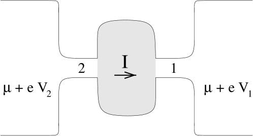
Figure 9: Setup for a measurement of the two-terminal conductance. The quantum dot (grey) is connected to two leads, numbered $1$ and $2$, that are connected to electron reservoirs. A current $I$ flows through the dot as a function of the voltage difference $V_{1}-V_{2}$ between the reservoirs.

It is convenient to use the unitarity of the scattering matrix and rewrite Eq. (103) as

$$G=\frac{e^{2}}{2\pi\hbar}\left[\frac{N_{1}N_{2}}{N_{\rm ch}}-\int d\varepsilon\left(-\frac{\partial f_{F}}{\partial\varepsilon}\right){\rm Tr}\Lambda S\Lambda S^{\dagger}\right],$$ (104)

where the $N_{\rm ch}\times N_{\rm ch}$ traceless matrix $\Lambda$ is defined as

$$\Lambda_{ij}=\delta_{ij}\times\left\{\begin{array}[]{ll}-\displaystyle{N_{2}\over N_{\rm ch}\vphantom{M_{M}}},&i=1,\dots,N_{1},\\ \hphantom{-}\displaystyle{N_{1}^{\vphantom{M_{M}}}\over N_{\rm ch}},&i=N_{1}+1,\dots,N_{\rm ch}.\end{array}\right.$$ (107)

The advantage of Eq. (104) over the more conventional form (103) of the Landauer formula is that it separates the classical conductance $(2e^{2}/h)(N_{1}N_{2}/N_{\rm ch})$ and the quantum interference correction, the second term on the r.h.s. of Eq. (104).

Tunneling density of states. An important particular case of Eq. (103) is the strongly asymmetric setup, where one of the contacts, say the right one (no. $1$ in Fig. 9), has only one channel ($N_{1}=1$), with a very small transmission amplitude, $|t_{c}|^{2}=1-|r_{c}|^{2}\ll 1$. The corresponding coupling matrix $W$ from Eq. (97) then acquires the form, see also Eq. (102)

$$W_{\alpha j}=\delta_{\alpha j}\delta_{\alpha 1}\frac{t_{c}}{2}\sqrt{\frac{\Delta M}{\pi^{2}\nu}}+\left(1-\delta_{1j}\right)W_{\alpha j}^{(2)}.$$ (108)

Here the channel $j=1$ corresponds to the right contact, while the channels $j=2,\ldots,N_{\rm ch}$ correspond to the left contact, and we have chosen the basis of the states inside the dot such that the right contact is connected to “site” $\alpha=1$. The matrix $W_{\alpha j}^{(2)}$ describes the coupling to the left contact. Substituting Eq. (108) into Eq. (99) and using Eq. (108) one obtains, with the help of Eq. (103)

$$G=G_{1}\Delta M\int d\varepsilon\left(-\frac{\partial f_{F}}{\partial\varepsilon}\right)\nu_{T}(\varepsilon),$$ (109)

where the tunneling conductance of the left contact is given by

$$G_{1}=\frac{e^{2}}{\pi\hbar}|t_{c}|^{2}.$$

The quantity $\nu_{T}(\varepsilon)$ in Eq. (109) is the tunneling density of states and is given by (in the next two formulae we omit the superscript $(2)$ in $\hat{W}^{(2)}$):

$$\nu_{T}(\varepsilon) = \nu\left[\frac{1}{\varepsilon-{\cal H}+i\pi\nu WW^{\dagger}}WW^{\dagger}\frac{1}{\varepsilon-{\cal H}-i\pi\nu WW^{\dagger}}\right]_{11}$$ (110)

$$= -\frac{1}{\pi}\mbox{Im}\,\left[\frac{1}{\varepsilon-{\cal H}+i\pi\nu WW^{\dagger}}\right]_{11}$$

$$= -\frac{1}{\pi}\mbox{Im}\left[{\cal G}_{o}^{R}(\varepsilon)\right]_{11},$$

a result which one can obtain also by treating the right contact in the tunneling Hamiltonian approximation. Here, we introduced the Green functions for the dot connected to the leads, cf. Eq. (100)

$${\cal G}_{o}^{R(A)}=\left[\varepsilon-{\cal H}\pm i\pi\nu WW^{\dagger}\right]^{-1},$$ (111)

where the “$+$” (“$-$”) sign corresponds to the retarded (advanced) Green functions respectively.

An equivalent form of Eq. (110) is obtained by noticing from Eq. (100) that $\partial{\cal G}_{\alpha\beta}/\partial{\cal H}_{11}={\cal G}_{\alpha 1}{\cal G}_{1\beta}$. One immediately finds from Eq. (110)

$$\nu_{T}(\varepsilon)=\frac{1}{2\pi i}\frac{\partial}{\partial{\cal H}_{11}}{\mathrm{T}r}\ln\left(\frac{1+i\pi\nu W^{\dagger}{\cal G}(\varepsilon)W}{1-i\pi\nu W^{\dagger}{\cal G}(\varepsilon)W}\right),$$

and with the help of Eq. (101) and $SS^{\dagger}=1$, arrives at [94]

$$\nu_{T}(\varepsilon)=-\frac{1}{2\pi i}{\mathrm{T}r}S^{\dagger}\frac{\partial{S}}{\partial{\cal H}_{11}}.$$ (112)

This indicates that the tunneling density of states can be related to the parametric derivative of the scattering matrix of the dot without the left (tunneling) contact.

Free energy for non-interacting electrons. The thermodynamic potential $\Omega$ of the dot at chemical potential $\mu$ can be found in terms of the Green functions as

$$\Omega=-{T}\int d\varepsilon\ln\left[1+e^{-(\varepsilon-\mu)/T}\right]\,\nu(\varepsilon),$$ (113)

where the total density of states (i.e., the local density of states integrated over the volume of the dot) $\nu(\varepsilon)$ is given by [compare with Eq. (110)]

$$\nu(\varepsilon)=-{1\over\pi}\mbox{Im}\,{\mathrm{T}r}\frac{1}{\varepsilon-{\cal H}+i\pi\nu WW^{\dagger}}.$$ (114)

Similarly to the derivation of Eq. (112), one can rewrite the latter formula in terms of the energy derivative of the scattering matrix as [94]

$$\nu(\varepsilon)={1\over 2\pi i}{\mathrm{T}r}\,S^{\dagger}\frac{\partial{S}}{\partial\varepsilon}$$ (115)

The average number of particles in the dot $\langle\hat{n}\rangle_{q}=-\partial\Omega/\partial\mu$ (here $\langle\dots\rangle_{q}$ indicates the average over the quantum state without disorder average) can then be found as

$$\langle\hat{n}\rangle_{q}=\int d\varepsilon f_{F}(\varepsilon)\nu(\varepsilon),$$ (116)

where $f_{F}(\varepsilon)$ is the Fermi function.

Statistical properties of $S$. The calculation of the statistical properties of the two-terminal conductance, the tunneling density of states, and the ground state energy is now reduced to the analysis of the properties of the scattering matrix for a chaotic quantum dot, which is a doable, though not straightforward task. The available results are collected in an excellent review  [14] (see, in particular, Ch. 2 of that reference). Here, we mention a few results that are needed in Sec. 4. For particles with spin, but in the absence of spin-orbit scattering, the scattering matrix is block diagonal, $S=\mbox{diag}\,(S^{o},S^{o})$, where each block $S^{o}$ is a matrix of size $N_{\rm ch}^{o}=N_{\rm ch}/2$, the total number of orbital channels. In the presence of spin-orbit scattering such a block structure does not exist, and one commonly describes $S$ as a $N_{\rm ch}^{o}$-dimensional matrix of quaternions (denoted as $S^{o}$), which are $2\times 2$ matrices with special rules for complex conjugation and transposition [54]. For reflectionless contacts all averages that involve $S$ (or $S^{\dagger}$) only vanish,

$$\langle S_{i_{1}j_{1}}(\varepsilon_{1})S_{i_{2}j_{2}}(\varepsilon_{2})\ldots S_{i_{n}j_{n}}(\varepsilon_{n})\rangle=0,\ \ n=1,2,\ldots.$$ (117)

For nonideal contacts, the average of $S$ does not vanish, and is given by the reflection matrix $r_{c}$ of the contact,

$$\langle S_{i_{1}j_{1}}(\varepsilon_{1})S_{i_{2}j_{2}}(\varepsilon_{2})\ldots S_{i_{n}j_{n}}(\varepsilon_{n})\rangle=\prod_{k=1}^{n}r_{c,i_{k}j_{k}},\ \ n=1,2,\ldots.$$ (118)

Moments that involve both $S$ and $S^{\dagger}$ have a rather complicated dependence on energy (see, e.g., Ref. [95] for $\beta=1$). Here, we mention an approximate result for the second moment $\langle{S^{o}_{i_{1}j_{1}}(\varepsilon_{1})S^{o*}_{i_{2}j_{2}}(\varepsilon_{2})}\rangle$ in case $r_{c}=0$,

$$\langle{S^{o}_{i_{1}j_{1}}(\varepsilon_{1})S^{o*}_{i_{2}j_{2}}(\varepsilon_{2})}\rangle = \frac{\delta_{i_{1}i_{2}}\delta_{j_{1}j_{2}}+(2/\beta-1)\delta_{i_{1}j_{2}}\delta_{j_{1}i_{2}}}{N_{\rm ch}^{o}+2/\beta-1+2\pi i(\varepsilon_{2}-\varepsilon_{1})/\Delta},$$ (119)

where $\Delta$ is the mean level spacing of the dot. The approximation (119) is valid for $\varepsilon_{1}-\varepsilon_{2}=0$ and for large values of $|\varepsilon_{2}-\varepsilon_{1}|\gg\Delta$. It is also valid for arbitrary $|\varepsilon_{1}-\varepsilon_{2}|$ if $N_{\rm ch}\gg 1$. This is sufficient to estimate average and fluctuation properties of the conductance for temperatures $T\gg N_{\rm ch}\Delta$ (see Sec. 4).

If $r_{c}$ is nonzero, one finds

$$\langle{S^{o}_{i_{1}j_{1}}(\varepsilon_{1})S^{o*}_{i_{2}j_{2}}(\varepsilon_{2})}\rangle = (r_{c})_{i_{1}j_{1}}^{\vphantom{\dagger}}(r_{c})^{*}_{i_{2}j_{2}}$$ (120)

$$\mbox{}+{(1-r_{c}^{\vphantom{\dagger}}r_{c}^{\dagger})_{i_{1}i_{2}}(1-r_{c}^{\dagger}r_{c}^{\vphantom{\dagger}})_{j_{1}j_{2}}\over N_{\rm ch}^{o}+2/\beta-1-\mbox{Tr}\,r_{c}r_{c}^{\dagger}+2\pi i(\varepsilon_{2}-\varepsilon_{1})/\Delta}$$

$$\mbox{}+{(2/\beta-1)(1-r_{c}^{\vphantom{\dagger}}r_{c}^{\dagger})_{i_{1}j_{2}}(1-r_{c}^{\dagger}r_{c}^{\vphantom{\dagger}})_{j_{1}i_{2}}\over N_{\rm ch}^{o}+2/\beta-1-\mbox{Tr}\,r_{c}^{\vphantom{\dagger}}r_{c}^{\dagger}+2\pi i(\varepsilon_{2}-\varepsilon_{1})/\Delta}.$$

This approximate result is for large energy differences or for the case $N_{\rm ch}-\mbox{Tr}\,r_{c}^{\vphantom{\dagger}}r_{c}^{\dagger}\gg 1$.

In Sec. 4 we use the Fourier transform $S(t)$ of the scattering matrix,

$$S(\varepsilon)=\int_{0}^{\infty}dtS(t)e^{i\varepsilon t},$$ (121)

for $\varepsilon$ in the upper half of the complex plane. The Fourier transform of the hermitian conjugate is defined with negative times and for $\varepsilon$ in the lower half of the complex plane,

$$S^{\dagger}(\varepsilon)=\int_{0}^{\infty}dtS^{\dagger}(-t)e^{-i\varepsilon t}.$$ (122)

Statistical averages for the scattering matrix in time-representation can be obtained by Fourier transform of Eqs. (117) – (119), recalling that ensemble and energy averages are equivalent. In particular, we find that the scattering from a nonideal point contact with energy-independent $r_{c}\neq 0$ is instantaneous,

$$S(t)=r_{c}\,\delta(t)+\mbox{fluctuating part},$$ (123)

where the reflection matrix of the point contact $r_{c}$ is defined in Eq. (LABEL:eq:2.620), and the ensemble average of the “fluctuating part” (and of its integer powers) vanishes, see Eq. (118). For the correlator of $S(t_{1})$ and $S^{\dagger}(t_{2})$ for $r_{c}=0$, we find from Eq. (119)

$$\langle{S^{o}_{i_{1}j_{1}}(t_{1})S^{o*}_{i_{2}j_{2}}(t_{2})}\rangle = \frac{\Delta}{2\pi}\left[\delta_{i_{1}i_{2}}\delta_{j_{1}j_{2}}+(2/\beta-1)\delta_{i_{1}j_{2}}\delta_{j_{1}i_{2}}\right]$$ (124)

$$\mbox{}\times\delta(t_{1}+t_{2})e^{-(N_{\rm ch}+2/\beta-1)t_{1}\Delta/(2\pi)},$$

where $\beta=1(2,4)$ corresponds to the orthogonal (unitary, symplectic) ensemble.

Statistical properties of ${\cal G}_{o}$. We will see in Section 4.8, that the tunneling conductance in the presence of the interaction can not be expressed in terms of the parametric derivative of $S$, as it was done in Eq. (112). The transport in this case will be related to the statistics of the Green functions for the open dot (111), and we give those properties below. It is more convenient to write the results in the time domain. For averages which include only retarded or only advanced components one finds

$$\langle\left[{\cal G}^{R}_{o}(t)\right]_{\alpha\gamma}\rangle=-\langle\left[{\cal G}^{A}_{o}(t)\right]_{\alpha\gamma}\rangle=-i\delta(t)\delta_{\alpha\gamma}\frac{\pi}{\Delta M},$$

$$\langle\prod_{j}{\cal G}^{R}_{o}(t_{j})\rangle=\prod_{j}\langle{\cal G}^{R}_{o}(t_{j})\rangle,$$ (125)

which means that the attachment of the leads does not change the average level spacing in the dot. For averages involving the retarded and advanced components, we have for the case of reflectionless contacts

$$\langle\left[{\cal G}^{R}_{o}(t_{1})\right]_{\alpha_{1}\gamma_{1}}\left[{\cal G}^{A}_{o}(t_{2})\right]_{\alpha_{2}\gamma_{2}}\rangle = \frac{2\pi}{M^{2}\Delta}\left[\delta_{\alpha_{1}\gamma_{2}}\delta_{\alpha_{2}\gamma_{1}}+(2/\beta-1)\delta_{\alpha_{1}\gamma_{1}}\delta_{\alpha_{2}\gamma_{1}}\right]$$ (126)

$$\mbox{}\times\delta(t_{1}+t_{2})e^{-(N_{\rm ch}+2/\beta-1)t_{1}\Delta/(2\pi)}.$$

The derivation of Eq. (126) may be performed similar to that of Eq. (25).

This concludes our brief review of the two-terminal conductance, the tunneling density of states, and the ground state energy for a quantum dot in the absence of electron-electron interactions. The interaction between electrons leads to the Coulomb blockade, and simple formulas as Eq. (103), (112), and (115) cease to be valid. With interactions, the answer very substantially depends on the conductance of the dot-lead junctions. The consideration of this regime will be the subject of the two remaining sections.

3 Strongly blockaded quantum dots

In this Section, we discuss the regime of strong Coulomb blockade in quantum dots. To allow for this regime, the conductances of the contacts of the dot to the leads $G_{1,2}$ must be small in units of $e^{2}/\pi\hbar$. As it was already explained in the Introduction, junctions to a quantum dot formed in a two-dimensional electron gas of a semiconductor heterostructure are well described by the adiabatic point contact model. Normally, a small conductance is realized only in single-mode junctions. Since there are two leads connected to the dot, labeled $1$ and $2$, we have total number of (orbital) channels $N_{\rm ch}^{o}=2$, and the transmission block of the S-matrix of the point contacts has the form

$$t=\pmatrix{t_{1}&0\cr 0&t_{2}}.$$ (127)

The transmission amplitudes for the separate left and right point contacts $t_{1,2}$ are related to the corresponding conductances by Landauer formula (103)

$$G_{1,2}=\frac{e^{2}}{\pi\hbar}\langle g_{1,2}\rangle,\quad\langle g_{1,2}\rangle=|t_{1,2}|^{2},$$ (128)

where the extra factor of two comes from the spin degeneracy. We recall that the coupling coefficients $t_{1,2}$ characterize only the point contact and are not random, see discussion after Eq. (97); they characterize the average conductance of each point contact and not the total conductance of a given sample consisting of both the two contacts and the quantum dot.

Since the conductances $G_{1}$ and $G_{2}$ are small, we can express the coupling matrix $W$ relating the Hamiltonian of the closed quantum dot to its scattering matrix in terms of $G_{1}$ and $G_{2}$, see Eq. (102),

$$W_{\alpha j}=\delta_{\alpha j}\delta_{j1}\frac{1}{2\pi}\sqrt{\Delta M\langle g_{1}\rangle\over\nu}+\delta_{\alpha j}\delta_{j2}\frac{1}{2\pi}\sqrt{\Delta M\langle g_{2}\rangle\over\nu}$$ (129)

Because the coupling is weak, it is possible to construct a perturbation theory of the conductance in terms of this coupling. This perturbation theory differs substantially for the peaks and the valleys of the Coulomb blockade. These two cases will be considered separately.

3.1 Mesoscopic fluctuations of Coulomb blockade peaks

In the weak tunneling regime, the charge on the dot is well defined — quantum fluctuations of the charge are small —, and the particle number $\hat{n}$ is quantized. In the course of an electron tunneling on and off the dot, its charge varies by one. The activation energy for the electron transport equals the difference between the ground state energies of the Hamiltonian (92) with two subsequent values of $n$. A peak in the conductance as a function of ${\cal N}$ occurs at those values of ${\cal N}$ where the two ground states are degenerate. If one neglects the level spacing $\Delta$, the conductance peaks are equally spaced: ${\cal N}_{n+1}-{\cal N}_{n}=1$. According to Eq. (92), the presence of a finite (and fluctuating) level spacing yields a random contribution to the spacings of the peaks. We will not discuss the mesoscopic fluctuations of the peak spacings, where a significant disagreement between the theory and experiments still exists (see Section V.E of the review [15] for a discussion), and concentrate on the amplitudes of the conductance peaks.

To describe the conductance peaks at low temperatures, $T\ll\Delta$, it is sufficient to account only for the two charge states mentioned above, in which the dot carries $n$ and $n+1$ electrons, respectively, and does not have any particle-hole excitations. Even under these simplifying circumstances the transport problem is not entirely trivial. Every time the equilibrium number of electrons on the dot, $n$, is odd, its state is spin-degenerate, which may result in the Kondo effect. The transition between the spin-degenerate state and the singlet state occurs just at the gate voltages ${\cal N}$ that correspond to the points of charge degeneracy $n\leftrightarrow n+1$. At these points, the quantum dot attached to the leads is in a state similar to the mixed valence regime of an atom embedded in a metallic host material. We postpone the discussion of these delicate many-body phenomena till Section 3.3, and confine ourselves here to the results of the theory of rate equations. The applicability of this theory sets a lower limit for the temperature in the discussion below: $T$ must exceed the width $(g_{1}+g_{2})\Delta$ of a discrete level broadened by the electron escape from the dot. At such temperatures, the quantum coherence between the electron states on the dot and within the leads is not important. In this section we will also restrict ourselves to the case that only a single discrete level in the dot contributes to the current, i.e., we restrict ourselves to the temperature interval

$$(g_{1}+g_{2})\Delta\ll T\ll\Delta.$$ (130)

The case $\Delta\ll T\ll E_{c}$ is briefly discussed in Subsection 3.4.

The upper bound in Eq. (130) ensures that only the last occupied discrete level in the dot contributes to the electron transport. In the absence of the interaction this level can be in four states: we denote by $P_{\sigma}$ the probability of this level to be occupied with one electron of given spin projection $\sigma=\uparrow,\downarrow$, by $P_{0}$ to be empty, and by $P_{2}$ to be occupied with two electrons. Those probabilities are normalized as $P_{0}+P_{2}+P_{\uparrow}+P_{\downarrow}=1$. If the level is adjusted in resonance with the Fermi level in the leads, then due to the electron transfer through the dot, the state of the level changes between all of those states.

The picture is changed when the interaction between electrons is included. As can be seen from Eq. (93), only three states with the number of electrons on the dot differing by 1, can be in resonance. States with a different charge always have an activation energy of the order of the charging energy $E_{c}$. As long as $E_{c}\gg T$, these states do not participate in the electronic transport through the dot. A conductance peak is characterized by the condition $|{\cal N}-{\cal N}^{*}|\>{{}^{{}_{\displaystyle<}}_{\displaystyle\sim}}\>T/E_{c}\ll 1$. Depending on ${\cal N}^{*}$, one can distinguish two cases:
(i) ${\cal N}^{*}=2j+1/2$, with $j$ being an integer, which corresponds to states $|0\rangle$, $|\uparrow\rangle$, and $|\downarrow\rangle$ in resonance, and $|2\rangle$ having an extra energy $E_{c}$;
(ii) ${\cal N}^{*}=2j-1/2$, which corresponds to states $|2\rangle$, $|\uparrow\rangle$, and $|\downarrow\rangle$ in resonance and $|0\rangle$ having an extra energy $E_{c}$. These limitations on the Hilbert space of the level lead to the deviation from the simple Breit-Wigner formula even in the temperature regime (130).

The form of the conductance peaks can be calculated using rate equations. We will present the master equation describing case (i). Case (ii) is considered analogously and we will state the result after Eq. (135). Considering the Hamiltonian (97) with the coupling matrix $W$ given by Eq. (129), and in the Fermi Golden Rule approximation, one finds the following rate equations [96, 97, 98]

$$\frac{dP_{\uparrow}}{dt}=\frac{\Delta}{2\pi\hbar}\left\{g_{1}\left[f_{1}P_{0}-(1-f_{1})P_{\uparrow}\right]+g_{2}\left[f_{2}P_{0}-(1-f_{2})P_{\uparrow}\right]\right\},$$ (131)

$$\frac{dP_{\downarrow}}{dt}=\frac{\Delta}{2\pi\hbar}\left\{g_{1}\left[f_{1}P_{0}-(1-f_{1})P_{\downarrow}\right]+g_{2}\left[f_{2}P_{0}-(1-f_{2})P_{\downarrow}\right]\right\},$$

$$\frac{dP_{0}}{dt}=\frac{\Delta}{2\pi\hbar}\left\{g_{1}\left[(1-f_{1})(P_{\uparrow}+P_{\downarrow})-2f_{1}P_{0}\right]\right.$$

$$\hphantom{\frac{dP_{0}}{dt}=\frac{\Delta}{2\pi\hbar}}\left.\mbox{}+g_{2}\left[(1-f_{2})(P_{\uparrow}+P_{\downarrow})-2f_{2}P_{0}\right]\right\},$$

where $g_{1,2}$ are the exact conductances of the point contacts,

$$g_{1}=\langle g_{1}\rangle M|\psi(1)|^{2},\quad g_{2}=\langle g_{2}\rangle M|\psi(2)|^{2},$$ (132)

and $\psi(n)$ are the RMT components of the $M$-component one-electron wavefunction of the partially occupied level responsible for the electron transport through the dot. It is readily seen that $g_{1,2}$ experience strong mesoscopic fluctuations, which will be important later. In Eq. (132), the normalization of the wavefunction $\psi$ is such that $\langle|\psi(n)|^{2}\rangle=M^{-1}$.

Among the three equations (131) only two are independent, and we have to supplement those equations with the normalization condition $P_{0}+P_{\downarrow}+P_{\uparrow}=1$ (recall that $P_{2}=0$, since double occupancy has an energy cost $E_{c}\gg T$). In the presence of a small bias $eV=\mu_{1}-\mu_{2}$ applied between the leads, the occupation factors $f_{1}$ and $f_{2}$ are given by the Fermi distribution functions of electrons taken at the energy $E\pm eV/2$, where $E=2E_{c}({\cal N}-{\cal N}^{*})$, which is the energy it takes to put an electron into the unoccupied state with the lowest energy in the dot.

The current through, say, junction no. 1 is

$$I=\frac{e}{2\pi\hbar}\Delta g_{1}\left[2f_{1}P_{0}-(1-f_{1})(P_{\uparrow}+P_{\downarrow})\right].$$ (133)

The stationary solutions for $P_{0}$, $P_{\uparrow}$ and $P_{\downarrow}$ can be found from the rate equations (131). We substitute the result into Eq. (133), take the limit of low bias $V$, and find that the conductance of the system is given by

$$G({\cal N})=\frac{I}{V}{\Big{|}}_{V\to 0}=-\frac{e^{2}}{\pi\hbar}\frac{g_{1}g_{2}}{g_{1}+g_{2}}\frac{\Delta}{T}\frac{\partial f_{F}/\partial x}{1+f_{F}(x)}.$$ (134)

The dependence of the conductance on ${\cal N}$ comes through the energy dependence of the Fermi distribution function $f_{F}(x)$:

$$f_{F}(x)=\frac{1}{e^{x}+1},\quad x=\frac{2E_{c}}{T}\left({\cal N}-{\cal N}^{*}\right).$$ (135)

Note that the maximum of the conductance is slightly shifted (by $\sim T/E_{c}$) away from the point ${\cal N}={\cal N}^{*}$, and more importantly, the conductance peak is not symmetric. This is the consequence of correlations in transport of electrons with opposite spins through a single discrete state on the dot. Because of the repulsion, no more than one electron can reside in that state at any time ($P_{2}=0$). Case (ii) is also described by Eq. (134) after the replacement $x\to-x$.

In the maximum, the function (134) takes the value of

$$G_{\rm peak}=\left(3-2^{3/2}\right)\frac{e^{2}}{\pi\hbar}\left(\frac{g_{1}g_{2}}{g_{1}+g_{2}}\right)\left(\frac{\Delta}{T}\right).$$ (136)

Equations (134) and (136) relate the conductance through an interacting-electrons system to the single-particle electron wave functions; the height of the conductance peaks is expressed in terms of $g_{1,2}$. According to Eq. (132), these quantities experience mesoscopic fluctuations, which result in the fluctuations of $G_{\rm peak}$. We discuss these fluctuations next.

Our goal is to compute the distribution function

$$W(G)=\langle\delta\left(G-G_{\rm peak}\right)\rangle.$$ (137)

Most easily this task is accomplished for the pure orthogonal $\beta=1$ or unitary $\beta=2$ ensemble [99]. In these cases, the wave-functions are distributed according to Eq. (21). Substituting Eq. (21) into Eq. (132) and the result into Eq. (136), we obtain $G_{\rm peak}$ in terms of the average conductances $\langle g_{1,2}\rangle$ and a single random variable $\alpha$,

$$G_{\rm peak}=\alpha\left(3-2^{3/2}\right)\frac{e^{2}}{\pi\hbar}\left(\frac{\Delta}{T}\right)\frac{2\langle g_{1}\rangle\langle g_{2}\rangle}{\left(\langle g_{1}\rangle^{1/2}+\langle g_{2}\rangle^{1/2}\right)^{2}},$$ (138)

The distribution function for $\alpha$ is very sensitive to the presence ($\beta=2$) or absence ($\beta=1$) of a time-reversal symmetry breaking magnetic field,

$$W_{\beta=1}(\alpha) = \frac{e^{-\alpha}}{\sqrt{\pi\alpha}};$$ (139)

$$W_{\beta=2}(\alpha) = \alpha\left(1-a\right)^{2}e^{-\alpha(1+a)}\left\{K_{0}\left[\alpha(1-a)\right]+\frac{1+a}{1-a}K_{1}\left[\alpha(1-a)\right]\right\}.$$

Here $K_{0}(x),\ K_{1}(x)$ are modified Bessel functions of the second kind [103], while the parameter $a$ characterizes the asymmetry of the point contacts:

$$a=\left(\frac{{\langle g_{1}\rangle}^{1/2}-{\langle g_{2}\rangle}^{1/2}}{{\langle g_{1}\rangle}^{1/2}+{\langle g_{2}\rangle}^{1/2}}\right)^{2}.$$ (140)

It is interesting that the distribution function in the orthogonal case $\beta=1$ remains universal no matter how asymmetric contacts are. In the unitary ensemble such a universality does not hold. In the case of symmetric contacts, $\langle g_{1}\rangle=\langle g_{2}\rangle$, this result was first obtained in [99]. The general case was considered in [104].

It is important to emphasize that the probability distributions (139) are strongly non-Gaussian and they are sensitive to the magnetic field. These two features were checked experimentally in [105, 21]. The results were in a reasonable agreement with the theory, see Fig. 10.

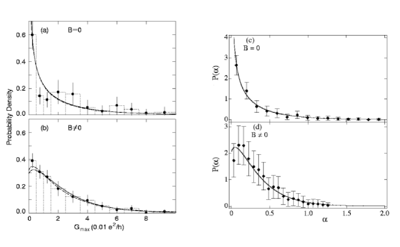
Figure 10: Histograms of conductance peak heights for orthogonal (a,c) and unitary ensembles (b,d). Data (a,b) and (c,d) are taken from [105] and [21] respectively. An example of the raw data used for the graphs (c,d) is shown in Fig. 2 (b).

It is also noteworthy that the average conductance depends on the magnetic field:

$$\langle G_{\rm peak}^{\beta}\rangle=\left(3-2^{3/2}\right)\frac{e^{2}}{\pi\hbar}\left(\frac{\Delta}{T}\right)\frac{\langle g_{1}\rangle\langle g_{2}\rangle}{\left(\langle g_{1}\rangle^{1/2}+\langle g_{2}\rangle^{1/2}\right)^{2}}F\left[2-\beta+\left(\beta-1\right)a\right],$$

(141)

where the asymmetry parameter $a$ was defined in Eq. (140) and the dimensionless function $F(x)$ is given by

$$F(x)=\frac{1+x}{2x}-\frac{(1-x)^{2}}{4x^{3/2}}{\mathrm{a}rcosh}\left(\frac{1+x}{1-x}\right);\quad F(1)=1;\quad F(0)=\frac{4}{3}.$$ (142)

We see from Eqs. (141) and Eq. (142) that the average conductance in the magnetic field (unitary case, $\beta=2$) is larger than in the absence of the field (orthogonal case, $\beta=1$). This phenomenon is analogous to the effect of negative magnetoresistance due to the weak localization in bulk systems [106] with the same physics involved. For the average peak heights, the magnetoresistance is sensitive to the asymmetry of the contacts (140) and in the limiting case of a very asymmetric contacts, $a\to 1$, the magnetoresistance vanishes.

So far, we have presented results for the peak height distributions for ensembles of Coulomb-blockaded quantum dots with either fully preserved or fully broken time-reversal symmetry. To investigate how the crossover between those two ensembles happens for the temperature regime (130), one has to use the statistics of the wavefunctions in the crossover ensemble of random Hamiltonians distributed according to Eq. (2.2). This statistics is described by Eqs. (22) and Eq. (23). To obtain the moments of the conductance at the crossover regime, is a lengthy, albeit straightforward calculation involving Eqs. (132), (136), (22) and (23). We refer the readers to the original papers [100, 107] and review [15] for the results. (The peak height distribution function for the limit $a\to 1$ corresponding to the case of strongly asymmetric contacts was obtained earlier in Ref. [61], see also Ref. [43].

Besides the distribution functions of the peaks heights at a fixed value of the magnetic field, another quantity of interest is the correlation function of the peak heights for different values of the magnetic field. It is defined as

$$C(B_{1},B_{2}) = \frac{\langle\delta G(B_{1})\delta G(B_{2})\rangle}{\left(\langle\delta G(B_{1})^{2}\rangle\langle\delta G(B_{2})^{2}\rangle\right)^{1/2}},$$

$$\delta G(B) = G_{\rm peak}(B)-\langle G_{\rm peak}(B).\rangle$$ (143)

Physically, the correlator $C$ characterizes “how fast” the ensemble changes under the effect of the magnetic field.

The peak-height correlation function (143) was studied numerically in Refs. [101, 102]. For the unitary ensemble, $N_{h}^{C}\gg 1$, the results were found to be well approximated as

$$C(B_{1},B_{2})\approx\frac{1}{\left(1+0.25N_{h}^{D}\right)^{2}},$$ (144)

where the parameters $N_{h}^{D,C}$ are related to the difference and sum of the magnetic fields by Eq. (20). Once again, the characteristic magnetic field is determined by the condition $N_{h}\simeq 1$.

3.2 Mesoscopic fluctuations of Coulomb blockade valleys

In this subsection, we study the mesoscopic fluctuations of the conductance in the regime where the gate voltage ${\cal N}$ is tuned away from the degeneracy point [108], $|{\cal N}-{\cal N}^{\ast}|>T/E_{c}$. Equations (134) and (135) predict in this case the conductance to be exponentially small $G({\cal N})\propto\exp\left[-2E_{c}|{\cal N}-{\cal N}^{\ast}|/T\right]$. However, this expectation is not correct. The rate equations of Sec. 3.1 take into account only processes which are of the first order in the right or left conductance. In these processes a charge is transferred from a lead (initial state) to the dot (final state), or vise versa. In the valleys such processes are exponentially suppressed because of the high energy in the final state. On the other hand, higher order processes allow for both the initial and final states to be in the leads, so that the thermal exponent does not appear. Such processes, commonly referred to as co-tunneling [28], are suppressed only algebraically, $G({\cal N})\propto 1/\left[2E_{c}|{\cal N}-{\cal N}^{\ast}|\right]$, and dominate the transport already at moderate deviations from the conductance peaks.

Such second-order processes are shown in Fig. 11. The processes (a),(b) and (c),(d) are electron-like and hole-like processes, respectively. In an electron-like process, the intermediate state corresponds to an extra electron placed on the dot. In this case the electrostatic part of the energy of the virtual state is given by [see Eq. (92)],

$$E_{e}=2E_{c}\left({\cal N}^{\ast}-{\cal N}\right),$$ (145)

where ${\cal N}^{*}$ is the half-integer corresponding to the Coulomb Blockade peak. For a hole-like process, the intermediate state has one less electron on the dot, so that the electrostatic part of the energy of the virtual state is

$$E_{h}=2E_{c}\left({\cal N}-{\cal N}^{\ast}+1\right).$$ (146)

In writing Eqs. (145) and (146) we consider the dimensionless gate voltages ${\cal N}$ in the interval ${\cal N}^{*}-1<{\cal N}<{\cal N}^{*}$.

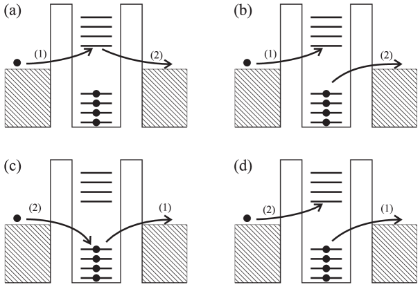
Figure 11: Schematic picture of the second order processes contributing to the conductance in the Coulomb blockade valleys. Processes (a), (b) are electron-like and (c), (d) are hole-like. Elastic co-tunneling [28] corresponds to the processes (a) and (c), and inelastic co-tunneling [27, 28] is described by (b) and (d).

Even though all the processes of Fig. 11 are of the same order in the tunneling constants, there is an important difference between the transitions (a) and (c) on the one hand, and (b) and (d) on the other hand: For the cases (a) and (c), the very same electron (hole) that tunnels into the dot leaves the dot, whereas in the cases (b) and (d), a different electron (hole) tunnels from the dot. The result is that in the cases (b) and (d), the final state differs from the initial state by the excitation of an extra electron-hole pair (inelastic co-tunneling). The phase volume for such a two-particle excitation is proportional to $(\varepsilon_{\rm eh})^{2}$ (if $\varepsilon_{\rm eh}\gg\Delta$), where $\varepsilon_{\rm eh}$ is the energy of the electron-hole pair. Since $\varepsilon_{\rm eh}$ can not exceed the temperature $T$, the inelastic contribution vanishes at low temperature as $T^{2}$, even in the limit $\Delta\to 0$. The elastic contributions (a) and (c), in contrast, are temperature independent. For that reason we here concentrate on the elastic co-tunneling and return to inelastic co-tunneling only at the end of the Section.

The tunneling conductance can be calculated according to the Golden rule as

$$G=2\frac{2\pi e^{2}}{\hbar}\nu^{2}\left|A_{e}+A_{h}\right|^{2},$$ (147)

where $\nu$ is the density of states per one spin in the leads and the extra factor of $2$ takes care of the spin degeneracy. The amplitudes $A_{e}$ and $A_{h}$ correspond to the processes of Fig. 11 (a) and (c), respectively. They can be calculated with the help of the Hamiltonian (97), with Eq. (129) for the matrix $W$, in second order perturbation theory in the tunneling probabilities. The result is

$$A_{e} = \sqrt{\langle g_{1}\rangle\langle g_{2}\rangle}\left(\frac{\Delta M}{4\pi^{2}\nu}\right)\sum_{\alpha}\frac{\psi_{\alpha}(1)\psi_{\alpha}^{\ast}(2)}{\varepsilon_{\alpha}+E_{e}}\theta(\varepsilon_{\alpha});$$

$$A_{h} = -\sqrt{\langle g_{1}\rangle\langle g_{2}\rangle}\left(\frac{\Delta M}{4\pi^{2}\nu}\right)\sum_{\alpha}\frac{\psi_{\alpha}(1)\psi_{\alpha}^{\ast}(2)}{-\varepsilon_{\alpha}+E_{h}}\theta(-\varepsilon_{\alpha}),$$ (148)

where $\varepsilon_{\alpha}$ and $\psi_{\alpha}(i)$ are the exact eigenenergies and eigenvectors of the noninteracting Hamiltonian (13), and the argument $i=1,2$ of the wave function $\psi$ labels the sites coupled to contacts $1$ and $2$, respectively, see Eqs. (129). The eigenenergies $\varepsilon_{\alpha}$ are measured from the upper filled level in the dot, so that step function $\theta(\pm\varepsilon_{\alpha})$ selects empty (occupied) orbital states for electron (hole) like processes of Fig. 11a(c). The relative sign difference in the electron, $A_{e}$, and hole, $A_{h}$, amplitudes comes from the commutation relation of the Fermion operators.

Substituting Eq. (148) into Eq. (147), we find

$$G=\frac{e^{2}}{4\pi^{3}\hbar}\langle g_{2}\rangle\langle g_{1}\rangle|F_{e}+F_{h}|^{2},$$ (149)

where the dimensionless functions $F$ are given by

$$F_{e}=M\Delta\sum_{\alpha}\frac{\psi_{\alpha}(1)\psi_{\alpha}^{\ast}(2)}{\varepsilon_{\alpha}+E_{e}}\theta(\varepsilon_{\alpha});$$

$$F_{h}=M\Delta\sum_{\alpha}\frac{\psi_{\alpha}(1)\psi_{\alpha}^{\ast}(2)}{\varepsilon_{\alpha}-E_{h}}\theta(-\varepsilon_{\alpha}).$$ (150)

It is also possible, and more convenient for some applications, to express $F$ in terms of the exact one electron Green functions of the dot

$$F_{e}=M\Delta\int_{0}^{\infty}\frac{d\varepsilon}{2\pi i}\frac{{\cal G}^{A}_{12}(\varepsilon)-{\cal G}^{R}_{12}(\varepsilon)}{\varepsilon+E_{e}},$$

$$F_{h}=M\Delta\int^{0}_{-\infty}\frac{d\varepsilon}{2\pi i}\frac{{\cal G}^{A}_{12}(\varepsilon)-{\cal G}^{R}_{12}(\varepsilon)}{\varepsilon-E_{h}},$$ (151)

where the Green function is given by Eq. (24).

Equations (149) – (151) solve the part of the problem depending on the interactions; the conductance is expressed in terms of the single electron eigenfunctions and eigenvalues of the isolated dot. What remains is to perform the statistical analysis of the conductance in a fashion similar to what was done in Sec. 3.1 for the peak heights. Note, however, that there is an important difference with the case of the peak height statistics: while the height of a conductance peak depended on the wavefunction of one level only, many levels with energies of the order of $E_{e(h)}$ contribute to the tunneling. The superposition of such a large number of tunneling amplitudes significantly affects the conductance fluctuations [108]. Despite these complications, expressions for the distribution function of the conductance in the regime of elastic co-tunneling, and the correlation function of the conductance in a magnetic field, can be found in closed form. We now describe their calculation.

The cases of the pure orthogonal ($\beta=1$) or unitary ensembles ($\beta=2$) are the easiest to investigate. We use the fact that the eigenvectors and eigenvalues of a random matrix in these cases are independent of each other. Moreover, the eigenvectors of different eigenstates are also Gaussian variables independent of each other, see Eq. (21).

Using Eq. (150) and Eq. (21), we immediately find

$$\langle F_{e}\vphantom{o}F_{e}^{\ast}\rangle=\Delta^{2}\sum_{\alpha}\theta(\varepsilon_{\alpha}){\left\langle\frac{1}{\left(\varepsilon_{\alpha}+E_{e}\right)^{2}}\right\rangle}.$$ (152)

Since the averaged density of states does not depend on energy, and since we consider $E_{e},E_{h}\gg\Delta$, we can replace the summation $\Delta\sum_{\alpha}$ by the integration $\int d\varepsilon_{\alpha}$ in Eq. (152). The resulting expressions are

$$\langle F_{e}F_{e}^{\ast}\rangle=\frac{\Delta}{E_{e}},\quad\langle F_{e}F_{e}\rangle=\left(\frac{2}{\beta}-1\right)\frac{\Delta}{E_{e}};$$

$$\langle F_{h}F_{h}^{\ast}\rangle=\frac{\Delta}{E_{h}},\quad\langle F_{h}F_{h}\rangle=\left(\frac{2}{\beta}-1\right)\frac{\Delta}{E_{h}};$$

$$\langle F_{e}F_{h}^{\ast}\rangle=\langle F_{e}F_{h}\rangle=0,$$ (153)

where all the averages are found in the same fashion as (152).

Using Eq. (153), we can find the average of the conductance (149):

$$\langle G\rangle=\frac{e^{2}}{4\pi^{3}\hbar}\langle g_{2}\rangle\langle g_{1}\rangle\left[\frac{\Delta}{E_{e}}+\frac{\Delta}{E_{h}}\right].$$ (154)

This expression was first obtained in [28] by a different method of the ensemble averaging. (To calculate the quantitites of the type of Eq. (153), the authors of Ref. [28] used the technique developed in the semiclassical theory of inhomogeneous superconductors [109, 110].) Notice that a magnetic field has no effect on the average conductance; $\langle G\rangle$ remains the same for the unitary and orthogonal ensembles. We remind the reader that Eq. (154) is obtained within the RMT theory, and therefore assumes $E_{c}\ll E_{T}$.

However, as we show below, the fluctuations of the conductance are of the order of the average conductance, so that the average (154) is not a good representative of the ensemble. In order to characterize the conductance fluctuations, we need higher moments of the factors $F_{e}$ and $F_{h}$ than those calculated in Eq. (150). Using Eq. (21), we find

$$\langle(F_{e}F_{e}^{\ast})^{2}\rangle=\left(4-\beta\right)\Delta^{4}\sum_{\alpha,\gamma}\theta(\varepsilon_{\alpha})\theta(\varepsilon_{\gamma})\left\langle\frac{1}{\left(\varepsilon_{\alpha}+E_{e}\right)^{2}}\frac{1}{\left(\varepsilon_{\gamma}+E_{e}\right)^{2}}\right\rangle.$$ (155)

Further simplification follows from the condition $E_{e}\gg\Delta$. It enables us to neglect the level repulsion and substitute $\Delta^{2}\sum_{\alpha,\gamma}\to\int d\varepsilon_{\alpha}d\varepsilon_{\gamma}$. One easily checks that the corrections to this approximation are of the order of $(\Delta/E_{e})^{2}\ln(E_{e}/\Delta)\ll 1$. As a result, we have

$$\langle(F_{e}F_{e}^{\ast})^{2}\rangle=2\langle F_{e}F_{e}^{\ast}\rangle^{2}+\langle F_{e}^{\ast}F_{e}^{\ast}\rangle\langle F_{e}F_{e}\rangle,$$ (156)

where the irreducible averages are given in Eq. (153). Equation (156) indicates that the amplitudes $F$ entering the conductance are random Gaussian variables with zero average and variance (153). (This can be proven by explicit consideration of the higher moments.) This observation immediately allows one to compute the fluctuations of the conductance in the valley,

$$\frac{\langle\delta G^{2}\rangle}{\langle G\rangle^{2}}=\frac{2}{\beta}.$$ (157)

With the breaking of time reversal symmetry the fluctuations are reduced by a factor of $2$ similar to the conductance fluctuations in the bulk systems, $\langle G\rangle\gg e^{2}/(\pi\hbar)$. For the cases of $E_{e}\gg E_{h}$ or $E_{e}\ll E_{h}$ (vicinity to the Coulomb blockade peak), Eq. (157) was first obtained in [108].

It is clear from Eq. (157) that the fluctuations of the conductance are of the order of the conductance itself, despite the naive expectation that the large number of the contributing states produce the self-averaging. The reason for this, is that we have to add amplitudes, not probabilities, to compute the conductance.

Because the fluctuations of the conductance are large, its distribution function is not Gaussian. However, it can be found analytically with the help of Eq. (149) and the established fact that $F$’s are Gaussian variables with the variances (153). Straightforward calculation yields that the distribution of $G$ normalized to its average is given by

$$W(\alpha)=\left\langle\delta\left(\alpha-\frac{G}{\langle G\rangle}\right)\right\rangle=\cases{\theta(\alpha)\displaystyle{\frac{e^{-\alpha/2}}{\sqrt{2\pi\alpha}}};&$\beta=1$\cr\theta(\alpha){e^{-\alpha}}&$\beta=2$},$$ (158)

which coincides with Porter-Thomas distribution [59]. This was to be expected from the central limit theorem, because the conductance is determined by a large number of random amplitudes, which is exactly the assumption behind the Porter-Thomas distribution.

Now, we turn to the study of the effect of the magnetic field on the valley conductance. Our purpose is to find the correlation function for the conductance fluctuations, similar to Eq. (143), and the distribution function on the crossover between orthogonal and the unitary ensembles. Here we discuss only the situation in the vicinity of the peaks, which corresponds to the condition $E_{e}\gg E_{h}$ or $E_{e}\ll E_{h}$, so that only one contribution is dominant. The results for the general case are presented in Appendix D. Because a large number of levels contribute to the transport of electrons through the quantum dot, we can use Eq. (151) and then apply Eq. (25) to average the product of the Green functions. We thus find that the amplitudes $F$ are still Gaussian variables, while their averages are modified in comparison with Eq. (153):

$$\langle F_{e}F_{e}^{\ast}\rangle=\frac{\Delta}{E_{e}}{\Lambda\left(\frac{N_{h}^{D}\Delta}{2\pi E_{e}}\right)},\quad\langle F_{e}F_{e}\rangle=\frac{\Delta}{E_{e}}{\Lambda\left(\frac{N_{h}^{C}\Delta}{2\pi E_{e}}\right)};$$ (159)

$$\langle F_{h}F_{h}^{\ast}\rangle=\frac{\Delta}{E_{h}}{\Lambda\left(\frac{N_{h}^{D}\Delta}{2\pi E_{h}}\right)},\quad\langle F_{h}F_{h}\rangle=\frac{\Delta}{E_{h}}{\Lambda\left(\frac{N_{h}^{C}\Delta}{2\pi E_{h}}\right)}.$$ (160)

Here the dimensionless function $\Lambda(x)$ is given by

$$\Lambda(x) = \frac{1}{\pi x}\left[\ln x\ln(1+x^{2})+\pi\arctan x+\frac{1}{2}{\mathrm{L}i}_{2}(-x^{2})\right],$$ (161)

with ${\mathrm{L}i}_{2}(x)$ being the second polylogarithm function [103]. The asymptotic behavior of function $\Lambda$ is $\Lambda(x)=1+(x\ln x)/\pi$, for $x\ll 1$, and $\Lambda(x)=(\pi x)^{-1}\ln^{2}x$, for $x\gg 1$. The parameters $N_{h}^{D}$ and $N_{h}^{C}$ are defined in Section 2.2. The limits of the pure orthogonal (unitary) ensembles (153) are recovered by putting $N_{h}^{D}=0$ and $N_{h}^{C}=0(\infty)$ in Eq. (159).

The correlation function acquires a universal form [108] (i.e., all the dependences for different $E_{e(h)}$ can be collapsed to a single curve upon rescaling of the magnetic field):

$$C(B_{1},B_{2}) = \frac{\langle\delta G(B_{1})\delta G(B_{2})\rangle}{\langle G\rangle^{2}}$$ (162)

$$= \left\{\Lambda\left[\left(\frac{\Phi_{1}+\Phi_{2}}{\Phi_{c}}\right)^{2}\right]\right\}^{2}+\left\{\Lambda\left[\left(\frac{\Phi_{1}-\Phi_{2}}{\Phi_{c}}\right)^{2}\right]\right\}^{2},$$

where the scaling function $\Lambda(x)$ is defined in Eq. (161), $\Phi_{i}$ is the magnetic flux through the dot due to the field $B_{i}$, and the correlation magnetic flux $\Phi_{c}$ is controlled by the charging energy

$$\Phi_{c}=\frac{1}{\sqrt{\chi g}}\left(\frac{2\pi E}{\Delta}\right)^{1/2}\Phi_{0},\quad E={\mathrm{m}in}\left(E_{e},\ E_{h}\right),$$ (163)

where $\Phi_{0}$ is the flux quantum, $g$ is the dimensionless conductance of the closed dot, see Sec. 2, and the dimensionless coefficient $\chi$ is discussed after Eq. (20). The dependence of the correlation flux on the charging energy is caused by the fact that the transport is contributed to by a large number of states in the energy strip of the order of $E$ (see the discussion in Sec. 2.2), which depends on the gate voltage.

We emphasize that the functional form of $C(\Delta B)$ is different from the results for the peak heights fluctuations (144), see Fig. 12. It is worth noticing from Eq. (154) and Eq. (163) that in this regime, the correlation magnetic flux $\Phi_{c}$ drops with approaching a charge degeneracy point, whereas the quantity $\langle G\rangle\Phi_{c}^{2}$ remains invariant.

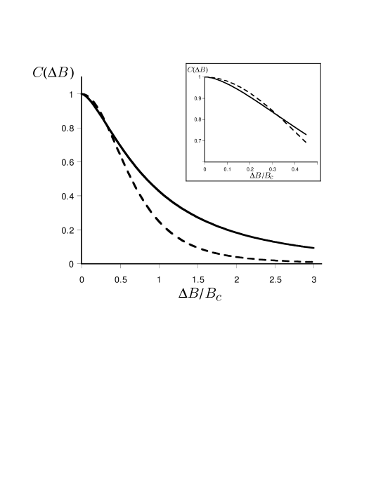
Figure 12: The correlation function $C(\Delta B=B_{1}-B_{2})$ for the conductance fluctuations in the elastic co-tunneling regime (solid line) and for the peak height fluctuations $C=[1+(\Delta B/B_{c})^{2}]^{-2}$ (dashed line) in the regime $\Phi_{1},\Phi_{2}\gg\Phi_{c}$. For the elastic co-tunneling, $C(\Delta B)$ is non-analytic at $\Delta B\to 0$, see the inset, and Eq. (162).

The distribution function of the conductance in the crossover regime can be found from Eq. (149) and the fact that the amplitudes $F$ are Gaussian with the correlators (159). The calculation yields, instead of (158), a distribution function characterized by a single crossover parameter $\lambda$,

$$W(\alpha)=\frac{\theta(\alpha)}{\sqrt{1-\lambda^{2}}}\exp\left(-\frac{\alpha}{1-\lambda^{2}}\right){\mathrm{I}}_{0}\left(\frac{\alpha\lambda}{1-\lambda^{2}}\right);$$ (164)

here ${\mathrm{I}}_{0}(x)$ is the zeroth order modified Bessel function of the first kind. In the limiting cases $\lambda=1$ and $\lambda=0$, the distribution function $P(g)$ coincides with the Porter-Thomas distribution (158) for the orthogonal and unitary ensembles respectively.

The dependence of the crossover parameter $\lambda$ on the magnetic flux $\Phi$ in our case is quite nontrivial [108]

$$\lambda=\Lambda\left(\frac{4\Phi^{2}}{\Phi_{c}^{2}}\right),$$ (165)

where the correlation flux is given by Eq. (163), and function $\Lambda(x)$ is defined in Eq. (161). The crossover in the mesoscopic fluctuations of conductance in the valleys far from the peaks is discussed in Appendix D.

The interference effects in the Coulomb blockade valleys were studied experimentally in Ref. [111]. In agreement with the theory of this section it was found that the average conductance does not show a weak localization correction (it remains the same for the unitary and orthogonal ensembles). The statistics of mesoscopic fluctuations of the valley conductance also agrees reasonably well with the theory. Extracted with the help of Eq. (162), the dependence of the correlation magnetic field on the gate voltage across a valley is shown in Fig. 13. One can see that the correlation magnetic field increases with the deviation from a conductance peak, in agreement with Eq. (163). However, the value of the ratio of the correlation fields for peaks, see Sec. 3.1, and for the valleys was found somewhat smaller than the theoretical prediction.

Figure 13: Ensemble-averaged characteristic correlation field (solid) and average conductance (dashed) across peak-valley-peak for $\sim 14$ independent data sets.

We recall that a relatively large correlation magnetic field in a valley results from a wide energy band ($\sim E_{c}/\Delta$) of virtual discrete states in the dot. By the same token, the conductance in adjacent valleys is also correlated, because all but one virtual states participating in transport are the same for such valleys. In fact the conductance remains correlated over a large number $\sim E_{c}/\Delta$ of valleys. The corresponding corellation function was calculated in Ref. [112], and the valley-valley correlation function for the differential capacitances was found in Ref. [113].

Considering electron transport through a blockaded dot, we have used so far finite-order perturbation theory in the dot-lead tunneling amplitudes. If the dot carries a non-zero spin, like in the case of an odd number of electrons on the dot, such a treatment may miss specific effects caused by the degeneracy of the spin state of an isolated dot. Tunneling results in the exchange interaction between the spins of the dot and leads. The exchange, in turn, leads to a many-body phenomenon, the Kondo effect. This effect results in an unexpected temperature dependence of the conductance across the dot at temperatures $T\ll\Delta$.

3.3 Kondo effect in a strongly blockaded dot

The Kondo effect is one of the most studied and best understood problems of many-body physics. Initially, the theory was developed to explain the increase of resistivity of a bulk metal with magnetic impurities at low temperatures [114]. Soon it was realized that Kondo’s mechanism works not only for electron scattering, but also for tunneling through barriers with magnetic impurities [115, 116, 117]. A non-perturbative theory of the Kondo effect has predicted that the cross-section of scattering off a magnetic impurity in the bulk reaches the unitary limit at zero temperature [118]. Similarly, the tunneling cross-section should approach the unitary limit at low temperature and bias [119, 120] in the Kondo regime.

The Kondo problem can be discussed in the framework of Anderson’s impurity model [121]. The three parameters defining this model are: the on-site electron repulsion energy $U$, the one-electron on-site energy $\varepsilon_{0}$, and the level width $\Gamma$ formed by hybridization of the discrete level with the states in the bulk. The non-trivial behavior of the conductance occurs if the level is singly occupied, $\Gamma<|\varepsilon_{0}|<U$, and the temperature $T$ is below the Kondo temperature

$$T_{K}\simeq\sqrt{U\Gamma}\exp\left\{\frac{\pi\varepsilon_{0}(\varepsilon_{0}+U)}{2\Gamma U}\right\},$$ (166)

where $\varepsilon_{0}<0$ is measured from the Fermi level [122].

Before considering the Kondo effect in a quantum dot, we first review it for tunneling through a single localized level with on-site repulsion $U$ using the Hamiltonian of the Anderson model,

$${\hat{H}}_{A} = \sum_{q,\sigma}\xi_{q}(a_{1q\sigma}^{\dagger}a_{1q\sigma}+a_{2q\sigma}^{\dagger}a_{2q\sigma})+\sum_{\sigma}\varepsilon_{0}a_{0\sigma}^{\dagger}a_{0\sigma}+U{\hat{n}}_{\uparrow}{\hat{n}}_{\downarrow}$$ (168)

$$\mbox{}+\sum_{q,\sigma}(t_{1}a_{1q\sigma}^{\dagger}+t_{2}a_{2q\sigma}^{\dagger})a_{0\sigma}+a_{0\sigma}^{\dagger}(t_{1}a_{1q\sigma}+t_{2}a_{2q\sigma}),$$

$${\hat{n}}_{\sigma} = a_{0\sigma}^{\dagger}a_{0\sigma}.$$

Here $a_{1q\sigma}^{\dagger}$, $a_{2q\sigma}^{\dagger}$, and $a_{0\sigma}^{\dagger}$ are the electron creation operators in the left and right leads ($1$ and $2$), and on the localized level, respectively; $\xi_{q}$ are the corresponding energies in the electron continuum. For brevity, the tunneling matrix elements $t_{1}$ and $t_{2}$ connecting the localized state in the dot with the states in the leads are taken to be $q$-independent. The widths $\Gamma_{i}$ are related to these tunneling matrix elements: $\Gamma_{i}=2\pi\nu_{i}|t_{i}|^{2}$, where $\nu_{i}$ is the density of states of lead $i=1,2$. At first sight, an Anderson impurity in a two-band model (168) may be associated with a two-channel Kondo problem [123]. However, it is easy to show that in our case the parameters of this two-channel problem are such that it can be reduced to the conventional single-channel one. Indeed, by a unitary transformation

$$\left\{\begin{array}[]{l}\alpha_{q\sigma}\\ \beta_{q\sigma}\end{array}\right\}=ua_{1q\sigma}\pm va_{2q\sigma},\;\mbox{with}\quad\left\{\begin{array}[]{l}u\\ v\end{array}\right\}=\frac{1}{\sqrt{|t_{1}|^{2}+|t_{2}|^{2}}}\left\{\begin{array}[]{l}t_{1}\\ t_{2}\end{array}\right\},$$ (169)

The Hamiltonian (168) can be converted [120] to the conventional one-band model with Anderson impurity [121]. The localized state and band described by the fermion operators $\alpha_{q\sigma}$ form the usual Anderson impurity model, which is characterized by three parameters: $U$, $\varepsilon_{0}$, and $\Gamma=\Gamma_{1}+\Gamma_{2}$. The band described by the operators $\beta_{q\sigma}$ is entirely decoupled from the impurity. The scattering amplitude ${\cal A}(1,q\to 2,q^{\prime})$ between two states in the opposite leads is related to the scattering amplitudes ${\cal A}(\alpha,q\to\alpha,q^{\prime})$ and ${\cal A}(\beta,q\to\beta,q^{\prime})$ within the bands $\alpha$ and $\beta$, respectively, by relation

$${\cal A}(1,q\to 2,q^{\prime})=uv[{\cal A}(\alpha,q\to\alpha,q^{\prime})-{\cal A}(\beta,q\to\beta,q^{\prime})].$$

The scattering amplitude in the $\alpha$–band is directly related to the scattering phase $\delta_{K}$ for the conventional Kondo problem, ${\cal A}(\alpha,q\to\alpha,q)=\exp(2i\delta_{K})$; the scattering problem for the $\beta$–band is trivial, ${\cal A}(\beta,q\to\beta,q)=1$. Using Eq. (169), we finally find

$$|{\cal A}(1,q\to 2,q)|^{2}=4|uv|^{2}\sin^{2}\delta_{K}=\frac{4g_{1}g_{2}}{(g_{1}+g_{2})^{2}}\sin^{2}\delta_{K}.$$

This way, the “Kondo conductance” $G_{K}$ associated with the spin-degenerate localized level can be expressed in terms of the problem of one-channel scattering off a single Kondo impurity in a bulk material,

$$G_{K}=\frac{e^{2}}{\pi\hbar}\frac{4g_{1}g_{2}}{(g_{1}+g_{2})^{2}}f\left(\frac{T}{T_{K}}\right).$$ (170)

Here $T_{K}$ is the characteristic Kondo temperature, and $f(x)$ is a universal function. This function, found with the help of numerical renormalization group in Ref. [125], is plotted in Fig. 14. A remarkable property of scattering on a Kondo impurity, is that the corresponding cross-section approaches the unitary limit at low energies, $f(0)=1$. The low-temperature correction to the unitary limit is proportional to $T^{2}$ and described by Nozières’ Fermi-liquid theory [118],

$$f\left(\frac{T}{T_{K}}\right)=1-\frac{\pi^{2}T^{2}}{T_{K}^{2}},\quad T\ll T_{K}.$$ (171)

So far we considered the Kondo-enhanced tunneling through a single level. The same situation can be realized in tunneling through a quantum dot. The number of electrons in the dot is controlled by the applied gate voltage. If this number is an odd integer, $2n+1$, i.e., the dimensionless gate voltage ${\cal N}=C_{g}V_{g}/e$ lies in the interval

$$|{\cal N}-(2n+1)|<\frac{1}{2},$$ (172)

the Kondo effect leads to a dramatic increase of the conductance at low temperatures. The consequence is an even-odd alternation of the valley conductance through the quantum dot: In “even” valleys, the low temperature conductance is due to elastic co-tunneling, while in “odd” valleys, the presence of an unpaired spin in the highest occupied level leads to the Kondo effect, which causes a remarkable increase of the low temperature conductance compared to the even valleys.

Figure 14: Plot of the universal function $y=f(x)$ vs. $x=T/T_{K}$ from Ref. ([125]).

The advantage of using the quantum dots for the experimental studies of the Kondo effect stems from an opportunity to effectively control the parameters of the system, which is hardly possible for a magnetic impurity embedded in a host material.

Quantitatively, the low-temperature limit for the conductance in the odd valleys is given by Eqs. (170) and (171). The Kondo temperature $T_{K}$, Eq. (166)) depends on the gate voltage through parameter $\varepsilon_{0}$:

$$\varepsilon_{0}=2E_{c}({\cal N}-{\cal N}^{*})<0,\quad U=2E_{c},$$ (173)

where ${\cal N}^{*}=n+\frac{1}{2}$ is the degeneracy point at which two different charge states of the dot have the same energy.

At a first glance, it appears that the Kondo temperature for a quantum dot may be obtained by the substitution of the parameters Eq. (173) into Eq. (166). However, it is not exactly the case, as we explain below. Unlike the single-level Anderson impurity model, the discrete energy spectrum of a dot is dense, $\Delta\ll E_{c}$. Still, if the junctions’ conductances are small, $G_{i}\ll e^{2}/\hbar$, (strong Coulomb blockade), those levels of the dot which are doubly-filled or empty are important only at scales larger than one-electron level spacing, and only the one single-occupied level contributes to the dynamics of the system at energy scale smaller than $\Delta$. As a result, the model of the dot attached to two leads can be truncated to the Anderson impurity model, however the high energy cut-off is determined by $\Delta$ rather than by the charging energy. (See Sec. 4.3 for more discussions). This change in the energy cut-off replaces the first factor $U$ in Eq. (166) by $\Delta$. The level width $\Gamma$ can be related to the sum $g_{1}+g_{2}$ for a given level in the quantum dot. Finally, Eq. (173) establishes the relation between $\varepsilon_{0}$ and $U$ on the one hand, and the charging energy $E_{c}$ and gate voltage ${\cal N}$ on the other hand. The resulting Kondo temperature (for the interval $0<{\cal N}-{\cal N}^{*}\simeq 1/2$) is found as

$$T_{K}\simeq\Delta\sqrt{(g_{1}+g_{2})\frac{\Delta}{E_{c}}}\exp\left[-\frac{2\pi}{g_{1}+g_{2}}\frac{E_{c}}{\Delta}({\cal N}-{\cal N}^{*})\right].$$ (174)

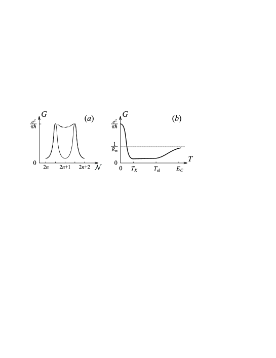
Figure 15: (a) Linear conductance at $T\gg T_{K}$ (solid line) and $T\>{{}^{{}_{\displaystyle<}}_{\displaystyle\sim}}\>T_{K}$ (dotted line). Due to the Kondo effect, the function $G({\cal N})$ develops plateaux in place of the “odd” valleys of the Coulomb blockade. (b) Sketch of the temperature dependence of the linear conductance, $G(T)$, in the “odd” valley. The conductance decreases with the decrease of temperature from $T\sim E_{c}$ down to $T\sim T_{\rm el}\simeq\sqrt{E_{c}\Delta}$, see, e.g., [28, 108], and Eq. (183). At very low temperatures, $T\>{{}^{{}_{\displaystyle<}}_{\displaystyle\sim}}\>T_{K}$, the conductance grows again. If the singly-occupied level, which gives rise to the Kondo effect, has equal partial widths, $\Gamma_{1}=\Gamma_{2}$, the conductance reaches the unitary limit $G=e^{2}/\pi\hbar$ at low temperatures.

Equations (170) and (171) tell us that upon sufficiently deep cooling, the gate voltage dependence of the conductance through a quantum dot should exhibit a drastic change. Instead of the “odd” valleys, which correspond to the intervals of gate voltage (172), plateaux in the function $G({\cal N})$ develop, see Fig. 15a. In other words, the temperature dependence of the conductance in the “odd” valleys should be very different from the one in the “even” valleys. The conductance, determined by the activation and inelastic co-tunneling mechanisms, decreases monotonously with the decrease of temperature, and then saturates at the value of $G_{\rm el}$ in the even valleys, see the previous Section. On the contrary, if the gate voltage is tuned to one of the intervals (172), the $G(T)$ dependence is non-monotonous, see Fig. 15b. When temperature is lowered, the conductance first drops due to the Coulomb blockade phenomenon. A further decrease of temperature results in the increase of the conductance at $T\>{{}^{{}_{\displaystyle<}}_{\displaystyle\sim}}\>T_{K}$. Its $T=0$ saturation value depends on the ratio of the partial level widths $\Gamma_{1}$ and $\Gamma_{2}$ of a particular discrete level. The partial widths are related to the tunneling matrix elements, $\Gamma_{i}=2\pi\nu|t_{i}|^{2}\propto g_{i}$, where the matrix elements $t_{i}$, in turn, are proportional to the values of the electron eigenfunctions within the dot, $t_{i}\propto\psi_{n}(i)$, where $n$ labels the eigenstate, and the argument $i$ of the wavefunction $\psi_{n}$ refers to the site in the dot adjacent to junction $i$, see Eqs. (128) and (132). In a disordered or chaotic dot, the electron wave functions are random quantities, described by the Porter-Thomas distribution [59]. As we already discussed in the previous section the randomness of the wave functions results in mesoscopic fluctuations of the elastic co-tunneling conductance [108]. The $T=0$ value of the conductance in the Kondo regime should fluctuate as well, see Eq. (170). Experiments are performed, however, at a finite temperature $T$, where fluctuations of conductance occur mostly due to the fluctuation of the Kondo temperature (174), which has an exponential dependence on the level width $\Gamma_{1}+\Gamma_{2}$.

The experimental search for a tunable Kondo effect brought positive results [126, 127, 128] only recently. In a number of experiments the difference in the low-temperature conductance behavior in the “odd” and “even” valleys was clearly observed, see Fig. 16. In retrospect it is clear, why such experiments were hard to perform. The negative exponent in Eq. (174) contains a product of two large parameters, $E_{c}/\Delta$ and $e^{2}/h(G_{1}+G_{2})$, leading to a very small value of $T_{K}$.

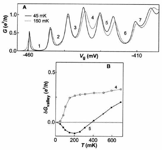
Figure 16: The gate voltage dependence of the conductance at various temperatures (A), and the temperature dependence of the conductance in the valleys labelled 4 and 5 (B), see [127]. Reprinted with permission from Science 281, 540 (1998). Copyright 1998 American Association for the Advancement of Science.

To bring $T_{K}$ within the reach of a modern low-temperature experiment, one may try smaller quantum dots in order to decrease $E_{c}/\Delta$; this route obviously has technological limitations. (In the experiments [126] this ratio was $E_{c}/\Delta\>{{}^{{}_{\displaystyle>}}_{\displaystyle\sim}}\>7$.) Another, complementary option is to increase the junction conductances, so that $G_{1,2}$ come close to $e^{2}/\pi\hbar$, which is the maximal conductance of a single-mode quantum point contact. The junctions in the experiments [126] were tuned to $G\simeq(0.3-0.5)e^{2}/\pi\hbar$. Under these conditions, one would expect $T_{K}\>{{}^{{}_{\displaystyle>}}_{\displaystyle\sim}}\>100$mK only if ${\cal N}-{\cal N}^{*}\>{{}^{{}_{\displaystyle<}}_{\displaystyle\sim}}\>0.07$, see Eq. (174); in the middle of the valley (${\cal N}-{\cal N}^{*}=0.5$) the Kondo temperature is unobservably small. Indeed, an evidence for the Kondo effect was found [126] in a relatively narrow interval interval, ${\cal N}-{\cal N}^{*}\>{{}^{{}_{\displaystyle<}}_{\displaystyle\sim}}\>0.15$. Only in this domain of gate voltages the anomalous increase of conductance $G(T)$ with lowering the temperature $T$ was clearly observed; the anomalous temperature dependence of the conductance was not seen in the middle of the Coulomb blockade valley.

In conventional Kondo systems, a signature of the effect is in the characteristic minimum of the resistivity. The minimum comes from the competition of the two contributions to the resistivity: the phonon contribution is decreasing with lowering the temperature, while the Kondo contribution has the opposite temperature dependence. A similar feature in tunneling through a quantum dot would be a minimum in the conductance in an “odd” valley. However, such a minimum is quite shallow at $G_{1},G_{2}\ll e^{2}/\hbar$. Indeed, the minimum comes from the competition of the temperature dependencies of the inelastic co-tunneling and of the Kondo contribution. In the domain $T\ll\Delta$ the inelastic contribution to the co-tunneling is exponentially small, $G_{\rm in}\propto\exp(-\Delta/T)$. The proper expansion of the function $f(T/T_{K})$ in Eq. (170) at $T\gg T_{K}$ and the use of (174) yield the following temperature dependence of the Kondo contribution to the valley conductance

$$\langle G(T)\rangle=\langle G_{\rm el}\rangle\left[1+\frac{\hbar(G_{1}+G_{2})}{e^{2}}\left(\frac{\Delta}{E_{c}}\right)^{2}\ln\left(\frac{\Delta}{T}\right)+\dots\right],$$ (175)

where $\langle G_{\rm el}\rangle=(\hbar\langle G_{1}\rangle\langle G_{2}\rangle/{4\pi e^{2}})({\Delta}/{E_{c}})$ is the average elastic co-tunneling conductance, see Eq. (154). As one can see from Eq. (175), the Kondo correction to the conductance remains particularly small everywhere in the temperature region $T\>{{}^{{}_{\displaystyle>}}_{\displaystyle\sim}}\>T_{K}$.

In order to increase the Kondo temperature and to observe the anomaly of the temperature-dependent conductance $G(T)$ under these unfavorable conditions, one may try to make the junction conductances larger. However, if $G_{1,2}$ come close to $e^{2}/\pi\hbar$, the discreteness of the number of electrons on the dot is almost completely washed out [39]. Exercising this option, therefore, raises a question about the nature of the Kondo effect in the absence of strong charge quantization. We address this question later on, in Section 4.3.

3.4 Overall temperature and gate voltage dependence of the conductance

Closing this Section, we briefly discuss the gate voltage dependence of the linear conductance through a strongly blockaded dot in various temperature intervals.

As we have already mentioned in the very beginning of Subsection 3.2, rate equations predict that the peaks in the $G({\cal N})$ function should have width $\sim T/E_{c}$; the conductance in the valleys is exponentially small, with the activation energy set by the charging effect. In the temperature interval $E_{c}\gg T\gg\Delta$, the rate equations yield [129] for the peak shape

$$G({\cal N},T)=\frac{e^{2}}{2\pi\hbar}\bar{g}\frac{E_{c}({\cal N}-{\cal N}^{*})/T}{\sinh[E_{c}({\cal N}-{\cal N}^{*})/T]},$$ (176)

where ${\cal N}^{*}$ is a half-integer number, and the parameter $\bar{g}$ is determined by the conductances of the point contacts $\langle g_{1,2}\rangle$, the statistical properties of the wave-functions of the dot, and by the rate of inelastic processes.

If the rate of inelastic processes $1/\tau_{\varphi}$ is small compared to the inverse electron dwell time in the dot $\left(g_{1}+g_{2}\right)\Delta$, then the parameter $\bar{g}$ is given by

$$\bar{g}=\left\langle\frac{g_{1}g_{2}}{g_{1}+g_{2}}\right\rangle=\frac{\langle g_{1}\rangle\langle g_{2}\rangle}{\left(\langle g_{1}\rangle^{1/2}+\langle g_{2}\rangle^{1/2}\right)^{2}}F\left[2-\beta+\left(\beta-1\right)a\right].$$ (177)

Here, $\beta=1,2$ in the limits of no and strong magnetic fields respectively; the parameter of asymmetry of the point contacts $a$ and the function $F$ are defined in Eqs. (140) and (141). The conductance (176) has the same dependence on magnetic field as the averaged peak conductance in the low-temperature ($T\ll\Delta$) regime, see Eq. (141). Notice, that unlike the low-temperature peak conductance, the mesoscopic fluctuations on top of result (176) are suppressed by a large factor of $\Delta/T$ due to the large number of discrete levels contributing to the transport; all the peaks have the same height, which equals the half of the high-temperature ($T\gg E_{c}$) value of conductance through the dot. This is a very straightforward consequence of the Coulomb blockade: out of the two elementary processes of charge transfer (one is increasing, and another is decreasing the initial charge of the dot by $e$), only one process is allowed.

The important difference between the case of sequential tunneling through the quantum dot mentioned above and the process of elastic co-tunneling considered in Section 3.2, is that for sequential tunneling each level contributes to a real process, rather than serves as a virtual state for tunneling as is the case for elastic cotunneling. Therefore, for sequential tunneling not amplitudes, but the probabilities of tunneling through each level are added.

In the case of rapid inelastic relaxation, $1/\tau_{\varphi}\gg\left(g_{1}+g_{2}\right)\Delta$, the time elapsing between the events of an electron tunneling into and out of the dot is sufficiently long that an equilibrium electron distribution can be established inside the dot. If, in addition, the temperature $T\gg\Delta$, an electron entering the dot uses one of many ($\sim\Delta/T$) discrete levels in it. Similarly, an equally large number of levels participates when the electron exits the dot. Because the energy level used for the tunneling from the dot is most probably different from the one used for the tunneling into the dot, the dimensionless conductances $g_{1}$ and $g_{2}$ defined in Eq. (132), has to be independently averaged over many levels, yielding

$$\bar{g}=\frac{\langle g_{1}\rangle\langle g_{2}\rangle}{\langle g_{1}\rangle+\langle g_{2}\rangle}.$$ (178)

The two cases of rapid and slow inelastic relaxation can be distinguished through their magnetoconductance, which, if normalized by the average peak height, is temperature independent as long as inelastic processes are not slow, $1/\tau_{\varphi}\ll(g_{1}+g_{2})\Delta$, but quickly disappears for $T\>{{}^{{}_{\displaystyle>}}_{\displaystyle\sim}}\>\Delta$ when $1/\tau_{\varphi}\gg(g_{1}+g_{2})\Delta$ [130]. Recent measurements of the magnetoconductance of Coulomb blockade peak heights show values between the two extremes of rapid and slow inelastic relaxation [131].

At lower temperatures $T\ll\Delta$, the peaks heights are proportional to $1/T$, and exhibit strong mesoscopic fluctuations, see Subsection 3.1. The peak height reaches

$$G_{\rm peak}\sim\frac{e^{2}}{\pi\hbar}\frac{g_{1}g_{2}}{(g_{1}+g_{2})^{2}},$$ (179)

when $T$ becomes of the order of the discrete level width $(g_{1}+g_{2})\Delta$. At the same time the dimensionless peak width $\delta{\cal N}_{\rm peak}$ decreases down to the value

$$\delta{\cal N}_{\rm peak}\sim(g_{1}+g_{2})\frac{\Delta}{E_{c}}.$$ (180)

When the temperature is further lowered, the peak continues to grow, and simultaneously broadens again and becomes asymmetric. However,these effects become noticeable at much lower temperature, $T\sim T_{K}$, when the Kondo effect starts playing role.

In the valleys, upon lowering the temperature, the exponential decrease of the conductance that was mentioned above is replaced by a weaker, power-law ($\propto T^{2}$) temperature dependence provided by the mechanism of inelastic co-tunneling [27, 28]. In the middle of the valley this mechanism results in the conductance

$$G_{\rm in}=\frac{4}{3\pi}\frac{e^{2}}{\hbar}\langle g_{1}\rangle\langle g_{2}\rangle\left(\frac{T}{E_{c}}\right)^{2}.$$ (181)

One can see that the crossover between the two regimes occurs at temperatures

$$T\simeq T_{\rm in}\equiv E_{c}/|\ln(\langle g_{1}\rangle+\langle g_{2}\rangle)|.$$ (182)

A comparison of Eq. (182) with the result (154) for elastic co-tunneling shows that the crossover to the temperature-independent conductance occurs at

$$T\simeq T_{\rm el}\equiv\sqrt{E_{c}\Delta}.$$ (183)

If the dot carries a finite spin, then at much lower temperatures, $T\>{{}^{{}_{\displaystyle<}}_{\displaystyle\sim}}\>T_{K}$, the conductance increases again due to the Kondo effect, see Subsection 3.3 and Fig 15.

In a typical experiment with a quantum dot formed in a semiconductor heterostructure, the five relevant energy scales are related as:

$$T_{K}\>{{}^{{}_{\displaystyle<}}_{\displaystyle\sim}}\>\Delta\>{{}^{{}_{\displaystyle<}}_{\displaystyle\sim}}\>T_{\rm el}\>{{}^{{}_{\displaystyle<}}_{\displaystyle\sim}}\>T_{\rm in}\>{{}^{{}_{\displaystyle<}}_{\displaystyle\sim}}\>E_{c}.$$ (184)

Temperatures $T\>{{}^{{}_{\displaystyle<}}_{\displaystyle\sim}}\>T_{\rm el}$ are easily accessible; at such temperatures the conductance fluctuations are of the order of the average conductance. At higher temperatures, when the main conduction mechanism switches to the inelastic co-tunneling, fluctuations are still determined by the elastic mechanism as long as $T<\left(E_{c}^{2}\Delta\right)^{1/3}$. At even higher temperatures, the inelastic contribution dominates also in the fluctuations. Their relative magnitude, however, becomes small, $\langle\delta G_{\rm in}^{2}\rangle/\langle G_{\rm in}\rangle^{2}\simeq\Delta/T$. Simultaneously, the correlation magnetic field becomes independent of the gate voltage, as in the inelastic co-tunneling regime it is controlled by the temperature rather than by the charging energy.

4 Weakly blockaded dots

Charge quantization deteriorates gradually with the increase of the conductance of the junctions connecting the quantum dot to the leads. The characteristic resistance at which a substantial deterioration occurs can be estimated from the following heuristic argument. The energy of a state with one extra electron in the dot is $E_{c}$. Dispensing with the discreteness of the quasiparticle spectrum ($\Delta\to 0$), one can estimate the lifetime of a state with a given charge as the $RC$-constant of a circuit consisting of a capacitor with capacitance $C=e^{2}/2E_{c}$, imitating the dot, and a resistor with resistance $R=1/G$, imitating the dot-lead contact. According to the Heisenberg uncertainty principle, this state is well-defined as long as $E_{c}\>{{}^{{}_{\displaystyle>}}_{\displaystyle\sim}}\>\hbar G/C$. Therefore charge quantization requires a small lead-dot conductance, $G\>{{}^{{}_{\displaystyle<}}_{\displaystyle\sim}}\>e^{2}/\hbar$. We refer to dots with $G\>{{}^{{}_{\displaystyle<}}_{\displaystyle\sim}}\>e^{2}/h$, for which the charge on the dot is quantized, as “strongly blockaded” dots. Dots with $G\>{{}^{{}_{\displaystyle>}}_{\displaystyle\sim}}\>e^{2}/h$, for which charge is not quantized, are referred to as “weakly blockaded”. While the constraint on $G$ involves only the universal quantity $e^{2}/\hbar$, the crossover from “strong” to “weak” Coulomb blockade occurring at $G\sim e^{2}/\hbar$ is not universal. The detailed behavior of a partially open dot depends on the number of modes propagating through the junction and on their transparency, even in the limit $\Delta\to 0$. In the case of a tunnel junction with large number of modes each of which is characterized by a small transmission coefficient, charging effects vanish gradually at $G\>{{}^{{}_{\displaystyle>}}_{\displaystyle\sim}}\>e^{2}/\pi\hbar$. At large $G$, the remaining periodic oscillations of the average charge of the dot with the varying gate voltage were shown to be exponentially small, proportional to $\exp(-\pi\hbar G/e^{2})$ [133] (a controllable calculation of the pre-exponential factor still remains an open problem).

In the case of a single-mode junction, Coulomb blockade oscillations of the average charge vanish exactly at $G=e^{2}/\pi\hbar$, see Ref. [38, 39]. Here we concentrate on the case of a narrow channel supporting a few propagating modes and connected adiabatically [10] to the lead and quantum dot at its ends. This is the conventional geometry of a quantum dot device formed in a two-dimensional gas of a semiconductor heterostructure [8]. The theory for such a model is quite well developed, but the calculations are very involved. In this review, our aim is twofold. On the one hand, we want to present the detailed derivations that transform the problem into a one that can be solved using well-developed formalisms. On the other hand, we also want to give the general picture of the thermodynamic and transport properties of a weakly blockaded dot, as it emerges from the theory. Therefore this Section is organized as follows. We start with Subsection 4.1, where an overview of the final results is given. For those readers who wish to enter into the more detailed derivations, this Subsection may also serve as a guide to the more detailed presentations, which can be found in Sections 4.5–4.8 and Appendices F–H, and use a combination of the bosonization and perturbation theory methods. Before presenting a rigorous treatment of the mesoscopic fluctuations, we describe a simplified version of the theory in Sections 4.2–4.4. This version is still sufficient for performing the estimates of the most important observables. Going beyond the estimates, however, requires a rigorous theory. It is necessary not only for fixing the numerical values of the coefficients in formulas for various measurable characteristics, but also for finding their dependence on control parameters. One can view the result for the correlation function of mesoscopic conductance fluctuations (369) as an example. Formalism and theory presented in Sections 4.5–4.8 were needed to predict the four-fold reduction of this function in the magnetic field [70]; this prediction was later checked experimentally [154].

4.1 Main results for the conductance and differential capacitance of an almost open quantum dot

Conductance through a quantum dot.
We first discuss the case of a dot connected to two leads by almost reflectionless single-mode junctions. We assume that the reflection amplitudes $r_{1}$ and $r_{2}$ in the two contacts connecting the dot to the leads are of the same order,

$$r_{1}\approx r_{2}\equiv r,$$ (185)

and obey the condition

$$E_{c}|r|^{4}\>{{}^{{}_{\displaystyle<}}_{\displaystyle\sim}}\>\Delta.$$ (186)

For such an open dot the conductance $G$ depends only weakly on temperature and gate voltage as long as $T\>{{}^{{}_{\displaystyle>}}_{\displaystyle\sim}}\>\Delta$. In the regime $E_{c}\gg T\gg\Delta$, the disorder averaged conductance $\langle G\rangle$ is

$$\langle G\rangle = \frac{e^{2}}{2\pi\hbar}\left\{1-\frac{2\Gamma(3/4)}{\Gamma(1/4)}\left({E_{c}e^{\bf C}\over\pi T}\right)^{1/2}(|r_{1}|^{2}+|r_{2}|^{2})\right.$$ (187)

$$\ \ \ \ \ \ \ \ \left.\vphantom{\left({E_{c}e^{\bf C}\over\pi T}\right)^{1/2}}\mbox{}+\frac{1}{3}\left(1-\frac{2}{\beta}\right)\left[1+\frac{0.24\Delta}{T}\right]\right\},$$

where ${\bf C}\approx 0.577$ is the Euler constant, and $\Gamma(x)$ is the Gamma function. This result summarizes Eqs. (348) and (4.7) below, see also Ref. [40]. The symmetry index $\beta=1$ ($2,4$) for the orthogonal (unitary, symplectic) ensemble. The two temperature-independent terms in Eq. (187) correspond to the classical resistance of the quantum dot and the interference (weak-localization) correction to it, and are known in the context of mesoscopic systems without electronic interactions. The temperature-dependent terms appear as a result of electron-electron interactions. However, they are small compared to the temperature-independent terms at temperatures $T\>{{}^{{}_{\displaystyle>}}_{\displaystyle\sim}}\>\Delta$. As a matter of fact, the amplitude of “usual” mesoscopic fluctuations characteristic of a non-interacting system exceeds the interaction correction to the average conductance, and dominates the variance and the conductance correlation function $\langle\delta G({\cal N}_{1})\delta G({\cal N}_{2})\rangle$, as can be seen from Eqs. (4.7) and (353) below [${\cal N}$ is the dimensionless gate voltage, see Eq. (92)].

The temperature dependence of the interaction correction to the conductance saturates at $T\sim\Delta$, when its magnitude is comparable to the weak-localization correction. At these low temperatures, interaction effects become important. Under the condition Eq. (186), Coulomb blockade does not manifest itself in the form of oscillations of the ensemble averaged conductance $\langle G({\cal N})\rangle$ as a function of the dimensionless gate voltage ${\cal N}$. Instead, Coulomb blockade affects the mesoscopic fluctuations of $G$, as described by the conductance correlation function $\langle\delta G({\cal N}_{1})\delta G({\cal N}_{2})\rangle$, which acquires an oscillatory dependence on ${\cal N}_{1}-{\cal N}_{2}$. The amplitude of oscillations is of the order of $e^{2}/\pi\hbar$. The oscillations remain correlated over an interval $|{\cal N}_{1}-{\cal N}_{2}|\sim E_{c}/\Delta$. Analytical formulae for this regime are not available yet.

In the case of stronger reflection,

$$E_{c}|r|^{4}\gg\Delta,$$ (188)

the above consideration and Eq. (187) is applicable, though in a narrower temperature interval,

$$E_{c}\gg T\>{{}^{{}_{\displaystyle>}}_{\displaystyle\sim}}\>E_{c}|r|^{4}.$$ (189)

At lower temperatures and for contacts with equal reflection probability, $|r_{1}|=|r_{2}|$, the conductance shows peaks with maxima of order $G\sim e^{2}/\pi\hbar$, see Ref.  [40]. The maxima are well pronounced if Eq. (188) is satisfied: in the valleys of Coulomb blockade the estimate for the conductance is

$$G_{\rm min}\sim\frac{e^{2}}{\pi\hbar}\frac{\Delta}{E_{c}|r|^{4}}.$$ (190)

At even lower temperatures,

$$T\>{{}^{{}_{\displaystyle<}}_{\displaystyle\sim}}\>T_{K},\,T_{K}\sim\Delta\sqrt{\frac{\Delta}{E_{c}|r|^{4}}}\exp\left[-\alpha({\cal N})\frac{E_{c}|r|^{4}}{\Delta}\right],$$ (191)

the Kondo effect develops, and the conductance in the “odd” valleys approaches the unitary limit. The function $\alpha({\cal N})$ is positive with values $\sim 1$; the pre-exponential numerical factor is $\sim 1$. While the estimates Eqs. (190) and (191) are easily obtainable by the combination of methods reviewed in Sections 3.2 and 4.3, the explicit dependence of the conductance on gate voltage across a valley and the explicit form of the functional dependence on ${\cal N}$ in the exponential of Eq. (191) are not known.

If the reflections in the junctions are of different strengths, then several temperature intervals appear, and the behavior of the conductance is significantly different in each interval. We will review here only the case of a strongly asymmetric setup: in one channel, backscattering is strong, $G_{1}\equiv 1-|r_{1}|^{2}\ll 1$, while in the other channel, backscattering is weak, but still not infinitesimally small:

$$\Delta/E_{c}\ll|r|^{2}\ll 1.$$ (192)

(Here we wrote $r$ for the backscattering amplidude $r_{2}$ in the weakly backscattering channel.) In this configuration, the first contact can be treated within the tunneling Hamiltonian formalism, and all the results of Sec. 4.8 are applicable. We find from Eqs. (360) and (361) of that section

$$\langle G(T)\rangle\approx G_{1}\left\{\matrix{1,&T\gg E_{c};\cr\displaystyle{\left({\pi^{3}T\over 8E_{c}e^{\bf C}}\right)^{\vphantom{M^{M}_{M}}}_{\vphantom{M^{M}_{M}}}},&E_{c}\gg T\gg T_{0}({\cal N});\cr\displaystyle{\frac{8\pi^{2}}{3e^{\bf C}}\frac{T^{2}}{E_{c}T_{0}({\cal N})}},&T\ll T_{0}({\cal N}),}\right.$$ (193)

where $T_{0}({\cal N})$ is the energy scale at which crossover to the Fermi liquid behavior, $G\propto T^{2}$, occurs [cf. Eq. (223)],

$$T_{0}({\cal N})={8e^{\bf C}\over\pi}E_{c}|r|^{2}\cos^{2}\pi{\cal N}.$$ (194)

The transport processes contributing to Eq. (193) are inelastic. At temperatures $T\ll T_{0}({\cal N})$ the inelastic mechanism results in the Coulomb blockade oscillations. However, this contribution to the conductance vanishes at $T\to 0$. At very low temperatures the elastic co-tunneling becomes dominant in the electron transport. This mechanism yields, see Eq. (368),

$$\langle G_{\rm el}\rangle=G_{1}\frac{\Delta e^{-\bf{C}}}{2E_{c}}\ln\left[\frac{E_{c}}{T_{0}({\cal N})}\right],\quad T\ll\sqrt{\Delta T_{0}({\cal N})}.$$ (195)

Here, in accordance with the left inequality of Eq. (192), we assumed $T_{0}({\cal N})\gg\Delta$. In this temperature regime, the mesoscopic fluctuations of the conductance are of the order of conductance itself.

The result (195) does not depend on the temperature and one might think that this is the limiting low temperature behavior of the conductance. This is indeed true if the average charge of the dot $\langle Q\rangle=e{\cal N}$, with $2j-1/2<{\cal N}<2j+1/2$ (“even valley”), where $j$ is an integer number. In this case, the ground state of the closed dot is non-degenerate and there is no new physics at low temperatures.

If however $2j+1/2<{\cal N}<2j+3/2$, (“odd valley”), the conductance at low temperatures shows the re-entrance behavior due to the Kondo effect, see Eq. (242),

$$G(T)=G_{1}\left[\alpha_{1}\frac{\Delta e^{-\bf{C}}}{2E_{c}}\ln\left(\frac{E_{c}}{T_{0}({\cal N})}\right)+\alpha_{2}\frac{32}{\pi}\frac{T_{0}({\cal N})}{E_{c}e^{\bf C}}f\left({T\over T_{K}(\cal{N})}\right)\right].$$ (196)

Here, the first term represents elastic cotunneling, cf. Eq. (195), while the second term is due to the Kondo effect. Further, $f$ is the universal scaling function  [125], see Fig. 14, and the Kondo temperature is given by

$$T_{K}\simeq\Delta\sqrt{\frac{\Delta}{T_{0}({\cal N})}}\exp\left\{-\frac{T_{0}({\cal N})}{\alpha_{3}\Delta}\right\}\ll\Delta.$$ (197)

The parameters $\alpha_{1}$, $\alpha_{2}$ and $\alpha_{3}$ are independent random quantities obeying Porter-Thomas statistics [59], see Eq. (158). Therefore, the Kondo contribution also experiences mesoscopic fluctuations that are of the same order as the average conductance. At $T\ll T_{K}$ the Kondo contribution exceeds the elastic co-tunneling contribution to the conductance by the large parameter $T_{0}({\cal N})/\Delta\gg 1$.

The above formulas for the co-tunneling contribution to the conductance, see E’s. (195) and (196), are invalid in narrow intervals around the conductance peaks, where $T_{0}({\cal N})$ becomes smaller than $\Delta$. In these intervals, the factor $T_{0}({\cal N})$ in the argument of logarithm in Eqs. (195) and (196) should be replaced by $\Delta$. The schematic temperature dependence for the conductance in even and odd valleys is similar to the one shown in Fig. 15.

Differential capacitance of an open dot.
In addition to complications stemming from quantum fluctuations of charge, the transport phenomena discussed here involve one more important part of many-body physics: the Anderson orthogonality catastrophe [136]. This element becomes especially important in the analysis of conductance in a strongly asymmetric setup, see the discussion following Eqs. (295) and (358). Thermodynamic quantities are free from that complication. Therefore measurement of a differential capacitance provides information additional to that found from the transport measurements. Experimental investigation of the capacitance of a quantum dot is quite a challenging task [137], and by now there were no systematic study of mesoscopic fluctuations of this quantity.

In presenting the theoretical results, we concentrate on the case of a dot connected to a single lead. We also assume that the junction allows for propagation of a single mode of electrons carrying both directions of spin (small or no Zeeman splitting). Reflection of the mode is characterized by the reflection amplitude $r$.

At a sufficiently high temperature,

$$T\gg E_{c}|r|^{2},\Delta,$$ (198)

the result for the average capacitance can be found in Ref. [39],

$${\langle C_{\rm diff}({\cal N})\rangle\over C}\sim\ln(E_{c}/T)|r|^{2}\cos(2\pi{\cal N}).$$ (199)

The derivation of that result and its generalization to the case of many modes (see also Ref. [138]) is given in Section 4.6, see Eq. (325) and the discussion around it.

Upon lowering the temperature it becomes important, whether the energy scale $E_{c}|r|^{2}$ is larger or smaller than the mean level spacing $\Delta$. If the condition

$$T_{0}({\cal N})\gg\Delta$$ (200)

with $T_{0}({\cal N})$ from Eq. (194) is satisfied, then oscillations of the differential capacitance follow the law [39]

$${\langle C_{\rm diff}({\cal N})\rangle\over C}\sim\ln\left(\frac{1}{|r|^{2}\cos^{2}\pi{\cal N}}\right)|r|^{2}\cos(2\pi{\cal N}).$$ (201)

In the opposite case,

$$\Delta\gg E_{c}|r|^{2},$$ (202)

mesoscopic fluctuations of the differential capacitance exceed the amplitude of oscillations of the average $\langle C_{\rm diff}({\cal N})\rangle$.

To characterize the mesoscopic fluctuations of the differential capacitance, we calculate the correlation function $K(s)=\langle\delta C_{\rm diff}({\cal N}+s)\delta C_{\rm diff}({\cal N})\rangle/C^{2}$, see Section 4.6. For temperatures $T\gg\Delta$, we find for the leading term in $K(s)$

$$K(s)=\frac{16}{3\pi^{2}\beta^{2}}\cos(2\pi s)\left(\frac{\Delta}{E_{c}}\right)^{2}\ln^{4}\left(\frac{E_{c}}{T}\right),$$ (203)

see Eq. (323) in Section 4.6; here $\beta=1(2)$ for a system with (without) time–reversal symmetry. The periodic oscillations of $K(s)$ are due to the Coulomb blockade; they remain correlated over an interval $s\sim E_{c}/\Delta$. Note, that for the case of one single-mode junction we consider here, the periodic part of the correlation function exceeds the non-periodic part [see Eq. (339) with $N_{\rm ch}=2$] by a large factor $\sim 10(T/\Delta)\ln^{4}(E_{c}/T)$. If the temperature becomes lower than $\Delta$, the periodic part of $K(s)$ can be estimated by Eq. (203) with $T$ replaced by $\Delta$ under the logarithm, and for the estimate of the non-periodic part one may replace $T$ by $\Delta$ in Eq. (339). The periodic part of the correlation function dominates at the lowest temperatures as well. With the increase of the number of channels $N_{\rm ch}$, however, the relative magnitude of the periodic part drops rapidly (see Section 4.6 for details).

4.2 Finite-size open dot: Introduction to the bosonization technique and the relevant energy scales

Figure 17: Schematic view of a quantum dot with a single junction

We start with a single-junction system, see Fig 17. The relevant electron states which facilitate the electron transfer through the junction and thus determine the charge fluctuations, can be labeled by the momenta measured in the narrow region at the contact, referred to as channel. This way, the problem of charge fluctuations in the system of interest is reduced to an effective one-dimensional problem [39]. The corresponding Hamiltonian consists of two parts. The first part describes non-interacting fermions moving in one spatial dimension. Without backscattering in the channel, and in the limit $\Delta\to 0$, this part takes form

$$\hat{H}_{0}=\sum_{\sigma}\int_{-\infty}^{\infty}dx\left[\frac{1}{2m}\nabla\psi^{\dagger}_{\sigma}\nabla\psi_{\sigma}-\mu\psi^{\dagger}_{\sigma}\psi_{\sigma}\right].$$ (204)

Here $\psi_{\sigma}^{\dagger}(x)$ and $\psi_{\sigma}(x)$ are the creation and annihilation operators of the one-dimensional fermions in spin state $\sigma$; the half-axes $(0;\infty]$ and $[-\infty;0)$ correspond to the dot and the combined channel plus lead system, respectively. We are interested in the quantum dynamics of the system at energy scale $\sim E_{c}$, which is small compared to the Fermi energy. This allows us to linearize the spectrum of the fermions. Writing $\psi_{\sigma}(x)=e^{-ik_{F}x}\psi_{L\sigma}(x)+e^{ik_{F}x}\psi_{R\sigma}(x)$, where $\psi_{L\sigma}$ and $\psi_{R\sigma}$ are left- and right-moving fermions respectively, we obtain from Eq. (204)

$$\hat{H}_{0}=iv_{F}\sum_{\sigma}\int_{-\infty}^{\infty}dx\left(\psi_{L\sigma}^{\dagger}\partial_{x}\psi_{L\sigma}-\psi_{R\sigma}^{\dagger}\partial_{x}\psi_{R\sigma}\right).$$ (205)

Here $v_{F}$ is the Fermi velocity of one-dimensional fermions. The possibility of reflection in the channel, which results in a deviation of the channel conductance from its perfect value $e^{2}/\pi\hbar$, can be taken into account by addition of a backscattering term to the Hamiltonian (205),

$$\hat{H}_{\rm bs}=|r|v_{F}\sum_{\sigma}\left(\psi_{L\sigma}^{\dagger}(0)\psi_{R\sigma}(0)+\psi_{R\sigma}^{\dagger}(0)\psi_{L\sigma}(0)\right),$$ (206)

where $|r|^{2}\ll 1$ is the reflection coefficient.

The second part of the effective Hamiltonian represents the charging energy. Until now, we were expressing it in terms of the number of electrons inside the dot. Using the conservation of the total number of electrons in the entire system, it is convenient here to express this energy in terms of charge outside the dot,

$${\hat{H}}_{\rm C}=E_{c}\left[\int_{-\infty}^{0}dx\sum_{\sigma}\left(:\psi_{L\sigma}^{\dagger}\psi_{L\sigma}+\psi^{\dagger}_{R\sigma}\psi_{R\sigma}:\right)+{\cal N}\right]^{2}.$$ (207)

(Here $:\ldots:$ denotes normal ordering of the fermion operators.) We would like to treat the charging energy (207) non-perturbatively, while developing a perturbation theory in $\hat{H}_{\rm bs}$. Refs. [38, 39] suggest a scheme in which this can be done, using the bosonized representation for the one-dimensional fermions in the channel. The boson representation makes the interaction Hamiltonian (207) quadratic in the new variables, thus removing the main obstacle in building the desired perturbation theory in the backscattering Hamiltonian (206).

In the boson representation, the two parts $\hat{H}_{0}$ and $\hat{H}_{\rm bs}$ of the Hamiltonian take form:

$$\hat{H}_{0} = \frac{v_{F}}{2}\int_{-\infty}^{\infty}dx\sum_{\gamma=\rho,s}\left[\frac{1}{2}(\nabla\phi_{\gamma})^{2}+2(\nabla\theta_{\gamma})^{2}\right],$$ (208)

$$\hat{H}_{\rm bs} = -\frac{2}{\pi}|r|D\cos[2\sqrt{\pi}\theta_{\rho}(0)]\cos[2\sqrt{\pi}\theta_{s}(0)],$$ (209)

where $D$ is the energy bandwidth for the one-dimensional fermions, which are related to the boson variables by the transformation [139]:

$$\psi^{\dagger}_{L\sigma(x)}=\hat{\eta}_{\sigma}\sqrt{\frac{D}{2\pi v_{F}}}\exp\left\{i\sqrt{\pi}\left[{1\over 2}\phi_{\rho}(x)+{1\over 2}\sigma\phi_{s}(x)+\theta_{\rho}(x)+\sigma\theta_{s}(x)\right]\right\},$$

$$\psi^{\dagger}_{R\sigma(x)}=\hat{\eta}_{\sigma}\sqrt{\frac{D}{2\pi v_{F}}}\exp\left\{i\sqrt{\pi}\left[{1\over 2}\phi_{\rho}(x)+{1\over 2}\sigma\phi_{s}(x)-\theta_{\rho}(x)-\sigma\theta_{s}(x)\right]\right\}.$$

Here we introduced Majorana fermions $\hat{\eta}_{\pm 1}$ here to satisfy the commutation relations for fermions with opposite spins, $\{\hat{\eta}_{+1},\hat{\eta}_{-1}\}=0,\ \hat{\eta}_{\pm 1}^{2}=1$. Anti-commutation of electrons of the same spin ($\sigma=1\,\mbox{or}-1$), is ensured by the following commutation relations between the canonically conjugated Bose fields:

$$[\nabla\phi_{\gamma^{\prime}}(x^{\prime}),\theta_{\gamma}(x)] = [\nabla\theta_{\gamma^{\prime}}(x^{\prime}),\phi_{\gamma}(x)]$$ (210)

$$= -i\delta_{\gamma\gamma^{\prime}}\delta(x-x^{\prime});\quad\gamma,\gamma^{\prime}=\rho,s.$$

The interaction term (207) becomes also quadratic in the boson representation:

$$\hat{H}_{\rm C}={E_{c}}\left[\frac{2\theta_{\rho}(0)}{\sqrt{\pi}}-{\cal N}\right]^{2}.$$ (211)

The operators $(2e/\sqrt{\pi})\nabla\theta_{\rho}(x)$ and $(2/\sqrt{\pi})\nabla\theta_{s}(x)$ are the smooth parts of the electron charge ($\rho$) and spin ($s$) densities, respectively.

The average charge of the dot can be determined from the ${\cal N}$–dependence of the thermodynamic potential $\Omega$ of the full Hamiltonian. Taking into account that only one of its parts, the charging energy, depends on ${\cal N}$, we find:

$$\langle{\hat{N}}\rangle_{q}={\cal N}-\frac{1}{2E_{c}}\frac{\partial\Omega}{\partial{\cal N}},$$ (212)

(hereinafter $\langle\dots\rangle_{q}$ indicates the average over the quantum state without disorder average). In the absence of backscattering, $r=0$, the Hamiltonian of the system $\hat{H}_{0}+\hat{H}_{\rm C}$ is quadratic in the spin and charge densities. The explicit ${\cal N}$-dependence of the Hamiltonian can be easily removed by the transformation $\theta_{\rho}(x)\to\theta^{\prime}_{\rho}(x)+(1/2){\cal N}\pi^{1/2}$. Hence, in this case the thermodynamic potential $\Omega$, and hence the ground state energy, obviously have no ${\cal N}$-dependence, the average charge is linear in ${\cal N}$ and is not quantized, and

$${2\over\sqrt{\pi}}\langle\theta_{\rho}(0)\rangle_{q}=\langle{\hat{N}}\rangle_{q}={\cal N}.$$ (213)

Note that scattering between the right- and left-moving states occurs only at the point of a barrier in the channel $x=0$. The Hamiltonian (204)–(206) completely ignores the fact that the dot has a finite size, and a particle that entered it, eventually ought to exit. However, these two events are separated by the dwell time $\sim\hbar/\Delta$, which makes the model (208)–(211) applicable at $\Delta\to 0$. To illustrate the effect of a finite dwell time, we replace the infinite interval $(0,\infty]$ by a finite segment $(0,L]$, choosing the length of the effective one-dimensional system in such a way that the time delay of a particle entering this segment at $x=0$ and bouncing off the “wall” at $x=L$ equals $\hbar/\Delta$. In other words, throughout the remainder of this section we replace the upper limit of the integration in Eq. (208) by $L$,

$$\hat{H}_{0}=\frac{v_{F}}{2}\int_{-\infty}^{L}dx\sum_{\gamma=\rho,s}\left[\frac{1}{2}(\nabla\phi_{\gamma})^{2}+2(\nabla\theta_{\gamma})^{2}\right],$$ (214)

where $L\simeq\pi\hbar v_{F}/\Delta$, and set zero boundary conditions for the displacement fields in the spin and charge mode:

$$\theta_{\rho}(L)=\theta_{s}(L)=0.$$ (215)

When the reflection amplitude $r$ is finite, the Hamiltonian of the system is

$$\hat{H}=\hat{H}_{0}+\hat{H}_{\rm C}+\hat{H}_{\rm bs}.$$ (216)

The largest energy scale appearing in the Hamiltonian (216) is the charging energy $E_{c}$. At energies smaller than $E_{c}$ the charge is pinned to the value of gate voltage ${\cal N}$, and does not exhibit quantum fluctuations. Alternatively, in the language of Eqs. (208)–(211), the charge mode $\theta_{\rho}$ is pinned at $x=0$ by the charging energy (211). The backscattering term (209) induces only negligible perturbations in this mode, so that the dynamics of the charge mode $\theta_{\rho}$ is described by the quadratic Hamiltonian $\hat{H}_{0}+\hat{H}_{\rm C}$, as in the absence of the backscattering term. This observation allows us to reduce the Hamiltonian (216) to an effective Hamiltonian for the spin mode $\theta_{s}$, by averaging (209) over the Gaussian fluctuations of $\theta_{\rho}$ around its average (213).

This averaging yields [39]

$$\langle\cos[2\sqrt{\pi}\theta_{\rho}(0)]\rangle_{q} = \cos[2\sqrt{\pi}\langle\theta_{\rho}(0)\rangle_{q}]\exp\left[-2{\pi}\left(\langle\theta_{\rho}(0)^{2}\rangle\right)\right]$$

$$= \cos{\pi}{\cal N}\sqrt{\frac{2e^{\bf C}E_{c}}{\pi D}},$$

where ${\bf C}\approx 0.577$ is the Euler constant. As a result the effective Hamiltonian for spin dynamics is given by

$$\hat{H}^{s}_{0} = \frac{v_{F}}{2}\int_{-\infty}^{L}dx\left[\frac{1}{2}(\nabla\phi_{s})^{2}+2(\nabla\theta_{s})^{2}\right],$$ (217)

$$\hat{H}^{s}_{\rm bs} = -\sqrt{DE_{c}}|r|\cos(\pi{\cal N})\cos[2\sqrt{\pi}\theta_{s}(0)].$$ (218)

The Hamiltonian (217), (218) represents a one-mode, $g=1/2$ Luttinger liquid with a barrier at $x=0$. We will now discuss the effect of backscattering at the barrier, as described by the Hamiltonian $\hat{H}^{s}_{\rm bs}$.

First, at not too low temperatures (to be defined more precisely below) the backscattering Hamiltonian (218) can be considered perturbatively. In the lowest non-vanishing order one finds for the backscattering-induced correction to the thermodynamic potential:

$$\delta\Omega=-\frac{1}{2}\int_{0}^{1/T}d\tau\frac{{\mathrm{T}r}\left[e^{\hat{H}^{s}_{0}(\tau-1/T)}\hat{H}^{s}_{\rm bs}e^{-\hat{H}^{s}_{0}\tau}\hat{H}^{s}_{\rm bs}\right]}{{\mathrm{T}r}\left[e^{-\hat{H}^{s}_{0}/T}\right]}.$$ (219)

Calculation of the trace in the numerator of this formula reduces to the evaluation of the correlation function:

$$\langle\cos[2\sqrt{\pi}\theta_{s}(x=0,\tau)]\cos[2\sqrt{\pi}\theta_{s}(x=0,0)]\rangle_{q}\sim\frac{\pi T}{D\sin\pi T\tau},$$

which is readily performed with the help of quadratic Hamiltonian (217). The result of this calculation is

$$\delta\Omega({\cal N})=-\frac{4e^{\bf C}}{\pi^{3}}|r|^{2}E_{c}\cos^{2}\pi{\cal N}\ln\left(\frac{E_{c}}{T}\right).$$ (220)

At low temperatures this correction diverges, which signals the breakdown of the simple perturbation theory in the backscattering Hamiltonian. In order to find the low energy cut-off of the logarithm, we invoke the following renormalization group arguments. The Hamiltonian Eqs. (217), (218) represents spin fluctuations in a wide energy band $\varepsilon\>{{}^{{}_{\displaystyle<}}_{\displaystyle\sim}}\>D$. We can integrate out the high-energy part of this band, thus deriving an effective Hamiltonian acting in a reduced band of width ${\tilde{D}}$. The backscattering at the barrier, described by the Hamiltonian $\hat{H}^{s}_{\rm bs}$, is known to be a relevant perturbation [140]. Indeed, averaging of the cosine term (218) over the “fast” degrees of freedom with energies $D\>{{}^{{}_{\displaystyle>}}_{\displaystyle\sim}}\>\varepsilon\>{{}^{{}_{\displaystyle>}}_{\displaystyle\sim}}\>\tilde{D}$ yields

$$\left.\langle\cos[2\sqrt{\pi}\theta_{s}(0)]\rangle\right|_{D\>{{}^{{}_{\displaystyle>}}_{\displaystyle\sim}}\>\varepsilon\>{{}^{{}_{\displaystyle>}}_{\displaystyle\sim}}\>\tilde{D}}\;\to\;\exp\left[-\frac{1}{2}\int_{\tilde{D}}^{D}\frac{dk}{k}\right]\cos[2\sqrt{\pi}\theta_{s}(0)]$$ (221)

(we use the same notation, $\theta_{s}$, for the fields defined in the initial band and in the truncated band). Therefore, the amplitude of the effective backscattering potential ${\cal U}_{\rm bs}$ scales with the band width $\tilde{D}$ as

$${\cal U}_{\rm bs}\propto\sqrt{E_{c}\tilde{D}}\,|r|\cos(\pi{\cal N}),$$ (222)

and the effective scattering amplitude ${\cal U}_{\rm bs}/\tilde{D}$ grows proportionally to $\sqrt{E_{c}/\tilde{D}}$ with the band width reduction. Eventually, at sufficiently small band widths, the amplitude ${\cal U}_{\rm bs}$ exceeds $\tilde{D}$, signalling the crossover from weak backscattering at higher energies, to rare tunneling events at lower energies. The crossover energy $T_{0}({\cal N})$ can be found from the condition ${\cal U}_{\rm bs}\simeq\tilde{D}$. It yields, up to a numerical factor, the following energy scale:

$$T_{0}\left({\cal N}\right)=(8e^{\bf C}/\pi)E_{c}|r|^{2}\cos^{2}\pi{\cal N}.$$ (223)

The numerical coefficient in Eq. (223) could not be found from the RG scheme but results from the exact consideration. We will not describe the calculation of this coefficient. The renormalization procedure must be stopped when the band width $\tilde{D}$ reaches $T_{0}({\cal N})$.

At lower energies the dynamics of the spin mode is described by the renormalized Hamiltonian $\hat{H}^{s}=K\{\phi_{s}\}+U\{\theta_{s}\}$ with the “potential energy”

$$U\{\theta_{s}(x)\}=-\lambda_{2}T_{0}({\cal N})\frac{\cos(\pi{\cal N})}{|\cos(\pi{\cal N})|}\cos[2\sqrt{\pi}\theta_{s}(0)]+v_{F}\int_{-\infty}^{L}dx(\nabla\theta_{s})^{2}.$$ (224)

The spin mode $\theta_{s}(0)$ is strongly pinned by the potential energy. Physically, it means that the fluctuations of the spin of the dot are rare events of hops between the local minima of the potential (224) [the numerical coefficient in Eq. (224) is $\lambda_{2}\sim 1$].

The “potential energy” (224) can be easily minimized with respect to the possible spatial configurations of the field $\theta_{s}(x)$, which satisfy the boundary condition (215), and have the value $\theta_{s}(0)$ at $x=0$:

$$U_{\rm min}[\theta_{s}(0)]=-\lambda_{2}T_{0}({\cal N})\frac{\cos(\pi{\cal N})}{|\cos(\pi{\cal N})|}\cos[2\sqrt{\pi}\theta_{s}(0)]+\theta_{s}(0)^{2}\Delta/\pi.$$ (225)

In the limit $L\to\infty$ (i.e., $\Delta\to 0$) the second term of Eq. (225) does not contribute, and the minima of the potential energy correspond to

$$2\sqrt{\pi}\theta_{s}(0)=2\pi n\;, \quad\mbox{if}\;\cos(\pi{\cal N})>0\;,$$

$$2\sqrt{\pi}\theta_{s}(0)=(2n+1)\pi\;, \quad\mbox{if}\;\cos(\pi{\cal N})<0\;$$

with integer $n$. In each of these two sets, the energy is the same within a set for all $n$. At large but finite $L$, when the condition

$$T_{0}({\cal N})\gg\Delta$$ (227)

is satisfied, the minima of energy (225) hardly shift, but their degeneracy is reduced strongly. If the number of electrons on the dot is close to an even number, $\cos(\pi{\cal N})>0$, then the degeneracy is removed completely. If the charge is closer to an odd number of electrons, $\cos(\pi{\cal N})<0$, the energy minimum preserves double degeneracy ($n=-1$ and $n=0$), see Fig. 18.

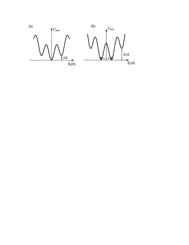
Figure 18: The potential $U_{\rm min}[\theta_{s}(0)]$ at various gate voltages. (a) At $\cos(\pi{\cal N})>0$ the potential has one minimum (spin singlet state). (b) At $\cos(\pi{\cal N})<0$ the minimum is double-degenerate (spin doublet state). Tunneling between the two minima corresponds to the hybridization of the spin states of the dot and lead. This hybridization and consequent lifting of the degeneracy essentially is the Kondo effect.

The “kinetic” part $K\{\phi_{s}\}$ of the Hamiltonian $\hat{H}^{s}$ is quadratic in $\nabla\phi_{s}$, see Eq. (217); it does not commute with the “potential” part, and causes tunneling between the potential minima. The tunneling amplitude is energy-dependent [141], and small at $E\ll T_{0}({\cal N})$. To describe the low-energy dynamics of the spin mode, it is convenient to project out all the states of the Luttinger liquid that are not pinned to the minima of the potential (225). Transitions within one of the sets (4.2) then can be described [140] by a tunneling Hamiltonian

$$\hat{H}_{\pm}=-\frac{\tilde{D}^{2}}{2\pi T_{0}({\cal N})}\cos\left\{\sqrt{\pi}[\phi_{s}(+0)-\phi_{s}(-0)]\right\},$$ (228)

which operates in an energy band $\tilde{D}\ll T_{0}({\cal N})$. Here a discontinuity of the variable $\phi_{s}(x)$ at $x=0$ is allowed, and the point $x=0$ is excluded from the region of integration in Eq. (217). The Hamiltonian $\hat{H}_{xy}$, which is a sum of two operators of finite shifts for the field $\theta_{s}(0)$, represents hops $\theta_{s}(0)\to\theta_{s}(0)\pm\sqrt{\pi}$ between pinned states. In other words, $\hat{H}_{\pm}$ is the finite shift operator with respect to the variable $\theta$ as can be checked with the help of the commutation relations (210).

These hops correspond to a change by $1$ of the $z$–projection of the dot’s spin. At energy scales ${\tilde{D}}\gg\Delta$ the hops are predominantly inelastic. The variation of the transition amplitude with energy can be found by continuing the same RG procedure, until the running cut-off ${\tilde{D}}$ reaches the value $\Delta$. At energies below $\Delta$, fluctuations which involve the excitations of spin mode in the dot ($0<x<L$) are suppressed. If the minimum of energy (225) is non-degenerate (spin-singlet state of the dot), then only one spin state in the dot remains available. However, in the case $\cos(\pi{\cal N})<0$, there is an exact degeneracy between two lowest-energy states, see Fig. 18; the ground state is a spin-doublet. The Hamiltonian (228) hybridizes the spin of the dot with the continuum of spin excitations in the lead. The Kondo effect consists essentially of this hybridization, which lifts the degeneracy and ultimately leads to the formation of a spin singlet in the entire system. The energy scale at which the hybridization occurs, is the Kondo temperature of the problem at hand.

Note that Eq. (228) does not contain any unknown numerical factor. Finding the multiplicative factor in (228) cannot be done within the RG treatment we presented above. To find the numerical constant, one has to use [135] the exact result [140, 40] for the linear response of an unconstrained ($L\to\infty$) Luttinger liquid with $g=1/2$. Matching the low-temperature asymptote of the exact result with the result of the calculation based on the tunneling Hamiltonian formalism, we were able to find the constant in Eq. (228). Also, we would like to notice that the initial Hamiltonian (208), (209), (211) commutes with the total spin of the system: scattering in the junction, represented by the Hamiltonian (209), is clearly spin-conserving. The spin Hamiltonian (217)–(218), obtained after the charge mode was integrated out, also preserves the total spin. However, the tunneling Hamiltonian (228) has the symmetry of the operator $S_{x}(-0)S_{x}(+0)+S_{y}(-0)S_{y}(+0)$, and represents the in-plane part of exchange between the spin densities of the lead and dot [$S(+0)$ and $S(-0)$, respectively] at the point of contact. To restore the $SU(2)$ symmetry of the Hamiltonian, we must supplement $\hat{H}_{\pm}$ with another term, which represents the Ising component of the exchange interaction:

$$\hat{H}_{z}=\frac{v_{F}^{2}}{2T_{0}({\cal N})}\nabla\theta_{s}(-0)\nabla\theta_{s}(+0).$$ (229)

This term is omitted usually in the DC tunneling problem for a Luttinger liquid [140]. In agreement with the general idea about $SU(2)$ symmetry of the $g=1/2$ Luttinger liquid [142], both operators (228) and (229) have the same scaling dimension. To find the numerical factor in Eq. (229), again a comparison with the exact solution is necessary.

We have seen in this Subsection, that there is a hierarchy of the energy scales characterizing an open dot. The charge of the dot fluctuates only at energy scales exceeding $E_{c}$; at lower energies these fluctuations are suppressed. However, strong fluctuations of the spin of the dot continues down to lower energies, $T_{0}({\cal N})$ see Eq. (223). If $T_{0}({\cal N})$ exceeds the level spacing $\Delta$, then at energies $\Delta\>{{}^{{}_{\displaystyle<}}_{\displaystyle\sim}}\>\varepsilon\>{{}^{{}_{\displaystyle<}}_{\displaystyle\sim}}\>T_{0}({\cal N})$ the spin of the dot is quantized, and may change only in quanta of $\delta S=1$ due to the exchange interaction with the electrons in the lead; at the same time, presence of many intra-dot excitations (electron-hole pairs) is allowed. Finally, at energies below $\Delta$ the intra-dot excitations are also suppressed. Under these conditions, the spin of the dot is $S=0$ or $S=1/2$, depending on the sign of $\cos\pi{\cal N}$. If this cosine is positive, then the dot is in a singlet state, and there are no peculiarities in the temperature dependence of observable quantities at $T\>{{}^{{}_{\displaystyle<}}_{\displaystyle\sim}}\>\Delta$. However, if $\cos\pi{\cal N}<0$, then the dot carries a spin, and the Kondo effect develops at sufficiently low temperatures. In the next Subsection we will study the temperature domain $T\>{{}^{{}_{\displaystyle<}}_{\displaystyle\sim}}\>\Delta$, find the Kondo temperature, and discuss the transport properties of the dot in Kondo regime. Starting from Subsection 4.4, we return to the intermediate temperature scale, $\Delta\>{{}^{{}_{\displaystyle<}}_{\displaystyle\sim}}\>T\>{{}^{{}_{\displaystyle<}}_{\displaystyle\sim}}\>E_{c}$, in order to discuss the dominant transport mechanisms there.

4.3 The limit of low temperature: The effective exchange Hamiltonian and Kondo effect

We could continue using the same RG method applied to the bosonized representation of the Hamiltonian, down to scale ${\tilde{D}}\sim\Delta$; it would allow us to estimate the order of magnitude of the effective exchange constant $J$ responsible for the hybridization. It is possible, however, to develop a different method applicable in the energy domain $T_{0}({\cal N})\>{{}^{{}_{\displaystyle>}}_{\displaystyle\sim}}\>{\tilde{D}}\>{{}^{{}_{\displaystyle>}}_{\displaystyle\sim}}\>\Delta$, which allows us a more accurate determination of $J$ and of the Kondo temperature $T_{K}$.

At energies $E\ll T_{0}({\cal N})$, the spin field $\theta_{s}(0)$ is pinned at the point contact. Recalling that $\theta_{s}(L)=0$, we see that the spin of the dot indeed takes discrete values only, as was mentioned above. At such energy scale, it is instructive to return to the fermionic description of the problem. After the two parts of the Hamiltonian, Eqs. (228) and (229), are found, one can explicitly see that the initial $SU(2)$ symmetry of the problem is preserved. Therefore, the effective Hamiltonian controlling the spin degrees of freedom of the system dot$+$lead at low energies, corresponds to the isotropic exchange interaction,

$$\hat{H}_{\rm ex}=J(\tilde{D}){\hat{\vec{S}}}{\hat{\vec{S}}}_{d}.$$ (230)

Here ${\hat{\vec{S}}}_{d}={\textstyle\frac{1}{2}}\hat{\chi}^{\dagger}_{\sigma_{1}}({\vec{R}}_{0}){\vec{\sigma}}_{\sigma_{1}\sigma_{2}}\hat{\chi}_{\sigma_{2}}({\vec{R}}_{0})$ and ${\hat{\vec{S}}}={\textstyle\frac{1}{2}}\hat{\psi}^{\dagger}_{\sigma_{1}}({\vec{R}}_{0}){\vec{\sigma}}_{\sigma_{1}\sigma_{2}}\hat{\psi}_{\sigma_{2}}({\vec{R}}_{0})$ are the operators of spin density in the dot and in the lead respectively, at the point ${\vec{R}}_{0}$ of their contact; ${\vec{\sigma}}_{\sigma_{1}\sigma_{2}}$ are the Pauli matrices. In what follows, we adopt this point to be the origin, ${\vec{R}}_{0}=0$. The dimension of the exhange constant $J(\tilde{D})$ depends on the way we normalize the electron wave functions; dimension-wise, it can be written as $J(\tilde{D})\propto\left[\nu_{d}\nu T_{0}\right]^{-1}$, where $\nu_{d}$ and $\nu$ are the densities of states in the dot and lead, respectively.

In fact, the form of the Hamiltonian (230) could be derived without resorting to the explicit calculation performed above within the bosonization technique. The only important notion needed for the derivation, is the low-energy decoupling of the dot from the lead. Pinning of both charge and spin modes is the manifestation of this decoupling. The decoupling is complete, however, only in the absence of excitations. To describe the behavior of the system at low but finite temperatures, one needs to establish the least irrelevant operators that violate the complete decoupling. The decoupled dot and lead are described by independent Fermi liquids. The number of electrons in the dot can not be changed, as such a variation of charge would result in a large energy increase of order $E_{c}$. That is why the leading irrelevant operators preserving the initial $SU(2)$ symmetry are the interaction in the charge and spin channels between the dot and the lead at the point of contact,

$$\hat{H}_{\rm irr}=A(\tilde{D})\hat{\rho}\hat{\rho_{d}}+\hat{H}_{\rm ex},$$

where $\hat{H}_{\rm ex}$ is defined in Eq. (230) and ${\hat{\rho}}_{d}=\hat{\chi}^{\dagger}_{\sigma}({\vec{R}}_{0})\hat{\chi}_{\sigma}({\vec{R}}_{0})$ and ${\hat{\rho}}=\hat{\psi}^{\dagger}_{\sigma}({\vec{R}}_{0})\hat{\psi}_{\sigma}({\vec{R}}_{0})$ are the operators of the charge density in the dot ($x>0$) and in the lead ($x<0$) respectively, at the point ${\vec{R}}_{0}$ of their contact. The first term here represents the interaction in the singlet channel (inelastic scattering between an electron in the dot an electron in the lead). Because the charge fluctuations are suppressed at energy $E_{c}$ which exceeds significantly the pinning energy of the spin mode $r^{2}E_{c}$, one finds $A/J\simeq r^{2}\ll 1$. Therefore, we can neglect the interaction in the singlet channel. Moreover, even if this mode is taken into account, it does not lead to any non-trivial effect at low energies.

The Hamiltonians (228), (229) and (230) describe, in the bosonic and fermionic representation respectively, the low-energy properties of the very same system. Correlation functions of observable quantities, calculated with the help of Eqs. (228), (229) should coincide with the results for the same functions obtained from the calculation which uses Hamiltonian (230), at temperatures $\Delta\ll T\ll T_{0}(\cal{N})$. This fact will enable us to find the exact value of the coupling constant in the Hamiltonian (230). The advantage of the fermionic representation is that it allows for the description of the system at $T\simeq\Delta$ (ultimately leading to the Kondo effect). We turn to this problem now.

We first rewrite the Hamiltonian (230) in the basis of electron eigenfunctions $\varphi_{n}({\bf R})$ and $\varphi_{k}({\bf R})$ in the dot and lead respectively. In this basis, the Hamiltonian takes the form

$$\hat{H}_{\rm ex}=\frac{1}{4}\sum_{\{nk\sigma\}}{\tilde{J}}_{n_{1}n_{2}k_{1}k_{2}}\left(\vec{\sigma}_{\sigma_{1}\sigma_{2}}\vec{\sigma}_{\sigma_{3}\sigma_{4}}\right)c_{n_{1}\sigma_{1}}^{\dagger}c_{n_{2}\sigma_{2}}c_{k_{1}\sigma_{3}}^{\dagger}c_{k_{2}\sigma_{4}}$$ (231)

with the matrix elements ${\tilde{J}}_{n_{1}n_{2}k_{1}k_{2}}=J(\tilde{D})\varphi^{*}_{n_{1}}(0)\varphi_{n_{2}}(0)\varphi^{*}_{k_{1}}(0)\varphi_{k_{2}}(0)$. The detailed structure of the one-electron functions in the continuum of states $\{k\}$ is not important in the discussion of the Kondo effect. An examination of the standard calculation [114] shows that only the densities $|\varphi_{k}(0)|^{2}$, averaged over the continuum of states $k$, matter. Therefore we will suppress the indices $k_{1}$ and $k_{2}$ in the exchange constants hereinafter, assuming that the functions $\varphi_{k}$ are normalized so that

$$|\varphi_{k}(0)|^{2}=\langle|\varphi_{k}(0)|^{2}\rangle=1.$$ (232)

If the dot is in the spin-doublet state, the exchange constant gets renormalized at low energies. Unlike the “ordinary” Kondo model with only one localized orbital state involved, here the renormalization occurs due to virtual transitions in both the continuum spectrum of the lead and the discrete spectrum of the dot. To see the signature of the Kondo effect, we calculate the second order correction to the exchange constant $J_{00}$ where $0$ labels the singly occupied level of the quantum dot.

This second order correction, diagrammatically shown in Fig. 19, has the form

$$\delta J_{00}(E,{\tilde{D}})=J^{2}(\tilde{D})|\varphi_{0}(0)|^{2}\int_{|E|}^{\tilde{D}}\nu d\xi\sum_{|\xi_{d}^{(l)}|<\tilde{D}}\frac{|\varphi_{l}(0)|^{2}}{|\xi|+|\xi_{d}^{(l)}-\xi_{d}^{(0)}|},$$ (233)

where the integral is taken over the continuum energy spectrum $\xi$ in the leads, $\nu$ is the corresponding density of electron states. The sum over the discrete energy levels of electrons in the dot includes the term involving the singly occupied level $l=0$. This term, which corresponds to a spin-flip within the same orbital level, $\xi_{d}^{(0)}=0$, is responsible for the logarithmic singularity in the “ordinary” Kondo effect. The rest of the terms in the sum correspond to the virtual transitions onto (from) the partially occupied level from (to) doubly-occupied (empty) electron levels.

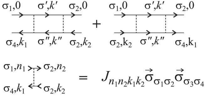
Figure 19: The diagrammatic representation for the second order correction to the exchange interaction constant. The electron states in the intermediate lines include excitations within energy strip $\left[E,\tilde{D}\right]$.

At energies $E\gg\Delta$ the discreteness of the spectrum is not important. If one neglects this discreteness all together the correction to the exchange constant is ultraviolet divergent $\propto\tilde{D}$.

$$\delta J=J^{2}\int_{|E|}^{\tilde{D}}\nu d\xi\int_{-\tilde{D}}^{\tilde{D}}\frac{\nu_{d}d\xi_{d}}{|\xi|+|\xi_{d}|},\quad E\gg\Delta.$$ (234)

Here $\nu_{d}=1/\Delta$ is the one particle density of states in the dot.

This divergent correction is similar to the irreducible vertex function in Fermi liquid theory and can be incorporated into a new constant $J$ which can be numerically different from the bare constant. It is this “new” constant $J$ through which all observables at low energies are expressed. This condition allows us to exclude a large portion of the quasi-continuous spectrum of states in the dot at energies $E\>{{}^{{}_{\displaystyle<}}_{\displaystyle\sim}}\>\tilde{D}$, and to relate the “new” constant $J(E,{\tilde{D}})$ in the fermion Hamiltonian, which is valid at energies $E\ll\tilde{D}$, to the constant in the boson Hamiltonian (228), (229), which does not have free parameters. To establish such a relation, one needs to consider a quantity that does not exhibit strong mesoscopic fluctuations, and therefore can be expressed in terms, insensitive to the particular values of the wave functions $\varphi_{n}(0)$.

The observable quantity to look at, is the spin magnetization of the dot caused by a magnetic field $h_{z}$ applied only to the lead. Application of such a field results in a spin polarization, due to the Pauli susceptibility, of electrons in the lead. This polarization, via the contact interaction, induces a finite spin polarization of the dot. Such a calculation can be performed both in the bosonic and fermionic variables. In the boson variables, the Hamiltonian causing the perturbation of electrons in the lead has the form $\int_{-\infty}^{0}dx\,h_{z}\nabla\theta_{s}(x)$. This form, together with the Hamiltonian of the free spin mode, Eq. (217), allows us to find the induced non-zero value of $\langle\nabla\theta_{s}(0)\rangle\sim h_{z}/v_{F}$. This polarization, in turn, creates a perturbation $[v_{F}h_{z}/T_{0}({\cal N})]\nabla\theta_{s}(+0)$ for the spin mode in the dot, as seen from the Hamiltonian (229). Finally, the spin polarization of the dot $S\equiv\int_{0}^{L}dx\nabla\theta_{s}\sim h_{z}/T_{0}({\cal N})$ can be evaluated by considering the just mentioned perturbation together with the unperturbed Hamiltonian (217). The final result is $L$-independent and thus preserves its meaning in the limit $\Delta\to 0$. In a Fermion representation, one finds $S\sim h_{z}J\nu_{d}\nu$ for the spin of the dot by a straightforward first-order perturbation theory in the exchange Hamiltonian (231). Comparing the two results for $S$, we find

$$J(E,{\tilde{D}})=J\equiv\left[\nu_{d}\nu T_{0}({\cal N})\right]^{-1},\quad\tilde{D}\gg E\gg\Delta.$$ (235)

With the help of Eq. (235) we can relate the constant $J(\tilde{D})$ in the Hamiltonian (230) with $T_{0}({\cal N})$.

After we incorporated all ultraviolet contributions into the definition of the exchange constant, we are ready to study the Kondo effect per se. Taking the difference of Eqs. (233) and (234) to find the second order correction to the “new” coupling constant (235), we find that the correction now only involves a contribution from the difference of the true (discrete) spectrum of the dot and the approximation where the density of states is constant (and continuous):

$$J_{00}=J|\varphi_{0}(0)|^{2} \left[1+J\int_{|E|}^{\tilde{D}}\nu d\xi\left(\sum_{|\xi_{d}^{(l)}|<\tilde{D}}\frac{|\varphi_{l}(0)|^{2}}{|\xi|+|\xi_{d}^{(l)}-\xi_{d}^{(0)}|}\right.\right.$$

$$\left.\left.-\int_{-\tilde{D}}^{\tilde{D}}\frac{\nu_{d}d\xi_{d}}{|\xi|+|\xi_{d}|}\right)\right],$$

where $\nu_{d}=1/\Delta$ is the one particle density of states in the dot. The right hand side of Eq. (4.3) is now perfectly convergent in the high energy. On the other hand, the contribution of the term with $l=0$ gives a logarithmic divergence at $E\to 0$. This is precisely the term which describes the Kondo effect, since it corresponds to a spin flip of an electron on an upper level without excitations of electron-hole pairs in the dot.

We obtain from Eq. (4.3)

$$J_{00}(E,{\tilde{D}})=J|\varphi_{0}(0)|^{2}+J^{2}\nu\left(|\varphi_{0}(0)|^{4}\ln\frac{\Delta}{E}+\Lambda\right),$$ (237)

$$\Lambda=\lim_{\tilde{D}\to\infty}\lim_{E\to 0}\displaystyle\int_{|E|}^{\tilde{D}}\nu d\xi\left[\sum_{|\xi_{d}^{(l)}|<\tilde{D},l\neq 0}\frac{|\varphi_{l}(0)|^{2}}{|\xi|+|\xi_{d}^{(l)}|}-\int_{-\tilde{D}}^{\tilde{D}}\frac{\nu_{d}d\xi_{d}}{|\xi|+|\xi_{d}|}\right].$$ (238)

The limit $E=0$ exists in Eq. (238), and the constant $\Lambda$ is of the order of unity and fluctuates from sample to sample. We will not consider these fluctuations, because fluctuations of the wave function $\varphi_{0}(0)$ controlling the logarithmic Kondo correction to $J_{00}(E,{\tilde{D}})$ lead to much stronger effects. Equation (237) demonstrates that in the strong tunneling regime the bandwidth for the effective Kondo problem at hand is $\Delta$ rather than $E_{c}$. Once Eq. (237) is established, one can obtain, following the lines of [122], the result for Kondo temperature

$$T_{K}\simeq\Delta\sqrt{\frac{\Delta}{T_{0}({\cal N})}}\exp\left\{-\frac{T_{0}({\cal N})}{\alpha\Delta}\right\}$$ (239)

with $T_{0}({\cal N})$ defined in (223) and $\alpha=|\varphi_{0}(0)|^{2}/\langle|\varphi_{0}(0)|^{2}\rangle$. The parameter $\alpha$ is a random quantity obeying Porter-Thomas statistics [59], see Eq. (158).

The above consideration of the Kondo effect in a partially open dot shows us that the low-temperature behavior of the blockaded dot has no qualitative changes with respect to the case of a dot weakly coupled to the leads, as long as

$$E_{c}|r|^{2}\gg\Delta.$$

The only difference developing at larger conductances, is that the parameters defining the low-temperature behavior differ from the bare conductances of the junction. Comparison of the results for Kondo temperature (174) and (239) illustrates this point. In both cases, $T_{K}$ is controlled by the value of $J\nu$,

$$T_{K}\simeq\Delta(J\nu)^{1/2}e^{-1/J\nu}.$$

In the case of strong Coulomb blockade, this parameter is simply related to the conductance of the junctions and to the ratio $E_{c}/\Delta$ by second-order perturbation theory in tunneling amplitudes, see Eq. (174). In the case of strong charge fluctuations, we needed a more sophisticated procedure of renormalization in order to relate $J\nu$ to the bare parameters of the quantum dot, see Eq. (235). The two expressions for the Kondo temperature $T_{K}$ match each other at reflection coefficient $|r|^{2}\simeq 1/2$.

The Kondo effect in a single-junction system results in a specific behavior of the spin polarization. If the dot is in a singlet state, the gap for its spin polarization is $\sim\Delta$. In the doublet state, the contribution of the dot to the susceptibility at low temperature and fields, $T,\mu_{B}H\ll\Delta$, is identical to that of a Kondo impurity [118] with $T_{K}$ given by Eq. (239); here $\mu_{B}$ is the Bohr magneton for the electrons of the dot. The manifestation of the most interesting effect, the enhanced low-temperature conductance, requires a two-junction dot geometry, and we turn to the corresponding discussion now.

Our first goal is to write a fermionic Hamiltonian describing the system at energies so small that, due to the pinning of all charge and spin modes, the Fermi-liquid behavior is already restored. Similar to our discussion after Eq. (230), we obtain such a Hamiltonian using solely the symmetry arguments, and relegate the explicit model calculation to Appendix E.

Once again, the interaction of the charge degrees of freedom of the dot and the lead are suppressed, so we can restrict ourselves to the spin-spin interaction only. The difference from the one-contact geometry, is that now processes which involve two contacts, as well as the ones involving a single contact, are possible. The most general form of the Hamiltonian describing all such processes is

$$\hat{H}_{\rm ex}=\frac{1}{4}\sum_{i,j}J_{ij}{\vec{\sigma}}_{\sigma_{1}\sigma_{2}}{\vec{\sigma}}_{\sigma_{3}\sigma_{4}}\hat{\psi}^{\dagger}_{\sigma_{1},i}({\vec{R}}_{i})\hat{\chi}^{\dagger}_{\sigma_{3}}({\vec{R}}_{j})\hat{\chi}_{\sigma_{4}}({\vec{R}}_{i})\hat{\psi}_{\sigma_{2},j}({\vec{R}}_{j}),$$ (240)

where indices $i,j=1,2$ label the contacts, $J_{ij}=J_{ji}$ are coupling constants, and ${\vec{R}}_{i}$ describes the location of the point contact.

The exchange interaction constants $J_{ij}$ should be found from the calculation of a set of low-energy correlation functions. We can do the explicit evaluation of the constants for the strongly-assymetric set-up, $|r_{1}|\to 1$, $|r_{2}|\ll 1$. In this case, the largest exchange constant $J_{22}$ is determined by the single-junction result, $J_{22}=J$, where $J$ is defined by Eq. (235) with $r_{2}=r$. The constant $J_{12}$, which characterizes the non-local exchange accompanied by the charge transfer, is proportional to $\sqrt{g_{1}}$, and the exchange constant at the weaker junction is $J_{11}\propto g_{1}$, where $g_{1}\sim 1-|r_{1}|^{2}$ is the dimensionless conductance of the weaker junction. As a matter of fact, in the limit of strong asymmetry the numerical coefficients can be found also, with the help of the exact solution [40] available for the case $\Delta=0$. To find $J_{12}$, we can calculate the linear conductance $G(T)$ through the dot using the Hamiltonian (240), and then compare it with the exact result [40]. In the lowest order of the perturbation theory, transitions across the dot are induced by only the terms $\propto J_{12}$ in the Hamiltonian (240). The conductance can be calculated by applying the standard Fermi golden rule to the problem. Because we neglect the level spacing at the moment, and because of the four-fermion structure of the Hamiltonian (240), the electron transition rate and the conductance $G$ at low temperatures is proportional to $T^{2}$,

$$G(T)=\frac{\pi^{3}e^{2}}{4\hbar}J_{12}^{2}\nu^{2}\nu_{d}^{2}T^{2}.$$

The comparison with the exact result [40], see also Eq. (361), yields:

$$J_{12}^{2}=\frac{32}{3\pi^{2}e^{\bf C}}\frac{\pi\hbar}{e^{2}}G_{1}\left[E_{c}T_{0}({\cal N})\nu^{2}\nu_{d}^{2}\right]^{-1}.$$ (241)

The smallest exchange constant in the problem, $J_{11}$, does not affect the conductance in the strongly-assymetric set-up which we consider here. For calculating the conductance in the absence of strong asymmetry, one should know the value of $J_{11}$. For that purpose, some other response function should be calculated with the help of Hamiltonian (240) and then compared with an exact result; we will not address this problem in this Review. Instead, we utilize Eq. (241) to determine the conductance through the dot in the limit of low temperatures. If the gate voltage is close to an odd integer, $\cos\pi{\cal N}<0$, the lowest discrete energy level in the dot is spin-degenerate. At $T\>{{}^{{}_{\displaystyle<}}_{\displaystyle\sim}}\>\Delta$, only this level remains important. This way, the initial problem of the dot, which has a dense spectrum of discrete levels, and is strongly coupled to the leads, is reduced to the problem of a single-level Kondo impurity considered in Section 3.3. We can adapt the result (170) to find the conductance. First, we express the temperature-independent factor in terms of the exchange constants, rather than in terms of the conductances $g_{1}$ and $g_{2}$:

$$\frac{4g_{1}g_{2}}{(g_{1}+g_{2})^{2}}\to\frac{4J_{12}^{2}}{(J_{11}+J_{22})^{2}}.$$

Next, we neglect the small term $J_{11}$ in the denominator here, and find:

$$G_{K}\left(\frac{T}{T_{K}},{\cal N}\right)=\frac{4e^{2}}{\pi\hbar}\left(\frac{J_{12}}{J_{22}}\right)^{2}f\left(\frac{T}{T_{K}}\right).$$

Now we are ready to find the Kondo conductance through the dot in the regime of strong charge fluctuations which we consider in this Section. For that, we substitute the exchange constants (235) and (241) into the above formula,

$$G_{K}\simeq\left(\frac{16}{3}\right)\left(\frac{4}{\pi}\right)^{3}\frac{1024}{3\pi^{3}}G_{1}|r_{2}|^{2}(\cos\pi{\cal N})^{2}f\left(\frac{T}{T_{K}({\cal N})}\right).$$ (242)

Here, $T_{K}({\cal N})$ is given by Eq. (239), and $f(x)$ is the universal scaling function plotted in Fig. 14. Note that the Kondo conductance (242) in a strongly asymmetric set-up is proportional to the product of the small conductance $G_{1}$ and small reflection coefficient $|r_{2}|^{2}$ and therefore is significantly smaller than the conductance quantum $e^{2}/\pi\hbar$ even at $T=0$.

Similar to the case of the closed quantum dot, the dominant mechanisms switch from inelastic co-tunneling at high temperatures to the elastic temperature-independent mechanism at lower temperatures, and finally to the regime of the Kondo effect at the lowest temperatures. We postpone a more detailed discussion of those crossovers until after we have constructed a theory of elastic co-tunneling in open quantum dots. We turn to the outline of this theory in the following subsections.

4.4 Simplified model for mesoscopic fluctuations

As was already mentioned in the beginning of this section, the main difficulty for building a theory of interacting electrons in an open dot stems from the need to treat both the Coulomb interaction and the dot-lead conductance non-perturbatively. In the limit $\Delta\to 0$, the bosonization procedure allows one to treat exactly the interaction in a dot connected to a lead by a perfect quantum channel. Then, the effect of a finite reflection amplitude $r$ in the channel can be treated by a systematic perturbation theory [39, 40]. An important conceptual conclusion drawn from this theory is that in the low-energy sector (defined by $\varepsilon\>{{}^{{}_{\displaystyle<}}_{\displaystyle\sim}}\>E_{c}|r|^{2}$), the excitations inside and outside the dot are independent from each other. This understanding allowed us to consider the low-temperature effects ($T\>{{}^{{}_{\displaystyle<}}_{\displaystyle\sim}}\>\Delta$) in a partially open dot with $E_{c}|r|^{2}\gg\Delta$, because in this case one is able to map the properties of a partially-open dot onto the “conventional” case of strong Coulomb blockade (see the previous subsection). Such a mapping allows one to consider the Kondo effect, but is insufficient for evaluating the co-tunneling contribution to the conductance, for which a broad range of energies up to $E_{c}$ is involved. (This was shown, e.g., in Sec. 3.2, where we considered the valley conductance through a strongly blockaded quantum dot.) The aim of this and the following Sections is to build a theory capable of describing simultaneously many-body effects and mesoscopic fluctuations at the intermediate range of energies, $E_{c}\>{{}^{{}_{\displaystyle>}}_{\displaystyle\sim}}\>\varepsilon\>{{}^{{}_{\displaystyle>}}_{\displaystyle\sim}}\>{\mathrm{m}ax}(E_{c}|r|^{2},\Delta)$. This section deals with a qualitative picture of the role of the mesoscopic fluctuations; a rigorous calculation to verify the qualitative picture below is given in the following sections.

Let us first consider a completely opened channel ($r=0$). In the limit $\Delta\to 0$, the electron charge of the dot varies with the gate voltage as $\langle Q\rangle=e{\cal N}$, to ensure the minimum of the electrostatic energy [39]. The interaction term in Eq. (92) depends only on the number of electrons crossing the dot-channel boundary. Since this information is represented as well in the asymptotic behavior of the wave-functions far from the entrance to the dot, such as the scattering phase shift, the properties of the ground state can be characterized by an analysis of those asymptotes. For the sake of simplicity, we consider the case of a dot connected to a lead by one channel, and consider spinless fermions instead of real electrons with spin. The ground state properties at low energy can then be understood from the following argument.

The entrance of an additional electron with energy $\varepsilon$ (all the energies will be measured from the Fermi level) into the dot requires the charging energy $E_{c}$. Therefore, the electron may spend a time of the order of $\hbar/E_{c}$ in the dot, after which the extra charge accumulated on the dot has to relax. One can distinguish two processes that lead to charge relaxation: (i) elastic process where the same electron leaves the dot, and (ii) inelastic process where another electron is emitted from the dot. At low energies the probability of the inelastic process is small as $(\varepsilon/E_{c})^{2}$, by virtue of the smallness of the phase volume. (The last statement assumes Fermi liquid behavior at low energies and, as we will see later, is valid only for the spinless one-channel case.) Therefore, for $\varepsilon\ll E_{c}$, we may conclude that an incoming electron spends a time of the order $1/E_{c}$ inside the dot, after which it bounces back into the channel without creating excitations. The same consideration is applicable to an electron attempting to leave the dot. The fact that within the energy range $|\varepsilon|\>{{}^{{}_{\displaystyle<}}_{\displaystyle\sim}}\>E_{c}$ from the Fermi level the electron processes are predominantly elastic implies that the low energy properties of the system can be mapped onto a dot effectively decoupled from the channel, that there is a well-defined scattering amplitude from the entrance of the dot, and that the phase of this scattering amplitude is given by the Friedel sum rule

$$\delta=\pi\langle Q\rangle/e=\pi{\cal N}.$$ (243)

Equation (243) can be applied to electrons incident from inside the dot, as well as to electrons incident from the channel. The description outlined here resembles closely Nozieres’ Fermi liquid description of the unitary limit in the one-channel Kondo problem [118].

We now demonstrate that the above considerations are sufficient to reproduce the result

$$E_{g}({\cal N})\simeq|r|E_{c}\cos 2\pi{\cal N},$$ (244)

obtained by Matveev [39] for the ground state energy $E_{g}({\cal N})$ of spinless fermions in the limit of zero level spacing $\Delta$ in the dot and with a finite reflection amplitude $r$ in the contact, and then apply the same scheme to find the corrections to the ground state energy arising from a finite $\Delta$, but without $r$. Those corrections will result in the mesoscopic fluctuations of the ground state energy.

We start with the limit $\Delta=0$. First, we put $r=0$ and calculate the density of electrons in the channel $\rho(x)$. As we discussed, the Coulomb interaction leads to a perfect reflection of electron at low energies; the wavefunctions have the form $\psi_{k}(x)=\cos\left(k|x|-\delta\right)$, with phase shift $\delta$ given by Eq. (243). This form of the wavefunctions leads to the Friedel oscillation of the electron density

$$\rho(x)=\sum_{v_{F}|k-k_{F}|\>{{}^{{}_{\displaystyle<}}_{\displaystyle\sim}}\>E_{c}}\left|\psi_{k}(x)\right|^{2},$$

where $v_{F}$ and $k_{F}$ are the Fermi velocity and Fermi wavevector respectively. (Here we omitted the irrelevant constant part of the electron density; the restriction of wave vectors $k$ to the range $E_{c}/v_{F}$ around $k_{F}$ is because only for those wavevectors elastic reflection from the contacts takes place.) We thus obtain

$$\rho(x)=\left\{\begin{array}[]{ll}\displaystyle{\frac{E_{c}}{v_{F}}\cos(2k_{F}|x|-2\delta)},&|x|<v_{F}/E_{c},\\ \displaystyle{\frac{\sin(2k_{F}|x|-2\delta)^{\vphantom{M^{M}}}}{|x|}},&|x|>v_{F}/E_{c}.\\ \end{array}\right.$$ (245)

Next, we take into account the effect of a scattering potential $V(x)$ in the contact that generates a finite reflection amplitude $r\neq 0$. In the first order of perturbation theory, the presence of the potential $V$ gives a shift to the ground state energy given by

$$E_{g}({\cal N})=\int dx\rho(x)V(x).$$ (246)

Substituting Eq. (245) into Eq. (246), assuming that the effective range of the potential around $x=0$ is smaller than $v_{F}/E_{c}$, and using the standard expression $|r|=|\tilde{V}(2k_{F})|/v_{F}$, we obtain Eq. (244). Here $\tilde{V}(k)$ is the Fourier transform of the potential $V(x)$.

Having verified the relation between scattering phase shifts and the ground state energy for the case $\Delta=0$, we proceed with evaluation of the ground state energy of a finite dot connected to a reservoir by a perfect channel. According to the discussion preceding Eq. (243), the channel is effectively decoupled from the dot due to the charging effect even though $r=0$. We now find the ground state energy of the system by relating the ground state energy of the closed dot to the scattering phase $\delta$ of Eq. (243). For a chaotic dot, this problem is equivalent to finding a variation of the eigenenergies by introduction of an arbitrary scatterer [143] with the same phase shift $\delta$. The relevant contribution to the ground state energy is given by

$$E_{g}=\sum_{-E_{c}\>{{}^{{}_{\displaystyle<}}_{\displaystyle\sim}}\>\xi_{i}<0}\left[\xi_{i}(\delta)+\mu\right],$$ (247)

where $\xi_{i}$ are the eigenenergies measured from the Fermi level $\mu$. (Again, we have restricted the summation to a window of size $\sim E_{c}$ around the Fermi level, since the phase shift $\delta$ applies only to particles in this energy range.) As soon as the scattering phase changes by $\pi$, one more level enters under the Fermi level. Evolution of the energy levels with changing $\delta$ is shown schematically in Fig. 20. The position of the level $\xi_{i}(\delta)$ satisfies the gluing condition

$$\xi_{i}(\delta+\pi)=\xi_{i+1}(\delta).$$ (248)

From Eqs. (247) and Eq. (248) we see that the ground state energy depends almost periodically on $\delta$:

$$E_{g}(\delta)=E_{g}(\delta+\pi)+{\cal O}(\Delta).$$ (249)

As we will see below, the amplitude of the oscillation of the ground state energy with the variation of $\delta$ is much larger than the mean level spacing, so that we can neglect the last term in Eq. (249).

In order to estimate the magnitude of the oscillations of the ground state energy, we recall that the correlation function of the level velocities is given by [47]

$$\langle\partial_{\delta}\varepsilon_{i}\rangle=\frac{\Delta}{\pi},\quad\langle\partial_{\delta}\varepsilon_{i}\partial_{\delta}\varepsilon_{j}\rangle=\delta_{ij}\frac{2}{\beta}\left(\frac{\Delta}{\pi}\right)^{2},$$ (250)

where $\beta=1,2$ for the orthogonal and unitary ensembles respectively, and $\langle\dots\rangle$ stands for the ensemble averaging. Formula (250) can be easily understood from the first order perturbation theory: At $\delta\ll 1$, we have $\varepsilon_{i}(\delta)\approx\varepsilon_{i}(0)+(\delta/\pi\nu)|\psi_{i}^{2}(0)|$. Using the fact that $\psi_{i}(0)$ is a Gaussian random variable, see Eq. (21), one obtains Eq. (250).

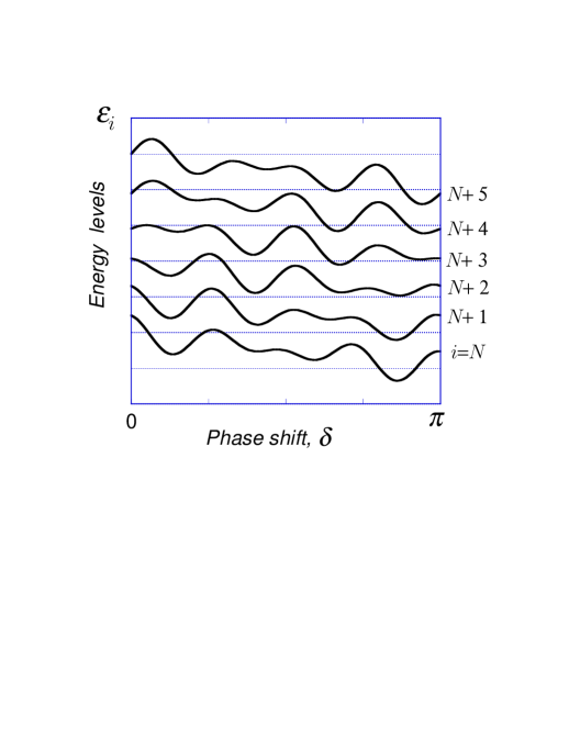
Figure 20: Evolution of the energy levels of the quantum dot with the scattering phase $\delta$.

Estimating the mesoscopic fluctuations of the ground state energy (247) with the help of Eq. (250), we obtain for $\delta\ll 1$

$$\langle\left[E_{g}(\delta)-E_{g}(0)\right]^{2}\rangle=\quad\Delta^{2}\left(\frac{\delta}{\pi}\right)^{2}\sum_{-E_{c}\>{{}^{{}_{\displaystyle<}}_{\displaystyle\sim}}\>\xi_{i},\xi_{j}<0}\frac{2}{\beta}\delta_{ij}\approx{\Delta E_{c}{\delta}^{2}\over\beta}.$$ (251)

As we have already explained, the energy (247) is a periodic function of $\delta$ with period $\pi$. On the other hand, for $\delta\>{{}^{{}_{\displaystyle<}}_{\displaystyle\sim}}\>1$, Eq. (251) is valid. Therefore the characteristic amplitude of the oscillations is of the order of $\sqrt{E_{c}\Delta}$, and it is plausible to assume that the correlation function of energies at two different parameters ${\cal N}_{1},\ {\cal N}_{2}$ takes the form

$$\langle E_{g}\left({\cal N}_{1}\right)E_{g}\left({\cal N}_{2}\right)\rangle\approx{\Delta E_{c}\over\beta}\cos 2\pi\left({\cal N}_{1}-{\cal N}_{2}\right),$$ (252)

where we use Eq. (243). It is important to notice that the variation of the energy of the ground state is much larger than the mean level spacing $\Delta$.

A different, though equivalent way to arrive at Eq. (252) is as follows. We have seen that because of the presence of the charging energy $E_{c}$, charge excitations in the dot relax elastically after a time $\sim\hbar/E_{c}$. If the dot size is infinitely big (corresponding $\Delta=0$), no backscattering from the dot’s walls occurs within this short time interval, and the only source of elastic scattering is an eventual reflection amplitude $r$ in the contact. However, if the dot has a finite size, there is a finite probability that the incoming particle will scatter from its walls, or from impurities inside the dot, and exit elastically before the time $\hbar/E_{c}$. The corresponding amplitude $r$ for reflection from the dot in a time shorter than $\hbar/E_{c}$ can be estimated as

$$r\sim\int_{0}^{\hbar/E_{c}}dtS(t),$$ (253)

where $S(t)$ is the scattering matrix of the dot in time representation, cf. Eq. (121). Hence, in order to include elastic scattering from the dot, we have to add the amplitude (253) to the reflection amplitude $r_{c}$ from the contact in Eq. (244). The mesoscopic fluctuations of $E_{g}$ can then be found from Eq. (124) for the mesoscopic fluctuations of $S(t)$. One verifies that Eq. (252) is quickly recovered.

From the present derivation, it is clear that the charging energy $E_{c}$ enters into the final estimate (252) as an energy scale below which the dot is effectively closed. All higher lying energy levels are not sensitive to the charging energy, and hence not to the gate voltage ${\cal N}$. A similar picture holds also for “real” electrons with spin. As we discussed in Sec. 4.2, see Eq. (223), in that case the dot effectively closes at the much lower energy scale $E_{c}|r|^{2}$. As a result, the amplitude of fluctuations for spin-$1/2$ fermions acquires additional factor $r^{2}$, compared to Eq. (252). Such an estimate is valid unless the reflection coefficient $|r|^{2}$ becomes smaller than $\Delta/E_{c}$. We will see later that in the case of a perfectly transmitting channel ($r=0$), the energy scale $E_{c}|r|^{2}$ should be replaced by $\simeq\Delta\ln\left(E_{c}/\Delta\right)$.

A magnetic field applied to the system affects the states in the dot. Therefore, the ground state energy and, as we will see later, conductance through the dot varies with the field. The corresponding correlation magnetic field flux $\Phi_{c}$ is determined by the number of levels that fit into the energy strip of one-particle levels “blocked” inside the dot. An estimate of $\Phi_{c}$ can be obtained from Eq. (163) with $E$ replaced by $E_{c}$ or $E_{c}|r|^{2}$ for spinless or spin-$1/2$ fermions, respectively.

4.5 Rigorous theory of mesoscopic fluctuations: formalism for multichannel junctions

4.5.1 Derivation of the effective action

We now proceed with an exposition of the general formalism used to calculate the capacitance, tunneling density of states, and conductance of an interacting quantum dot, without neglecting the effect of mesoscopic fluctuations of the wavefunction in the dot. (That is, without neglecting the possibility that an electron that has entered the dot will return coherently to the point contact.) The first step is to reformulate the problem in terms of an effective action that accounts for these coherent returns.

Our formal starting point is the same as in Sec. 2.4: The Hamiltonian of the dot connected to the leads is written as the sum of a Hamiltonian of the closed dot, a Hamiltonian of the leads, and a term $\hat{H}_{LD}$ coupling the lead and the dot,

$$\hat{H}=\hat{H}_{D}+\hat{H}_{\rm C}+\hat{H}_{L}+\hat{H}_{LD}.$$ (254)

Here, the Hamiltonian of the dot is, in turn, written as a sum of the Hamiltonian $\hat{H}_{D}$ of the closed dot in the absence of electron-electron interactions and the charging energy $\hat{H}_{C}$ [see also Eq. (92); here spin is included in the indices $\alpha$ and $\gamma$]

$$\hat{H}_{D}=\sum_{\alpha,\gamma}{\cal H}_{\alpha\gamma}\hat{\psi}^{\dagger}_{\alpha}\hat{\psi}_{\gamma},\quad\hat{H}_{\rm C}=E_{c}\left(\hat{n}-{\cal N}\right)^{2}.$$ (255)

The Hamiltonian $\hat{H}_{L}$ of the leads is given by Eq. (96); the term $\hat{H}_{LD}$ that couples the dot with the leads is given in Eq. (97).

The operator $\hat{n}$ in Eq. (255) is for the total charge $e\hat{n}$ on the dot. Conventionally, it is defined in terms of the creation and annihilation operators $\hat{\psi}^{\dagger}_{\alpha}$ and $\hat{\psi}_{\alpha}$ of fermions in the dot, as in Eq. (34). For the purpose of the formal manipulations of this section, it is more convenient, however, to change the definition (34) of $\hat{n}$, and reformulate it in terms of the operators $\hat{\psi}^{\dagger}_{j}(k)$ and $\hat{\psi}_{j}(k)$ for the channel. This is possible, because the total number of particles in the entire system (leads and dot) is an integer number which can be added to the parameter ${\cal N}$ at no cost, so that we can write

$$\hat{n}=-\sum_{j=1}^{N_{\rm ch}}\int{dk\over 2\pi}\hat{\psi}^{\dagger}_{j}(k)\hat{\psi}_{j}(k).$$ (256)

Strictly speaking, the use of Eq. (256) instead of (34) is only permitted for a canonical description, in which the total number of particles in the system is held fixed. Below, however, we use Eq. (256) in a grand canonical description. The difference between the two descriptions is only important if non-periodic fluctuations as a function of ${\cal N}$ are considered. The modifications of the theory in this case are discussed in Appendix F.

We now discuss the derivation of the effective action separately for the three cases of interest.

Free energy and differential capacitance. To calculate the ground state energy, we start with the thermodynamic potential,

$$\Omega=-T\ln\left({\rm Tr}e^{-\hat{H}/T}\right).$$ (257)

We evaluate the trace in two steps, ${\rm Tr}\dots={\rm Tr}_{L}{\rm Tr}_{D}\dots$, where $L$ and $D$ indicate the fermionic operators belonging to the leads and dot respectively. With the redefinition (256) of the charge $\hat{n}$, the interaction Hamiltonian $H_{C}$ is now attributed to the leads. As a result, the Hamiltonian of the system becomes quadratic in the fermionic operators of the dot, so that this part of the system can be integrated out:

$${\rm Tr}_{D}\,e^{-\hat{H}/T} = {\rm Tr}_{D}\,e^{-\left(\hat{H}_{L}+\hat{H}_{\rm C}+\hat{H}_{D}+\hat{H}_{LD}\right)/T}$$

$$= \ \ e^{-\left(\hat{H}_{L}+\hat{H}_{\rm C}\right)/T}e^{-\Omega_{D}/T}T_{\tau}e^{\frac{1}{2}\int_{0}^{1/T}d\tau_{1}d\tau_{2}\langle\hat{H}_{LD}(\tau_{1})\hat{H}_{LD}(\tau_{2})\rangle_{D}}.$$

Here $\hat{H}_{LD}(\tau)$ is the interaction representation of the dot-lead coupling operator

$$\hat{H}_{LD}(\tau)=e^{\tau(\hat{H}_{L}+\hat{H}_{\rm C}+\hat{H}_{D})}\hat{H}_{LD}e^{-\tau(\hat{H}_{L}+\hat{H}_{\rm C}+\hat{H}_{D})},$$

$T_{\tau}$ denotes time ordering for the imaginary time $\tau$, $\Omega_{D}$ is the thermodynamic potential of the closed dot,

$$\Omega_{D}=-T\ln{\rm Tr}e^{-\hat{H}_{D}/T},$$ (259)

and the average $\langle\ldots\rangle_{D}$ over the Hamiltonian $H_{D}$ of the dot is defined as

$$\langle\dots\rangle_{D}=e^{\Omega_{D}/T}{\rm Tr}_{D}\left(e^{-\hat{H}_{D}/T}\dots\right).$$

Note that, as the interaction has been shifted to the leads, the thermodynamic potential $\Omega_{D}$ of the closed dot is formally independent of the gate voltage ${\cal N}$.

It remains to compute the average $\langle\hat{H}_{LD}(\tau_{1})\hat{H}_{LD}(\tau_{2})\rangle_{D}$ in Eq. (4.5.1). Hereto we use the explicit form (97) of ${\hat{H}}_{LD}$ and the Green function ${\cal G}_{\alpha\beta}(\tau)$ of the closed dot,

$${\cal G}_{\alpha\beta}(\tau)\equiv-\langle T_{\tau}\,\hat{\psi}_{\alpha}(\tau)\hat{\bar{\psi}}_{\beta}(0)\rangle_{D}=T\sum_{n=-\infty}^{\infty}e^{-i\omega_{n}\tau}\left({1\over i\omega_{n}-{\hat{H}}_{D}}\right)_{\alpha\beta},$$ (260)

where $\omega_{n}=\pi T(2n+1)$ is a fermionic Matsubara frequency and $\hat{\bar{\psi}}(\tau)=\hat{\psi}^{\dagger}(-\tau)$. Hence we find

$$\langle\hat{H}_{LD}(\tau_{1})\hat{H}_{LD}(\tau_{2})\rangle_{D} = -2\sum_{j_{1},j_{2}}\hat{\bar{\psi}}_{j_{1}}(\tau_{1},0)\left[W^{\dagger}{\cal G}(\tau_{1}-\tau_{2})W\right]_{j_{1}j_{2}}\hat{\psi}_{j_{2}}(\tau_{2},0),$$

where the operators $\hat{\psi}_{j}(\tau,x)$ are the Fourier transform of $\hat{\psi}_{j}(\tau,k)$,

$$\hat{\psi}_{j}(x)=\int{dk\over 2\pi}e^{-ikx}\hat{\psi}_{j}(k).$$

It is convenient to introduce a new matrix, $L_{j_{1}j_{2}}$, by the following relation:

$$4L(i\omega_{n})_{j_{1}j_{2}}\equiv-{\mbox{sign}\,\omega_{n}\over i\pi\nu}\delta_{{j_{1}j_{2}}}+\left[W^{\dagger}{\cal G}(i\omega_{n})W\right]_{j_{1}j_{2}},$$ (262)

where $\nu=1/2\pi v_{F}$ is the density of states in the leads. With this definition, the dot Green function ${\cal G}$ and the coupling matrix $W$ can be eliminated from Eq. (LABEL:eq:HH) in favor of the matrix $L$, so that we obtain

$$\langle\hat{H}_{LD}(\tau_{1})\hat{H}_{LD}(\tau_{2})\rangle_{D} = {2T\over\pi\nu\sin[\pi T(\tau_{1}-\tau_{2})]}\sum_{j}\hat{\bar{\psi}}_{j}(\tau_{1},0)\hat{\psi}_{j}(\tau_{2},0)$$ (263)

$$\mbox{}-{1\over 2}\sum_{j_{1},j_{2}}\hat{\bar{\psi}}_{j_{1}}(\tau_{1},0)L_{j_{1}j_{2}}(\tau_{1}-\tau_{2})\hat{\psi}_{j_{2}}(\tau_{2},0).$$

The first term in the r.h.s. comes from the diagonal part of the Green function ${\cal G}$ (i.e., the density of states in the dot); this term can be obtained by multiplying the ensemble-averaged Green function by the product $W^{\dagger}W=\pi^{2}\nu/M\Delta$ characterizing an ideal dot-lead coupling. The second term, which contains the matrix $L_{j_{1},j_{2}}$, also has components off-diagonal in $j_{1}$ and $j_{2}$. It accounts for a combined effect of electron trajectories backscattered into the lead. Backscattering may be caused by electron reflection off a barrier in the contact, impurities in the contact and the dot, and the boundaries of the dot. This term is responsible for the mesoscopic fluctuations of the observable quantities.

Except for the average density of states, the first term in Eq. (263) does not contain information about the dot. We could have obtained the very same term if the coupling to the dot would have been replaced by an ideal coupling of each chiral fermion field $\hat{\psi}_{j}(x)$ in the lead to a free chiral fermion field $\hat{b}_{j}(x)$. Writing these fields explicitly, we find that Eq. (4.5.1) takes the form

$$\mbox{Tr}_{D}e^{-\hat{H}/T}\propto\mbox{Tr}_{b}\,e^{-\Omega_{D}/T}e^{-\hat{H}_{\rm eff}/T}T_{\tau}e^{-{\cal S}_{\rm eff}}$$ (264)

where $\mbox{Tr}_{b}$ denotes a trace over the chiral fermion fields $\hat{b}_{j}$, $\hat{H}_{\rm eff}$ is an effective Hamiltonian that contains the fermion fields $\hat{\psi}_{j}(x)$ in the lead, the fictitious fermion fields $\hat{b}_{j}(x)$, and their coupling at $x=0$,

$$\hat{H}_{\rm eff} = iv_{F}\sum_{j}\int{dx}\,\left[\hat{\psi}^{\dagger}_{j}(x)\partial_{x}\hat{\psi}_{j}(x)+\hat{b}^{\dagger}_{j}(x)\partial_{x}\hat{b}_{j}(x)\right]$$ (265)

$$\mbox{}+\frac{1}{\pi\nu}\sum_{j}\left[\hat{b}_{j}^{\dagger}(0)\psi_{j}^{\vphantom{X}}(0)+\psi_{j}^{\dagger}(0)\hat{b}_{j}^{\vphantom{X}}(0)\right]$$

$$\mbox{}+E_{c}\left(\sum_{j}\int dx:\!\hat{\psi}^{\dagger}_{j}(x)\hat{\psi}_{j(x)}\!:+{\cal N}\right)^{2},$$

and ${\cal S}_{\rm eff}$ is an effective action that contains the fields $\hat{\psi}_{j}(x)$ at $x=0$ only,

$${\cal S}_{\rm eff}=4\sum_{j_{1},j_{2}}\int_{0}^{1/T}d\tau_{1}\int_{0}^{1/T}d\tau_{2}\hat{\bar{\psi}}_{j_{1}}(\tau_{1};0)L_{j_{1}j_{2}}(\tau_{1}-\tau_{2})\hat{\psi}_{j_{2}}(\tau_{2};0).$$ (266)

The equivalence of the representations (4.5.1) and (264) – (266) can be easily checked by tracing out the fermions $\hat{b}_{j}$ in Eq. (264), with the help of the relation [cf. the first term on the r.h.s. of Eq. (262)]

$$\langle T_{\tau}\hat{b}_{j_{1}}(\tau;0)\hat{\bar{b}}_{j_{2}}(0;0)\rangle=i\pi\nu T\delta_{j_{1}j_{2}}\sum_{\omega_{n}}e^{-i\omega_{n}\tau}{\rm sgn}\,\omega_{n}.$$

The operators $\hat{\psi}_{j}(0)$ and $\hat{b}_{j}(0)$ appearing in the effective Hamiltonian (265) and in the effective action (266) are the fermion fields evaluated at the origin $x=0$. To simplify notation, from now on we omit the coordinate in the argument of the one-dimensional operators $\psi_{j}$ (or, later, of the bosonic operators $\phi_{j}$), when they are taken at the origin,

$${\psi}_{j}(\tau)\equiv{\psi}_{j}(\tau;x=0),\quad{\phi}_{j}(\tau)\equiv{\phi}_{j}(\tau;x=0).$$ (267)

It can be checked that the operator in the second line of Eq. (265) connecting the fermion fields $\hat{\psi}$ and $\hat{b}$ at $x=0$ corresponds to an ideal coupling between those fields. This coupling means that a $\psi$-particle is scattered to a $b$-particle with unit probability. This motivates the following substitution of right and left moving fermion fields,

$$\hat{\psi}_{j}(x) = \hat{\psi}_{L,j}(x)\theta(-x)+\hat{\psi}_{R,j}(-x)\theta(x),$$

$$\hat{b}_{j}(x) = i\left[\hat{\psi}_{R,j}(-x)\theta(-x)-\hat{\psi}_{L,j}(x)\theta(x)\right].$$ (268)

[Here $\theta(x)=1$ if $x>0$, $0$ if $x<0$, and $\theta(0)=1/2$.] With this substitution we obtain from Eqs. (265) – (266)

$$\hat{H}_{\rm eff} = iv_{F}\sum_{j}\int_{-\infty}^{\infty}dx\left(\hat{\psi}^{\dagger}_{L,j}\partial_{x}\hat{\psi}_{L,j}-\hat{\psi}^{\dagger}_{R,j}\partial_{x}\hat{\psi}_{R,j}\right)$$ (269)

$$\mbox{}+{E_{c}}\left(\sum_{j}\int_{-\infty}^{0}dx:\!\hat{\psi}^{\dagger}_{L,j}\hat{\psi}_{L,j}+\hat{\psi}^{\dagger}_{R,j}\hat{\psi}_{R,j}\!:+{\cal N}\right)^{2},$$

$${\cal S}_{\rm eff} = \sum_{j_{1}j_{2}}\int_{0}^{1/T}d\tau_{1}\int_{0}^{1/T}d\tau_{2}\,L_{j_{2}j_{2}}\left(\tau_{1}-\tau_{2}\right)$$ (270)

$$\mbox{}\times\left[\hat{\bar{\psi}}_{L,j_{1}}(\tau_{1})+\hat{\bar{\psi}}_{R,j_{1}}(\tau_{1})\right]\left[\vphantom{\hat{\bar{\psi}}_{L,j_{1}}}\hat{\psi}_{L,j_{2}}(\tau_{2})+\hat{\psi}_{R,j_{2}}(\tau_{2})\right],$$

where the time dependence of any operator $\hat{A}$ is defined as

$$\hat{A}(\tau)=e^{\tau\hat{H}_{\rm eff}}\hat{A}e^{-\tau\hat{H}_{\rm eff}}.$$ (271)

In this formulation, all backscattering from the dot and from the contact is characterized by the kernel $L$. To make contact with the theory of Sec. 2.4 of a non-interacting quantum dot, it is advantageous to express $L$ in terms of the scattering matrix $S$ of the non-interacting system. Comparing Eqs. (101) with Eq. (262), one immediately finds

$$L(\omega_{n})=\int_{0}^{1/T}e^{i\omega_{n}\tau}L(\tau)d\tau=\left\{\matrix{\displaystyle-{1\over 2\pi i\nu}\frac{S(i\omega_{n})}{1+S(i\omega_{n})_{\vphantom{M}}},&\omega_{n}>0,\cr\displaystyle{1\over 2\pi i\nu}\frac{S^{\dagger}(i\omega_{n})^{\vphantom{M^{M}}}}{1+S^{\dagger}(i\omega_{n})},&\omega_{n}<0.}\right.$$ (272)

This relation allows us to deduce the statistical distribution of the kernel $L(\tau)$ from the better known statistical distribution of the scattering matrix $S$, see Sec. 2.4. For ideal contacts the ensemble average of $S^{n}$ (with integer $n$) is zero, cf. Eq. (117), which implies that the ensemble average of $L$ is zero as well.

Equations (269) and (270) provide an effective description of the combined system of the lead and the dots in terms of fermions moving in one-dimensional wires, where the interaction only exists on one end of the wire. The effective action ${\cal S}_{\rm eff}$ provides a coupling between the wires and between left and right moving fermions. The one dimensional description for the charging effect, which was already introduced in Sec. 4.2, was first proposed by Flensberg [38] and Matveev [39]. Their theory can be interpreted as an approximation of the effective action theory presented here, corresponding to the replacement of $S$ (and $L$) by its ensemble average,

$$S_{j_{1}j_{2}}\to\langle S_{j_{1}j_{2}}\rangle=-ir_{j_{1}}\delta_{j_{1}j_{2}},$$ (273)

where $r_{j}$ is the backscattering amplitude in the contact for the $j$-th channel, see Sec. 2.4. At weak backscatterring, $r_{i}\ll 1$, Eq. (272) gives, cf. Eq. (123),

$$L_{ij}(\tau)=v_{F}\delta(\tau)\delta_{ij}r_{j},$$ (274)

so that the action loses its time dependence and acquires the form of a backscattering Hamiltonian. The approximation (273) loses all the information about the trajectories where the electron returns to the entrance of the dot,after having been reflected by the dot’s walls or by impurities inside the dot. Such returns are the cause of mesoscopic fluctuations of the capacitance and other observable quantities. Mesoscopic fluctuations are present in the full action (270), which is non-local in time. This action was first derived in Ref. [70].

From Eqs. (257) and (264), we find the expression for the thermodynamic potential of the system

$$\Omega=\Omega_{D}-T\ln\mbox{Tr}\left\{e^{-\hat{H}_{\rm eff}/T}T_{\tau}e^{-{\cal S}_{\rm eff}}\right\}$$ (275)

where $\Omega_{D}$ is defined by Eq. (259), and the effective Hamiltonian $\hat{H}_{\rm eff}$ and the action ${\cal S}_{\rm eff}$ are given by Eq. (269).

Equation (275) allows the calculation of all thermodynamic properties of the system within the framework of the effective action. Such quantities involve, among others, the specific heat and the differential capacitance,

$$C_{\mathrm{d}iff}\left({\cal N}\right)=C\left(1-\frac{1}{2E_{c}}\frac{\partial^{2}\Omega}{\partial{\cal N}^{2}}\right).$$ (276)

We will perform the explicit calculation of this quantity in the next subsubsection.

It is not difficult to extend the effective action approach to the calculation of kinetic quantities, such as the two-terminal conductance and the tunneling densities of states. We will sketch these extensions below. The corresponding expressions at $E_{c}=0$ were discussed in Sec. 2.4.

Two-terminal conductance, the general formulation. We will use the usual Kubo formula to express the two-terminal conductance $G$ in terms of the Matsubara correlation function

$$G=\lim_{\omega\to 0}\frac{\Pi(i\Omega_{n}\to\omega+i0)-\Pi(i\Omega_{n}\to\omega-i0)}{2i\omega},$$

$$\Pi(i\Omega_{n})=\int_{0}^{1/T}d\tau\Pi(\tau)e^{i\Omega_{n}\tau},\quad\Pi(\tau)=\langle T_{\tau}\hat{I}(\tau)\hat{I}(0)\rangle_{q},$$ (277)

where $\Omega_{n}=2\pi nT$ is the bosonic Matsubara frequency, and

$$\hat{I}(\tau)=\exp(\hat{H}\tau)\hat{I}\exp(-\hat{H}\tau)$$ (278)

is the operator of the electric current in the Matsubara representation. Because the total current through any cross-section of the system is conserved we can define the current operator in the leads. For future technical convenience, we define the current $I$ through the dot as a weighed difference of the currents $I_{1}$ and $I_{2}$ entering the dot through the two leads $1$ and $2$,

$$\hat{I}={1\over N_{1}+N_{2}}(N_{2}\hat{I}_{1}-N_{1}\hat{I}_{2}),$$ (279)

where $N_{1}$ ($N_{2}$) is the number of channels in the corresponding lead and

$$I_{\alpha}=ev_{F}\left.\sum_{j\in\alpha}\left(\psi_{Lj}^{\dagger}(x)\psi_{Lj}^{\vphantom{dagger}}(x)-\psi_{Rj}^{\dagger}(x)\psi_{Rj}^{\vphantom{dagger}}(x)\right)\right|_{x\to 0},\quad\alpha=1,2$$ (280)

is the operator of the current in lead $\alpha$ ($\alpha=1,2$).

The fact that the current operator $\hat{I}$ is defined inside the leads allows us to copy the derivation of the effective action from the thermodynamic potential: we shift the interaction from the quantum dot to the lead and then take a partial trace over all dot states. As before, the result is represented by means of the same effective action for the one-dimensional fermions $\hat{\psi}_{L}$, $\hat{\psi}_{R}$. We thus find

$$\Pi(\tau)=\frac{{\mathrm{T}r}\left[e^{-\hat{H}_{\rm eff}/T}T_{\tau}\hat{I}(\tau)\hat{I}(0)e^{-{\cal S}_{\rm eff}}\right]}{{\mathrm{T}r}\left[e^{-\hat{H}_{\rm eff}/T}T_{\tau}e^{-{\cal S}_{\rm eff}}\right]},$$ (281)

where the effective Hamiltonian and action are defined in Eq. (269), and the time dependence of the operator $\hat{I}$ is given by Eq. (271).

Figure 21: The integration contour used in the evaluation of the conductance, see Eq. (277), for (a) $\Omega_{n}>0$, and (b) for $\Omega_{n}<0$. Branch cuts of the analytic continuation of $\Pi(\tau)$ are shown by thick lines.

Equations (277), (281) and (269) constitute the complete formulation of the two-terminal conductance problem within the effective action theory. The practical execution of the analytic continuation in Eq. (277) is more easily achieved in the time domain. As we will see below, the function $\Pi(\tau)$ can be analytically continued from the real axis to the complex plane, so that the result is analytic in a strip $0<{\rm Re}\,\tau<1/T$, and has branch cuts along the lines ${\rm Re}\,\tau=0,1/T$. It allows one to deform the contour of integration as shown in Fig. 21, thus obtaining

$$\Pi(i\Omega_{n})=i\int_{-\infty}^{\infty}\!dte^{-\Omega_{n}t}\left[\theta(\Omega_{n})\theta(t)-\theta(-\Omega_{n})\theta(-t)\right]\left[{\Pi(it+0)}-{\Pi(it-0)}\right].$$

Now, the analytic continuation (277) can be performed, with the result

$$G=\frac{i}{2}\int_{-\infty}^{\infty}\!dtt\left[{\Pi(it+0)}-{\Pi(it-0)}\right].$$ (282)

Next, we use the analyticity of $\Pi(\tau)$ in the strip $0<{\rm Re}\,\tau<1/T$, and shift the integration variable $t\to t-i/2T$ in the first term in brackets in Eq. (282), and $t\to t+i/2T$ in the second term. Bearing in mind that $\Pi(\tau)=\Pi(\tau+1/T)$, we find

$$G=\frac{1}{2T}\int_{-\infty}^{\infty}dt{\Pi(it+1/2T)}.$$ (283)

This formula is the most convenient for practical calculations.

Tunneling density of states – In the case of a very asymmetric setup, [$G_{1}\ll e^{2}/\pi\hbar$ and arbitrary $G_{2}$], the general formula for two-terminal conductance (283) can be further simplified. One can expand the scattering matrix in terms of small transmission amplitude corresponding to $G_{1}$, like it was done for the case of non-interacting electrons, see Section 2.4, Eqs. (108)–(110). This way the problem of calculation of the two-terminal conductance is reduced to the one of evaluation of the tunneling density of states for a dot strongly coupled to one lead, see Figure 22.

Figure 22: Schematic view of the asymmetric two-terminal setup. The left point contact has one channel almost open and the conductance of the right point contact $G_{1}$ is much smaller than $e^{2}/2\pi\hbar$. One of the electron trajectories contributing to elastic co-tunneling is also shown.

For the non-interacting system, the tunneling density of states is defined in Eq. (109). Because the transmission coefficient $|t_{1}|^{2}\ll 1$, we can consider the tunneling current $I$ as the function of applied voltage $V$ in second order perturbation theory in the tunneling Hamiltonian [first term in Eq. (108)]. This gives us the standard result [87]

$$I(eV)=i\left[J\left(i\Omega_{n}\to eV+i0\right)-J\left(i\Omega_{n}\to eV-i0\right)\right],$$ (284)

where $\Omega_{n}=2\pi Tn$ is the bosonic Matsubara frequency, and the Matsubara current $J$ is defined as

$$J(i\Omega_{n})={M\Delta}\frac{G_{1}}{2\pi e}\int_{0}^{1/T}d\tau e^{-i\Omega_{n}\tau}\Pi_{\rm tun}(\tau)\frac{\pi T}{\sin\pi T\tau},$$ (285)

where the last factor corresponds to the one-particle Green function of the electrons in the right lead (see Fig. 22; the right lead is not affected by interactions or mesoscopic fluctuations), and $\Pi_{\rm tun}$ corresponds to the one-electron Green function of an electron in the dot at the point of the tunnel junction,

$$\Pi_{\rm tun}(\tau)=\langle T_{\tau}\hat{\bar{\psi}}_{1}\left(\tau\right)\hat{\psi}_{1}(0)\rangle_{q}.$$ (286)

Here we wrote $\hat{\bar{\psi}}_{1}$ and $\psi_{1}$ for the fermion creation and annihilation operators in the dot at the location of the tunnel junction, in keeping with the RMT formulation of Sec. 2.4, see Eq. (108).

Analytic continuation in Eq. (284) is performed similarly to the derivation of Eq. (283), and one obtains

$$I=\left(T\sinh\frac{eV}{2T}\right)M\Delta G_{1}\int_{-\infty}^{\infty}dte^{-ieVt}\frac{\Pi_{\rm tun}\left(it+\frac{1}{2T}\right)}{\cosh\pi Tt}.$$ (287)

Here $\Pi_{\rm tun}(\tau)$ must be analytic in the strip $0<{\rm Re}\,\tau<1/T$. The linear conductance $G$ is therefore given by

$$G=G_{1}M\Delta\int_{-\infty}^{\infty}dt\frac{\Pi_{\rm tun}\left(it+\frac{1}{2T}\right)}{2\cosh\pi Tt}.$$ (288)

One can check that at $E_{c}=0$, Eqs. (288) and (286) are equivalent to Eqs. (109) and (110). The Green function (286) is dramatically affected by the interactions, and we would like to construct an effective action theory to describe these effects.

Once again, we wish to get rid of the fermionic degrees of freedom of the dot. Similar to Eq. (256), it is convenient to rewrite the charge operator $e\hat{n}$ in terms of the variables of the channel. However, here we have to keep in mind that the tunneling events described by operators ${\psi}^{\dagger}_{1}$ and ${\psi}_{1}$ change the charge in the dot by an amount $+e$ and $-e$. This is not taken into account in the simple redefinition (256) of $\hat{n}$ that we used for the effective action theory for the ground state energy and the two-terminal conductance. Instead, to account for the fact that the total number of particles in the system changes upon a tunneling event, one has to introduce three additional operators [40]: A Hermitian operator $\hat{m}$ and two unitary operators $\hat{F}$ and $\hat{F}^{\dagger}$, with the commutation relations

$$\left[\hat{m},\hat{F}^{\dagger}\right]=\hat{F}^{\dagger}.$$ (289)

These operators serve to keep track of the total number of particles in the system. They commute with all the fermionic degrees of freedom. We now include $\hat{m}$ into the definition of the charge operator,

$$\hat{n}=-\sum_{j}\int{dk\over 2\pi}\hat{\psi}^{\dagger}_{j}(k)\hat{\psi}_{j}(k)+\hat{m},$$ (290)

and rewrite Eq. (286) as

$$\Pi_{\rm tun}(\tau)=\langle T_{\tau}\hat{\bar{F}}(\tau)\hat{\bar{\psi}}_{1}\left(\tau\right)\hat{{F}}(0)\hat{\psi}_{1}\left(0\right)\rangle.$$ (291)

It is easy to see from Eq. (289) that the operators $\hat{F}^{\dagger},\hat{F}$ in Eq. (291) change the charge, as defined by Eq. (290), by $+e$ and $-e$ respectively, in accordance with the initial definition (34) of charge in terms of the fermionic operators of the dot.

After this manipulation, the Hamiltonian of the system becomes quadratic in the fermionic operators of the dot, so that this part of the system can be integrated out. Manipulations analogous to the derivation of Eq. (275) give [70]

$$\Pi_{\rm tun}(\tau) = \Pi_{\rm in}(\tau)+\Pi_{\rm el}(\tau),$$ (292)

$$\Pi_{\rm in}(\tau) = -\frac{{\cal G}_{11}(-\tau)}{\langle T_{\tau}e^{-\hat{\cal S}_{\rm eff}}\rangle_{q}}\langle T_{\tau}e^{-\hat{\cal S}_{\rm eff}}\hat{\bar{F}}(\tau)\hat{F}(0)\rangle_{q},$$ (293)

$$\Pi_{\rm el}(\tau) = \sum_{\gamma,\gamma^{\prime},ij}\int_{0}^{1/T}\int_{0}^{1/T}d\tau_{1}d\tau_{2}$$

$$\mbox{}\times{\cal G}_{1\gamma}(\tau_{1}-\tau)W_{\gamma j}^{(2)}\Gamma_{ij}(\tau;\tau_{1},\tau_{2})W^{(2)*}_{\gamma^{\prime}i}{\cal G}_{\gamma^{\prime}1}(-\tau_{2})$$

$$\Gamma_{ij}(\tau;\tau_{1},\tau_{2}) = {1\over 4\langle T_{\tau}e^{-\hat{\cal S}_{\rm eff}}\rangle_{q}}\left\langle\vphantom{\left[\hat{\bar{\psi}}_{L,i}\right]}T_{\tau}e^{-\hat{\cal S}_{\rm eff}}\hat{\bar{F}}(\tau)\hat{F}(0)\right.$$ (294)

$$\left.\mbox{}\times\left[\hat{\bar{\psi}}_{L,i}(\tau_{1})+\hat{\bar{\psi}}_{R,i}(\tau_{1})\right]\left[\vphantom{\hat{\bar{\psi}}_{L,i}}\hat{\psi}_{L,j}(\tau_{2})+\hat{\psi}_{R,j}(\tau_{2})\right]\right\rangle_{q},$$

where the effective action is given by Eq. (269), the Green function of the dot, ${\cal G}_{\alpha\beta}(\tau)$, is defined by Eq. (260), and the coupling matrix $W_{\alpha j}^{(2)}$ corresponds to the stronger (left) junction connecting the dot and a lead. Note also that the scattering matrix $S$ entering in the expressions for the effective action $S_{\rm eff}$, see Eqs. (270) and (272), includes this stronger junction only. The averages in Eqs. (292) – (294) are performed as

$$\langle\dots\rangle_{q}={\mathrm{T}r}e^{-\hat{H}_{\rm eff}/T}\dots,$$

with the effective Hamiltonian

$$\hat{H}_{\rm eff} = iv_{F}\sum_{j}\int_{-\infty}^{\infty}dx\left(\hat{\psi}^{\dagger}_{L,j}\partial_{x}\hat{\psi}_{L,j}-\hat{\psi}^{\dagger}_{R,j}\partial_{x}\hat{\psi}_{R,j}\right)$$ (295)

$$\mbox{}+{E_{c}}\left(\sum_{j}\int_{-\infty}^{0}dx:\hat{\psi}^{\dagger}_{L,j}\hat{\psi}_{L,j}+\hat{\psi}^{\dagger}_{R,j}\hat{\psi}_{R,j}:+{\cal N}-\hat{m}\right)^{2}.$$

The interaction representation of the operators is defined in Eq. (271), with $\hat{H}_{\rm eff}$ from Eq. (295). The difference between Eqs. (295) and (269) is in the different definitions of the charge operators in Eqs. (256) and (290).

There is a good physical reason to distinguish the two contributions to the tunneling density of states in Eq. (292). The first contribution in (293) is inelastic: this term does not allow the introduced electron to leave the dot; the charge of the dot at the moment of tunneling suddenly changes by $+e$ and all the other electrons have to redistribute to accommodate this charge. We will see, that the logarithmical divergence of the imaginary time action corresponding to such evolution (orthogonality catastrophe) completely suppresses this contribution at $T\to 0$. Conversely, the second contribution, $\Pi_{\rm el}$, cf. Eq. (294), contains the kernel $R(\tau)$ which promotes the tunneled electron through the dot into the channel (left lead). Because the very same tunneling electron is introduced to and then removed from the dot, there is no need in the redistribution of other electrons, so no orthogonality catastrophe occurs. As a result, the elastic contribution survives at $T\to 0$, analogously to the elastic co-tunneling contribution to the conductance of a strongly blockaded dot, see Sec. 3.2.

It can be shown, that if the charging energy vanishes, $E_{c}=0$, all physical results of the effective action theory contained in Eqs. (269) – (272) and (295) are equivalent to the non-interacting theory of Eqs. (103), (110) and (113). The advantage of the effective action representation becomes clear when one has to treat the effects of charging. The effective Hamiltonian (269) or (295) can then be diagonalized exactly and the effective action ${\cal S}_{\rm eff}$ treated perturbatively. The technique for such treatment is described in the following subsection.

4.5.2 Bosonization of the effective Hamiltonian

The interaction is treated by bosonization of the chiral Fermions. After bosonization, the Hamiltonian $\hat{H}_{\rm eff}$ is quadratic in the boson fields $\hat{\phi}$. The price we pay, however, is that the effective action $S_{\rm eff}$ is not quadratic in the boson fields.

We introduce boson fields $\hat{\varphi}_{Lj}$ and $\hat{\varphi}_{Rj}$ for left moving and right moving particles by

$$\hat{\psi}_{Lj}={\hat{\eta}_{j}\over\sqrt{2\pi\lambda}}e^{-i\hat{\varphi}_{Lj}},\ \ \hat{\psi}_{Rj}={\hat{\eta}_{j}\over\sqrt{2\pi\lambda}}e^{i\hat{\varphi}_{Rj}},\ \ j=1,\dots N_{\rm ch}.$$ (296)

Here $N_{\rm ch}$ is the total number of channels (including the spin degeneracy), and $\hat{\eta}_{j}=\hat{\eta}_{j}^{\dagger}$ is a Majorana fermion, $\ \left\{\hat{\eta}_{j},\hat{\eta}_{i}\right\}=2\delta_{ij}$. Since the Majorana fermions do not enter into the Hamiltonian, their average is given by

$$\langle T_{\tau}\hat{\eta}_{j}(\tau_{1}),\hat{\eta}_{i}(\tau_{2})\rangle_{q}=\delta_{ij}{\mathrm{s}gn}\left(\tau_{1}-\tau_{2}\right).$$ (297)

The boson field $\hat{\varphi}_{Lj}$ and $\hat{\varphi}_{Rj}$ satisfy the commutation relations

$$\left[\hat{\varphi}_{Lj}(x),\hat{\varphi}_{Li}(y)\right] = -i\pi\delta_{ij}{\mathrm{s}gn}(x-y),$$ (298)

$$\left[\hat{\varphi}_{Rj}(x),\hat{\varphi}_{Ri}(y)\right] = i\pi\delta_{ij}{\mathrm{s}gn}(x-y),$$ (299)

$$\left[\hat{\varphi}_{Rj}(x),\hat{\varphi}_{Li}(y)\right] = -i\pi\delta_{ij}.$$ (300)

The high energy cut-off $1/\lambda$ is of the order of $1/\lambda_{F}$ and is chosen consistently with the high-energy cut-off in the bosonic correlation functions, see below Eq. (305).

The products $\hat{\psi}_{Lj}^{\dagger}\hat{\psi}_{Lj}^{\vphantom{\dagger}}$ and $\hat{\psi}_{Rj}^{\dagger}\hat{\psi}_{Rj}^{\vphantom{\dagger}}$ read

$$:\!\hat{\psi}_{Lj}^{\dagger}(x)\hat{\psi}_{Lj}^{\vphantom{\dagger}}(x)\!:\,={1\over 2\pi}{\partial\over\partial x}\hat{\varphi}_{Lj}(x),\ \ :\!\hat{\psi}_{Rj}^{\dagger}(x)\hat{\psi}_{Rj}^{\vphantom{\dagger}}(x)\!:\,={1\over 2\pi}{\partial\over\partial x}\hat{\varphi}_{Rj}(x).$$ (301)

It is easy to check, using Eqs. (298) – (300), that the fermionic fields (296) obey the standard anti-commutation relations. The commutation relation (300) guarantees the anticommutation relation $\left\{\hat{\psi}_{L,j},\hat{\psi}_{R,j}\right\}=0,\ \left\{\hat{\psi}_{L,j}^{\dagger},\hat{\psi}_{R,j}\right\}=0$ and the correct commutation relations between the operator of the number of particles in the dot, see Eqs. (256) and (301),

$$\hat{n} = \sum_{j=1}^{N_{\rm ch}}\int_{-\infty}^{0}:\!\hat{\psi}_{R,j}^{\dagger}\hat{\psi}_{R,j}+\hat{\psi}_{L,j}^{\dagger}\hat{\psi}_{L,j}\!:dx$$ (302)

$$= \frac{1}{2\pi}\sum_{j=1}^{N_{\rm ch}}\left[\hat{\varphi}_{R,j}(x=0)+\hat{\varphi}_{L,j}(x=0)\right],$$

and the fermionic operators,

$$\left[\hat{n},\ \hat{\psi}^{\dagger}_{R,L}(x)\right]=\hat{\psi}^{\dagger}_{R,L}(x)\theta(-x).$$

In terms of the bosonic fields, the effective Hamiltonian (269) acquires the form

$$\hat{H}_{0} = \frac{v_{F}}{4\pi}\sum_{j}\int_{-\infty}^{\infty}dx\left[\left(\frac{\partial\hat{\varphi}_{L,j}}{\partial x}\right)^{2}+\left(\frac{\partial\hat{\varphi}_{R,j}}{\partial x}\right)^{2}\right]+$$

$$\frac{E_{c}}{4\pi^{2}}\left\{\sum_{j}\left[\hat{\varphi}_{L,j}(0)+\hat{\varphi}_{R,j}(0)\right]+2\pi{\cal N}\right\}^{2}.$$

The bosonized form of the Hamiltonian (295) is obtained by the replacement ${\cal N}\to\left({\cal N}-\hat{m}\right)$.

As the Hamiltonian (4.5.2) is quadratic in the bosonic fields, it can be easily diagonalized. One can immediately notice [38, 39] that the eigenenergies of (4.5.2) do not depend on the gate voltage ${\cal N}$ because the latter can be removed by the transformation $\hat{\varphi}_{L(R),j}\to\hat{\varphi}_{L(R),j}-\pi{\cal N}/N_{\rm ch}$. On the other hand, the effective action (269) becomes a non-linear functional of the bosonic operators

$${\cal S}_{\rm eff} = \frac{1}{2\pi\lambda}\sum_{ij}\int_{0}^{1/T}d\tau_{1}\int_{0}^{1/T}d\tau_{2}\,L_{ij}\left(\tau_{1}-\tau_{2}\right)\hat{\eta}_{i}(\tau_{1})\hat{\eta}_{j}(\tau_{2})$$

$$\mbox{}\times\left[e^{-i\hat{\varphi}_{Li}(\tau_{1})}+e^{i\hat{\varphi}_{Ri}(\tau_{1})}\right]\left[e^{i\hat{\varphi}_{Lj}(\tau_{2})}+e^{-i\hat{\varphi}_{Rj}(\tau_{2})}\right]$$

(hereinafter we use the convention (267) for the operators taken at $x=0$). Our general strategy will be to expand the quantity of interest in powers of the effective action, and then to average over the quadratic Hamiltonian (4.5.2). All the relevant averages have the form $\exp(\hat{a})$, where $a$ is a linear combination of the boson fields $\hat{\varphi}_{Lj}$ and $\hat{\varphi}_{Rj}$, $j=1,\ldots,N_{\rm ch}$. Such an average can be found according the rule

$$\langle\exp(\hat{a})\rangle_{q}=\exp\left\{\langle\hat{a}\rangle_{q}+{1\over 2}\left[\langle\hat{a}^{2}\rangle_{q}-\langle\hat{a}\rangle_{q}^{2}\right]\right\}.$$ (304)

The corresponding bosonic correlation functions can be found from the Hamiltonian (4.5.2), see e.g. Ref. [70]. For readers wishing to reproduce the calculation, we notice only that the commutation relation (300) should be taken into account to obtain the Green functions with correct analytic properties. The result is

$$\langle\hat{\varphi}_{L,j}\rangle_{q} = \langle\hat{\varphi}_{R,j}\rangle_{q}=-\frac{\pi{\cal N}}{N_{\rm ch}},\quad i,j=1,\dots,N_{\rm ch}$$

$$\langle T_{\tau}\hat{\varphi}_{Li}(\tau_{1})\hat{\varphi}_{Lj}(\tau_{2})\rangle = \delta_{ij}\ln\left(\frac{\lambda}{v_{F}}\frac{\pi T}{|\sin\pi T\left(\tau_{1}-\tau_{2}\right)|}\right)+A+\left(\delta_{ij}-{1\over N_{\rm ch}}\right)B$$

$$\langle T_{\tau}\hat{\varphi}_{Ri}(\tau_{1})\hat{\varphi}_{Rj}(\tau_{2})\rangle = \langle T_{\tau}\hat{\varphi}_{Li}(\tau_{1})\hat{\varphi}_{Lj}(\tau_{2})\rangle,$$

$$\langle T_{\tau}\hat{\varphi}_{Li}(\tau_{1})\hat{\varphi}_{Rj}(\tau_{2})\rangle = \delta_{ij}{i\pi\over 2}{\mathrm{s}gn}\,(\tau_{1}-\tau_{2})-{1\over N_{\rm ch}}\ln f(\tau_{2}-\tau_{1})-A.$$ (305)

Here all of the bosonic operators are taken at the origin $x=0$. One should take the limit $A\to+\infty,$ $B\to+\infty$ at the end of the calculation of each physical propagator.

The function $\ln f(\tau)$ has the integral representation

$$\ln f(\tau)=\ln\frac{\lambda E_{c}N_{\rm ch}e^{\bf C}}{\pi v_{F}}-\int_{0}^{\infty}dxe^{-x}\ln{\sinh[(i\tau+\pi x/E_{c}N_{\rm ch})\pi T]\over\sinh(\pi^{2}Tx/E_{c}N_{\rm ch})},$$ (306)

where ${\bf C}\approx 0.577$ is the Euler constant. We note that $f(\tau)$ is analytic for $\mbox{Im}\,\tau<0$. For $T\ll E_{c}$, to a good approximation, we set

$$f(\tau)\approx{\lambda\pi T\over iv_{F}\sin[(\tau-it_{0})\pi T]},\ \ t_{0}={\pi\over E_{c}N_{\rm ch}e^{\bf C}}.$$ (307)

This equation is valid both for $\tau=0$ and for $\tau\gg 1/N_{\rm ch}E_{c}$. It also provides the correct upper cut-off for the arising logarithmic divergences. The approximation (307) fails when contributions from times $\tau\sim 1/N_{\rm ch}E_{c}$ are important, as is the case for spinless fermions with $N_{\rm ch}=1$.

Using Eqs. (296), (297), and (305) one can find all the relevant correlation functions of the fermionic operators. We will discuss some of them here in order to demonstrate the analytic structure of the perturbation theory.

First of all, from Eq. (305) we immediately find that any Green’s function which involves only left (L) or only right (R) moving fermions is not sensitive to the interaction, i.e.,

$$(2\pi v_{F})\langle T_{\tau}\hat{\bar{\psi}}_{L,i}(\tau_{1}){\hat{\psi}}_{L,j}(\tau_{2})\rangle_{q}=\delta_{ij}\frac{\pi T}{\sin[\pi T(\tau_{1}-\tau_{2})]},$$ (308)

and all the averages are given by the Wick theorem. All such Green functions may have only pole type singularities in the plane of the complex variable $\tau_{i}$. The insensitivity of such type of the Green functions to the interaction can be understood from the chirality of the fermions and the causality principle.

Let us now consider a more complicated average involving left movers together with right movers,

$$(2\pi v_{F})^{2}\langle T_{\tau}\hat{\bar{\psi}}_{L,i}(\tau_{1}){\hat{\psi}}_{L,i}(\tau_{2})\hat{\bar{\psi}}_{R,j}(\tau_{3}){\hat{\psi}}_{R,j}(\tau_{4})\rangle_{q}=$$ (309)

$$\quad\frac{\pi T}{\sin[\pi T(\tau_{1}-\tau_{2})]}\frac{\pi T}{\sin[\pi T(\tau_{3}-\tau_{4})]}\left(\frac{f(\tau_{4}-\tau_{1})f(\tau_{3}-\tau_{2})}{f(\tau_{3}-\tau_{1})f(\tau_{4}-\tau_{2})}\right)^{1/N_{\rm ch}}.$$

We fix $\tau_{2},\tau_{3},\tau_{4}$ to be real numbers and consider the correlator (309) as a function of the complex parameter $\tau_{1}$. It has a pole singularity at $\tau_{1}=\tau_{2}$ and branch cuts along the lines ${\mathrm{R}e}\,\tau_{1}=\tau_{3},\ {\mathrm{I}m}\tau_{1}<0$, and ${\mathrm{R}e}\,\tau_{1}=\tau_{4},\ {\mathrm{I}m}\tau_{1}<0$, see Fig. 23. It is readily seen, that the contribution to an integral over $\tau_{1}$ from the pole does not depend on the interaction (it does no longer involve the function $f$): the fractional-power factor in Eq. (309) turns into unity at the pole. Thus it is the branch cut contribution that comes from the interaction. The same is true for any higher-order correlation function.

Figure 23: Analytic structure of the correlator (309) as a function of $\tau_{1}$. The dot indicates the pole singularity at $\tau_{1}=\tau_{2}$; the thick lines the branch cuts along the lines ${\mathrm{R}e}\,\tau_{1}=\tau_{3},\ {\mathrm{I}m}\tau_{1}<0$ and ${\mathrm{R}e}\,\tau_{1}=\tau_{4},\ {\mathrm{I}m}\tau_{1}<0$.

Imagine now that we expand an observable quantity in power series in $L_{ij}$ and account in each order of perturbation theory only for the pole contributions in the integrals over the intermediate times $\tau_{1},\tau_{2},\dots$. The pole contribution in each order does not depend on the interaction, and constitutes just a Green function for non-interacting fermions. Such contributions can be easily summed up, resulting in a geometric series in $L$. Since a geometric series of the matrix $L$ is precisely the scattering matrix $S$, cf. Eq. (272), we thus arrive at the following simple result: in order to take into account the pole contributions in all subsequent orders of perturbation theory, one has to simply replace $L$ in the first non-vanishing contribution by

$$L(\omega_{n})\to\left\{\matrix{\displaystyle-{1\over 2\pi i\nu_{\vphantom{M}}}{S(i\omega_{n})},&\omega_{n}>0,\cr\displaystyle{1^{\vphantom{M}}\over 2\pi i\nu}{S^{\dagger}(i\omega_{n})},&\omega_{n}<0.}\right.$$ (310)

(Here $\omega_{n}$ is the fermionic Matsubara frequency.)

Consider now a correlation function which includes a branch cut in the leading order (e.g., as function of the times $\tau_{1},\tau_{2},\tau_{3},\tau_{4}$ in second order in the effective action). Then, in each of the subsequent higher orders we select the contributions including only one branch cut, all other singularities in these terms being single poles. Since such a contribution is factorised into a branch cut factor involving two times, and a product of Green functions for non-interacting fermions for the remaining times, we can again sum up all such contributions as a geometric series. As before, the result is that one has to take the first non-vanishing term in an expansion in powers of $L$ that contains a single branch cut and then make the replacement (310) to account for all higher orders in $L$ with the same branch cut singularity. In such a way, we take into account all the orders of perturbation theory in ${L}$ that contain only one branch cut singularity in each order.

The same analytic structure occurs in all higher orders of perturbation theory: poles give a “reducible” average, whereas the “irreducible” part of the propagator has only branch cut singularities. This leads to a very important statement: the perturbation theory in the action (269) can be constructed as an expansion in powers of the scattering matrix $S$ rather than of the kernel $L$. In this expansion all the reducible averages (poles) are included automatically in all the orders of the perturbation theory, whereas the branch cuts are considered perturbatively; each order of of the perturbation theory in $S$ is characterized by the number of branch cuts it includes.

The correlators (308) and Eq. (309) do not depend explicitly on the gate voltage ${\cal N}$. One can see from Eq. (305), that a correlator having such a dependence must include at least creation operators of left (right) moving particles and annihilation operator for right (left) moving particles in all channels. For a total number of $N_{\rm ch}$ channels, the lowest order ${\cal N}$-dependent correlator is

$$(2\pi v_{F})^{N_{\rm ch}}\left\langle T_{\tau}\prod_{j=1}^{N_{\rm ch}}\hat{\bar{\psi}}_{L,j}(\tau_{j}^{L}){\hat{\psi}}_{R,j}(\tau_{j}^{R})\right\rangle_{q} = \left(\frac{-i}{t_{0}}\right)^{N_{\rm ch}}e^{-i2\pi{\cal N}}$$

$$\mbox{}\times\left(\prod_{i,j=1}^{N_{\rm ch}}\frac{{f(\tau_{i}^{R}-\tau_{j}^{L})}}{f(0)}\right)^{1/N_{\rm ch}}.$$

The expression for the correlator of an arbitrary number of the fermionic operators as well as other necessary correlation functions are given in Appendix G.

To conclude this subsubsection, let us prove the assumption of Sec. 4.4 about the Fermi liquid behavior of the one-channel system $N_{\rm ch}=1$ at low energies. To this end we substitute Eq. (307) into Eqs. (309) and (4.5.2), and discover that the Green functions now have only the pole-type singularities, which is the hallmark of the Fermi-liquid. Moreover, one finds from Eq. (4.5.2) at $\tau\gg 1/E_{c}$

$$\langle T_{\tau}\hat{\bar{\psi}}_{L}(0){\hat{\psi}}_{R}(\tau)\rangle_{q}=-\frac{1}{2\pi v_{F}}\frac{\pi T}{\sin\pi T\tau}e^{-i2\pi{\cal N}}.\\ \quad N=1,$$

which is exactly a Green function of one channel system with unpenetrable barrier and the scattering phase $\delta=\pi\left({\cal N}+1/2\right)$, see also Eq. (243).

4.6 Results for the differential capacitance

As we have already seen in the discussion of weak tunneling, the existence of periodic oscillations of measurable quantities with the gate voltage ${\cal N}$ is a signature of Coulomb blockade. In this section we consider such oscillations, which occur due to the incremental charging of the dot, in the case of the differential capacitance of a partially open dot.

First we derive the relation between the ${\cal N}$-dependent thermodynamic potential and the scattering matrix $S$ for an interacting system, see Eqs. (315)–(318) and (333)–(334) below. These formulae replace the known results for the non-interacting electrons, see Eqs. (113)–(116) of Section 2.4.

Using the general result, we then find the ensemble-averaged differential capacitance. The average capacitance oscillates periodically with ${\cal N}$ as long as some reflection in the channels connecting the dot with leads exists. The amplitude of oscillations, however, decays with the number of channels as $|r|^{N_{\rm ch}}$, where $r$ is the reflection amplitude in a channel, and the number of channels $N_{\rm ch}$ accounts also for the spin degree of freedom. The detailed formulae for the oscillations of the average capacitance are given below in Eqs. (124), (323), and (325).

In the absence of reflection in the channels, the average differential capacitance does not oscillate with ${\cal N}$. However, mesoscopic fluctuations of the capacitance still bear a signature of charge quantization. The general formulae Eqs. (315)–(318) and (333)–(334) allow us to examine the two-point correlation function

$$K({\cal N}_{1}-{\cal N}_{2})=\frac{\langle\delta C_{\rm diff}({\cal N}_{1})\delta C_{\rm diff}({\cal N}_{2})\rangle}{C^{2}}$$ (312)

and show that it consists of two additive parts,

$$K(s)\equiv K_{Q}(s)+K_{\mu}(s).$$

The first part, $K_{Q}(s)$, originates from the discreteness of charge, and can be represented as the product of an oscillatory function with unit period and an envelope function $\Xi_{N_{\rm ch}}(s\Delta/E_{c})$ which decays on a scale $|s|\sim E_{c}/\Delta$,

$$K_{Q}(s)\sim\frac{\Delta}{E_{c}}\cos(2\pi s)\,\Xi_{N_{\rm ch}}\left(\frac{s\Delta}{E_{c}}\right).$$ (313)

The explicit results for the special cases of a junction with one propagating mode of spinless fermions and real spin $1/2$ electrons are given below in Eqs. (321) and (323), respectively. The second part, $K_{\mu}(s)$, comes from the mesoscopic fluctuations of the capacitance as a function of the chemical potential (which itself depends on ${\cal N}$). This part is identical with the one that was found earlier in Ref. [144] within the RPA approximation,

$$K_{\mu}(s)\sim\left(\frac{\Delta}{E_{c}N_{\rm ch}s}\right)^{2},\quad s\>{{}^{{}_{\displaystyle>}}_{\displaystyle\sim}}\>1.$$ (314)

The derivation of $K_{\mu}(s)$ within the general formalism is also outlined at the end of this Section.

With the increase of the number of channels $N_{\rm ch}$ connecting the dot and leads, the oscillatory part of the correlation function quickly decays. It is experimentally detectable only for a small number of channels.

The oscillatory part $K_{Q}(s)$ of the capacitance autocorrelation function
As we have seen in the previous subsection, the ${\cal N}$-dependent contribution to the thermodynamic potential appears in $N_{\rm ch}$th order perturbation theory ($N_{\rm ch}$ is the total number of channels):

$$\delta\Omega({\cal N})=T\frac{(-1)^{N_{\rm ch}+1}}{N_{\rm ch}!}\langle\left[{\cal S}_{\rm eff}\right]^{N_{\rm ch}}\rangle_{q}.$$ (315)

Substituting Eq. (269) into Eq. (315) and using Eq. (4.5.2), we obtain

$$\delta\Omega({\cal N}) = -2\ (-1)^{N_{\rm ch}}\,{\mathrm{R}e}\,e^{-i2\pi{\cal N}}T$$ (316)

$$\mbox{}\times\int_{0}^{1/T}{\mathrm{d}et}[S]\left[\prod_{i,j=1}^{N_{\rm ch}}\left(\frac{f(\tau_{i}^{R}-\tau_{j}^{L})}{{2\pi t_{0}}f(0)}\right)^{{1\over N_{\rm ch}}}d\tau_{i}^{R}d\tau_{j}^{L}\right],$$

where the function $f(\tau)$ is defined by Eq. (306). The determinant of the scattering matrix in the imaginary time domain is defined by

$${\mathrm{d}et}[S] \equiv \left|\matrix{S_{11}(\tau_{1}^{L}-\tau_{1}^{R})&S_{12}(\tau_{1}^{L}-\tau_{2}^{R})&\dots&S_{1N_{\rm ch}}(\tau_{1}^{L}-\tau_{N_{\rm ch}}^{R})\cr S_{21}(\tau_{2}^{L}-\tau_{1}^{R})&S_{22}(\tau_{2}^{L}-\tau_{2}^{R})&\dots&S_{2N_{\rm ch}}(\tau_{2}^{L}-\tau_{N_{\rm ch}}^{R})\cr\dots&\dots&\dots&\dots\cr S_{N_{\rm ch}1}(\tau_{N_{\rm ch}}^{L}-\tau_{1}^{R})&S_{N2}(\tau_{N_{\rm ch}}^{L}-\tau_{2}^{R})&\dots&S_{N_{\rm ch}N_{\rm ch}}(\tau_{N_{\rm ch}}^{L}-\tau_{N_{\rm ch}}^{R})}\right|.$$

The kernel $L$ was substituted with the scattering matrix $S$ in Eq. (LABEL:eq:60.3), in accordance with the previous subsubsection, and

$$S(\tau)=T\sum_{\omega_{n}=\pi T(2n+1)}e^{-i\omega_{n}\tau}\left[S(i\omega_{n})\theta(\omega_{n})-S^{\dagger}(i\omega_{n})\theta(-\omega_{n})\right].$$

The latter formula can be also written in a form of the Lehmann representation

$$S(\tau)={1\over 2\pi i}\int_{-\infty}^{\infty}dt\,\left[S(t)+S^{\dagger}(t)\right]{\pi T\over\sin[(\tau-it)\pi T]}.$$ (318)

Equations (316) and (LABEL:eq:60.3) express the gate dependent interaction to the thermodynamic potential in a most general form. It is valid for any scattering matrix of the dot. In what follows we apply those equations for studying the different limiting cases.

The oscillatory part of differential capacitance and $K_{Q}(s)$ for the one-channel geometry (spinless fermions). – In this case the scattering matrix is formed by its only element $S(t)$. Using the fact that the function $f(\tau)$ is analytic in the lower complex semiplane, see Eq. (306), we find

$$\delta\Omega({\cal N})=\frac{E_{c}e^{\bf C}}{\pi^{2}}{\mathrm{R}e}\left[e^{-i2\pi{\cal N}}\int_{0}^{\infty}S(t)\frac{f(-it)}{f(0)}dt\right].$$

With the help of Eq. (306), one obtains for $T\ll E_{c}$

$$\delta\Omega({\cal N}) = \frac{E_{c}e^{\bf C}}{\pi^{2}}$$ (319)

$$\mbox{}\times{\mathrm{R}e}\left[e^{-i2\pi{\cal N}}\int_{0}^{\infty}S(t)\exp\left(-\int_{0}^{\infty}{dx}e^{-x}\ln\frac{x+tE_{c}/\pi}{x}\right)dt\right].$$

One can use Eq. (319) to analyze the statistics of the differential capacitance (276). In the approximation (273), one obtains [39]

$$\frac{\langle\delta C_{\rm diff}({\cal N})\rangle}{C}=2e^{\bf C}|r|\cos 2\pi{\cal N},$$ (320)

where $\langle\dots\rangle$ stands for the ensemble averaging and $r$ is the reflection amplitude of the contact between the dot and the lead.

The statistics of the mesoscopic fluctuations of the differential capacitance for reflectionless contacts was analyzed in Ref. [70] with the help of Eqs. (117), (124), and (319). The result is

$$K_{Q}(s)=\frac{5.59}{\beta}\frac{\Delta}{E_{c}}\cos 2\pi s.$$ (321)

The correlation function for the capacitances at different magnetic field can be found in Ref. [70]. It is noteworthy that the characteristic amplitude of the fluctuations is in agreement with the estimates of Sec. 4.4.

The oscillatory part of differential capacitance and $K_{Q}(s)$ in the one-channel geometry ( electrons with spin). – In the absence of spin orbit interactions, the $2\times 2$ scattering matrix is given by $S(t)={\mathrm{d}iag}\{S^{o}(t),S^{o}(t)\}.$ In this case, the main contribution comes from times larger than $E_{c}^{-1}$, so that one can use the approximation (307) for the function $f(\tau)$ in Eq. (316). With the help of the Lehmann representation (318), one finds

$$\delta\Omega({\cal N})=-\frac{1}{2\pi^{2}}{\mathrm{R}e}\left[e^{-i2\pi{\cal N}}\int_{0}^{\infty}{dt_{1}}{dt_{2}}S(t_{1})S(t_{2})F(t_{1},t_{2}),\right]$$ (322)

$$F(t_{1},t_{2})=\frac{\pi T}{\left[\sinh(\pi T(t_{1}+t_{0}))\sinh(\pi T(t_{2}+t_{0})\right]^{1/2}}$$

$$\quad\times\int_{0}^{1/T}d\tau_{3}\frac{\pi T}{\left[\sinh\pi T(t_{1}+t_{0}-i\tau_{3})\sinh\pi T(t_{2}+t_{0}+i\tau_{3})\right]^{1/2}},$$

$$t_{0}={\pi\over 2E_{c}e^{\bf C}}.$$

Similarly to the model of the spinless fermions, Eq. (322) can be applied to study of both the averaged differential capacitance and the mesoscopic fluctuations. Using Eq. (273) and Eq. (117), one obtains

$$\frac{\langle\delta C_{\rm diff}({\cal N}\rangle)}{C}=\frac{4e^{\bf C}}{\pi}|r|^{2}\cos 2\pi{\cal N}\ln\left(\frac{E_{c}}{T}\right);$$ (323)

$$K_{Q}(s)=\frac{16}{3\pi^{2}\beta}\cos(2\pi s)\frac{\Delta}{E_{c}}\ln^{3}\left(\frac{E_{c}}{T}\right)\left[\frac{\Delta}{\beta E_{c}}\ln\left(\frac{E_{c}}{T}\right)+4e^{\bf C}|r|^{2}\right].$$

The result for the averaged capacitance was first obtained in Ref. [39]. The correlation function of the mesoscopic fluctuations in magnetic field can be found in Ref. [70]. The origin of the logarithmic divergence in Eq. (323) and the cure for it is discussed in Sec. 4.2.

Capacitance oscillations in the case of multichannel geometry with reflection in the junction. – For the case of an ideal point contact with many channels between the dot and the lead, the periodic-in-${\cal N}$ capacitance fluctuations given by Eq. (316) will be dominated by non-periodic fluctuations, see the following Subsection. Periodic capacitance fluctuations, however, remain important if the point contacts are non-ideal. In that case the scattering matrix contains a non-fluctuating direct component, given by the reflection matrix of the point contact, cf. Eq. (123),

$$S_{ij}(t)=r_{ij}\delta(t)+\mbox{fluctuating part}.$$ (324)

Substitution of Eq. (324) into Eq. (316) gives a periodic contribution to the thermodynamic potential,

$$\delta\Omega({\cal N})={4\over\pi^{2}t_{0}}c_{N_{\rm ch}}\ln\left({E_{c}\over T}\right)\mbox{Re}\,e^{-2\pi i{\cal N}}\det r,$$ (325)

where the numerical coefficient $c_{N_{\rm ch}}$ depends weakly on the number $N_{\rm ch}$ of channels; $c_{2}=1/4$, $c_{3}=(9/8)\pi^{-3/2}2^{1/3}\Gamma(1/3)\Gamma(7/6)$.

Equation (325) demonstrates that the dependence of the amplitude of the Coulomb blockade oscillations on the contact’s conductance $G$ is not universal; more detailed characteristics of the contact are important. The determinant $\det r$ in Eq. (325) can be evaluated in terms of the reflection eigenvalues $R_{j}$ of the contact, $|\det r|=\prod_{j}R_{j}^{1/2}$ (here $R_{j}$ are defined as the eigenvalues of $rr^{\dagger}$). The distribution of $R_{j}$ is known for a number of relevant models, including the model of a short disordered wire [14]. With the help of that distribution, one can find from Eq. (325) the amplitude of the oscillations of $\Omega$ and of the differential capacitance, $\delta C_{\rm diff}({\cal N})\sim\ln(E_{c}/T)\exp(-2\pi^{3}\hbar G/e^{2})\cos(2\pi{\cal N})$. This exponential dependence, and the more general formula expressing the amplitude of oscillations in terms of $\prod_{j}R_{j}^{1/2}$ (but both witout the logarithmically divergent prefactor) were found in Ref. [138]. There a different method, based on an extension of the instanton technique of Ref. [145] to the case of an arbitrary (though energy independent) $S$- matrix of the contact was used. The same results were reproduced within a non-linear $\sigma$–model for interacting systems in Ref. [146].

Non-periodic interaction corrections to the capacitance, $K_{\mu}(s)$. – In addition to the periodic-in-${\cal N}$ mesoscopic fluctuations of the capacitance, resulting from charge discreteness, there are also non-periodic mesoscopic fluctuations of the capacitance. These non-periodic fluctuations arise through mesoscopic fluctuations of the thermodynamic potential $\Omega$ as a function of the chemical potential $\mu$ in combination with the ${\cal N}$-dependence of the chemical potential $\mu$. In the absence of direct reflection in the contacts and for temperatures $T\gg N_{\rm ch}\Delta$, the non-periodic ${\cal N}$-dependent fluctuations dominate over the periodic ones that occur in higher ($N_{\rm ch}$) order perturbation theory in the effective action. [Higher orders in perturbation theory are small by the quantity $(N_{\rm ch}\Delta/\pi^{2}T)$.]

Mesoscopic fluctuations of the capacitance $C_{\rm diff}$ were studied in a series of papers in a mean-field treatment of the interaction [94, 147, 148, 144, 149], with the result

$${C\over C_{\rm diff}}=1+{1\over 2E_{c}\,\nu(\mu;T)}.$$ (326)

Here $\nu(\varepsilon;T)$ is the non-interacting density of states of the dot at temperature $T$, cf. Eq. (115),

$$\nu(\varepsilon;T)=\int d\varepsilon\left(-{df_{F}\over d\varepsilon}\right){1\over 2\pi i}\mbox{Tr}\,S^{\dagger}(\varepsilon){\partial S\over\partial\varepsilon},$$

$f_{F}(\varepsilon)=1/(1+\exp(\varepsilon/T))$ being the Fermi distribution function, and the ${\cal N}$-dependence of $\mu$ follows from the self-consistency condition

$${d\mu\over d{\cal N}}=-{C_{\rm diff}\over C\nu(\mu;T)}=\left[\nu(\mu;T)+{1\over 2E_{c}}\right]^{-1}.$$ (327)

The mesoscopic fluctuations of the capacitance (326) are caused by those of the (non-interacting) density of states $\nu(\varepsilon)$. We now show that these capacitance fluctuations can be reproduced within the effective action approach. The advantage of the effective action theory, however, is that it allows us to calculate systematic interaction corrections to the capacitance that go beyond mean-field theory.

Formally, the ${\cal N}$-dependence of the chemical potential $\mu$ in the effective action approach arises, because one has to impose a canonical constraint on the ensemble, instead of a grand canonical one, as was done in Sec. 4.5.1. Details of how this can be done are given in Appendix F. Here we only mention the result, which is that for temperatures $T\gg N_{\rm ch}\Delta$ or for channel numbers $N_{\rm ch}\gg 1$, where the fluctuations of the density of states $\nu(\varepsilon;T)$ are small, one finds

$$\mu=-{2\Delta E_{c}{\cal N}\over\Delta+2E_{c}}.$$ (328)

Note that this is the same ${\cal N}$-dependence as in the self-consistent theory, Eq. (327). In the limit $E_{c}\gg\Delta$ that we consider here, Eq. (328) simplifies to $\mu\approx-\Delta{\cal N}$.

By Eq. (275), the thermodynamic potential $\Omega$ consists of two parts,

$$~{}\hskip 85.35826pt\Omega=\Omega_{D}-T\ln\mbox{Tr}\,e^{-\hat{H}_{\rm eff}/T}T_{\tau}e^{-{\cal S}_{\rm eff}},\hskip 105.2751pt(\ref{eq:30.50})$$

where $\Omega_{D}$ is the thermodynamic potential of the closed dot without interactions and the second term accounts for the difference between the thermodynamic potentials of an open dot with interactions and a closed dot without. The thermodynamic potential $\Omega_{D}$ of the closed dot without interactions can be written as an integral over the density of states $\nu_{\rm closed}(\varepsilon)$ of the closed dot,

$$\Omega_{D}=-T\int d\varepsilon\nu_{\rm closed}(\varepsilon)\ln\left(1+e^{-\varepsilon/T}\right).$$ (329)

The density of states $\nu_{\rm closed}(\varepsilon)$ is a sum of delta functions, and thus differs from the density of states $\nu(\varepsilon)$ of the dot when it is coupled to the leads, see Eq. (115), which is a continuous function of energy. It was the latter density of states that determined the thermodynamic potential (113) of the open quantum dot in the absence of interactions, and that entered into the mean-field description, see Eqs. (326)–(327) above. Using the equality

$$\nu_{\rm closed}(\varepsilon)={\partial\over\partial\varepsilon}{1\over 2\pi i}\mbox{Tr}\,\ln\left[{1+S(\varepsilon-i0^{+})\over 1+S(\varepsilon+i0^{+})}\right],$$ (330)

together with unitarity of $S$, we can write $\nu_{\rm closed}(\varepsilon)$ as

$$\nu_{\rm closed}(\varepsilon)=\nu(\varepsilon)-{1\over\pi}{\partial\over\partial\varepsilon}\mbox{Im}\,\ln[1+S(\varepsilon+i0^{+})].$$ (331)

Hence, we can represent $\Omega_{D}$, in turn, as

$$\Omega_{D} = \Omega_{{\rm lb}}+{1\over\pi}\int_{-\infty}^{\infty}d\varepsilon f_{F}(\varepsilon)\mbox{Im}\,\mbox{Tr}\,\ln[1+S(\varepsilon+i0^{+})],$$ (332)

where $\Omega_{{\rm lb}}$ is the thermodynamic potential of the dot coupled to the leads in the absence of interactions, see Eq. (113). (The subscript “lb” has been written in analogy with the non-interacting contribution $G_{\rm lb}$ to the two-terminal conductance, see Subsection 4.7 below.)

The second term in Eq. (275) can be calculated by expansion in the effective action ${\cal S}_{\rm eff}$, followed by an average over the fermionic operators using Eqs. (308) and (309). As explained below Eq. (309), one can distinguish two types of contributions: the “pole contributions”, which are already present in the absence of interactions, and the “branch-cut contributions”, which represent the corrections to $\Omega$ due to the electron-electron interactions in the dot. Since, in the absence of interactions, the thermodynamic potential of the dot is given by $\Omega_{\rm lb}$, the pole contributions to the second term in Eq. (275) and the second term of Eq. (332) must cancel to all orders in the effective action ${\cal S}_{\rm eff}$. Hence, the thermodynamic potential is given by

$$\Omega=\Omega_{{\rm lb}}+\Omega_{{\rm ee}},$$ (333)

where the interaction correction $\Omega_{\rm ee}$ represents the “branch-cut contributions” to $-T\ln\mbox{Tr}\,e^{-\hat{H}_{\rm eff}/T}T_{\tau}e^{-{\cal S}_{\rm eff}}$. (The calculation of $\Omega_{\rm ee}$ proceeds along the same lines as the calculation of the interaction correction to the two-terminal conductance; Details of the latter calculation can be found in Sec. 4.7 and Appendix H.) To second order in the action ${\cal S}_{\rm eff}$ (i.e., up to one branch cut contribution), we find

$$\Omega_{\rm ee} = -{T^{2}\over 2}\sin{\pi\over N_{\rm ch}}\,\int_{0}^{\infty}dt_{1}dt_{2}\int_{t_{0}}^{\infty}ds{\mbox{Tr}\,S(t_{1})S^{\dagger}(t_{2})\over\sinh[\pi T(t_{1}+s)]\sinh[\pi T(t_{2}+s)]}$$ (334)

$$\ \ \mbox{}\times\left\{{\sinh[\pi T(s-t_{0})]\sinh[\pi T(s+t_{1}+t_{2}+t_{0})]\over\sinh[\pi T(t_{1}+t_{0})]\sinh[\pi T(t_{2}+t_{0})]}\right\}^{{1\over N_{\rm ch}}}.$$

In order to find the differential capacitance (276) from Eqs. (333), (115), and (334), we need to include the dependence on the chemical $\mu$, which is done via the relation

$$S(\mu,t)=S(0,t)e^{-i\mu t}.$$ (335)

Hence, with help of Eq. (328) we find for $E_{c}\gg\Delta$

$$C_{\rm diff} = C_{\rm diff,lb}+C_{\rm diff,ee},$$ (336)

$${C_{\rm diff,lb}\over C} = 1-{\Delta\over 2E_{c}}+{\Delta^{2}\over 8\pi E_{c}}\int_{0}^{\infty}dt\int_{0}^{\infty}dt^{\prime}\mbox{Tr}\,[S^{\dagger}(-t^{\prime})S(t)-\langle S^{\dagger}(-t^{\prime})S(t)\rangle]$$ (337)

$$\mbox{}\times{\pi T(t^{2}-t^{\prime 2})\over\sinh[\pi T(t-t^{\prime})]}e^{i\Delta{\cal N}(t-t^{\prime})},$$

$${C_{\rm diff,ee}\over C} = -{\Delta^{2}\over 4\pi^{2}E_{c}}\sin{\pi\over N_{\rm ch}}\int_{0}^{\infty}dt\int_{0}^{\infty}dt^{\prime}\int_{t_{0}}^{\infty}ds\,\mbox{Tr}\,S^{\dagger}(-t^{\prime})S(t)$$ (338)

$$\mbox{}\times{\pi^{2}T^{2}(t-t^{\prime})^{2}\over\sinh[\pi T(t+s)]\sinh[\pi T(t^{\prime}+s)]}e^{i\Delta{\cal N}(t-t^{\prime})}$$

$$\mbox{}\times\left\{{\sinh[\pi T(s-t_{0})]\sinh[\pi T(s+t+t^{\prime}+t_{0})]\over\sinh[\pi T(t+t_{0})]\sinh[\pi T(t^{\prime}+t_{0})]}\right\}^{{1\over N_{\rm ch}}}.$$

In the first term, $C_{\rm diff,lb}$, we have separated the ensemble average and the mesoscopic fluctuations. The interaction correction $C_{\rm diff,ee}$ goes beyond mean-field theory, and reveals the onset of Coulomb blockade. Its ensemble average is zero, because of the presence of the factor $(t-t^{\prime})^{2}$ in the integrand.

For temperatures $T\gg N_{\rm ch}\Delta$, the capacitance fluctuations can be computed from Eq. (336). After averaging over $S(t)$ with the help of Eq. (124), one finds

$${\mbox{var}\,(C_{\rm diff}/C)}={\pi^{2}\over 12\beta}\left[{\Delta\over N_{\rm ch}E_{c}}\right]^{2}\left({N_{\rm ch}\Delta\over 2\pi^{2}T}\right)\left\{1-{c\over 4N_{\rm ch}}\left({N_{\rm ch}\Delta\over\pi^{2}T}\right)^{3}\right\},$$ (339)

where $c$ is a numerical factor that takes the value $c\approx 3.42$ for $N_{\rm ch}\to\infty$. The first term between brackets $\{\ldots\}$ represents the fluctuations of $C_{\rm diff,lb}$ (calculated to leading order order in $N_{\rm ch}\Delta/T$ only), while the second term is the leading interaction correction. We conclude that for $N_{\rm ch}\gg 1$ and/or $T\gg N_{\rm ch}\Delta$ the mesoscopic capacitance fluctuations are dominated by the fluctuations of $C_{\rm diff,lb}$, corresponding to the mean-field theory of Ref. [94, 147, 148], the interaction corrections being a factor $\sim N_{\rm ch}^{-1}(N_{\rm ch}\Delta/\pi^{2}T)^{3}$ smaller. Note that at $\pi T\sim N_{\rm ch}\Delta/\pi$, which is where the crossover to the low-temperature limit of the theory is expected, the contribution of $C_{\rm ee}$ to the capacitance fluctuations is still smaller by a factor $N_{\rm ch}$.

We close this section with the correlators of the (mean-field) capacitance at two different gate voltages ${\cal N}_{1}$ and ${\cal N}_{2}={\cal N}_{1}+s$ for $N_{\rm ch}\gg 1$. From Eq. (337) and (124), one finds for $T\gg N_{\rm ch}\Delta$,

$$K_{\mu}(s) = {3\,\mbox{var}\,(C_{\rm diff}/C)\over\sinh^{2}(\Delta s/2T)}\left[{\Delta\over 2T}s\coth\left({\Delta\over 2T}s\right)-1\right].$$

The fluctuations of $C_{\rm diff,lb}$ for $N_{\rm ch}\gg 1$ in the low temperature limit $\pi T\ll N_{\rm ch}\Delta/\pi$ read [147, 144]

$$K_{\mu}(s) = \left({\Delta^{2}\over 2E_{c}}\right)^{2}\langle\delta\nu({\cal N}\Delta)\delta\nu(({\cal N}+s)\Delta)\rangle$$

$$= {4\over\beta}\left({2\Delta\over N_{\rm ch}E_{c}}\right)^{2}{1-4\left(2s/N_{\rm ch}\right)^{2}\over\Big{[}1+4\left(2s/N_{\rm ch}\right)^{2}\Big{]}^{2}}.$$

where the correlator of the density of states was taken from Ref. [150]. (The argument of the density of states is ${\cal N}\Delta$, since fluctuations in the self-consistency relation (327) can be neglected for this correlator for $N_{\rm ch}\gg 1$.)

4.7 Conductance through a dot with two almost reflectionless junctions

This subsection is devoted to the effects of interaction on the two-terminal conductance of a dot with junctions to the leads that are either completely reflectionless, or have only a small reflection coefficient. The statistics of the two-terminal conductance in the absence of the interactions is reviewed in Ref. [14]. The effect of interaction on this quantity was analyzed in Ref. [151] and we follow this reference in this subsection.

The Kubo formula for the conductance $G$ is given by Eqs. (283), (281), and (279). Similarly to the consideration of the capacitance, we expand the current-current correlation function (283) in powers of the effective action ${\cal S}_{\rm eff}$ and calculate the arising fermionic correlation functions with the help of Eqs. (308) – (4.5.2) and (403) – (404).

The lowest non-vanishing contribution to the current-current correlation function $\Pi(\tau)$, and hence to the two-terminal conductance, is of the second order in the action,

$$\Pi(\tau)=\langle I(\tau)I(0)\rangle_{q}+{1\over 2}\langle I(\tau)I(0){\cal S}_{\rm eff}^{2}\rangle_{q}-{1\over 2}\langle I(\tau)I(0)\rangle_{q}\langle{\cal S}_{\rm eff}^{2}\rangle_{q}+\dots.$$ (341)

We substitute into Eq. (341) the explicit form of the current operators (279) and the effective action (269). After calculation of the averages of the fermionic operators with the help of Eqs. (308) – (4.5.2) and (403) – (404), and with the approximation (307), we find

$$G = G_{\rm lb}+G_{\rm ee}+G_{\rm osc},$$ (342)

$$G_{\rm lb} = \frac{e^{2}}{2\pi\hbar}\left[\frac{N_{1}N_{2}}{N_{\rm ch}}-\int_{0}^{\infty}dt_{1}\int_{0}^{\infty}dt_{2}{(t_{1}-t_{2})\pi T\,\mbox{Tr}\,S^{\dagger}(-t_{1})\Lambda S(t_{2})\Lambda\over\sinh[(t_{1}-t_{2})\pi T]}\right],$$ (343)

$$G_{\rm ee} = -\frac{e^{2}}{2\pi\hbar}\left(\frac{1}{\pi}\sin{\pi\over N_{\rm ch}}\right)\int_{0}^{\infty}dt_{1}\int_{0}^{\infty}dt_{2}\mbox{Tr}\,S^{\dagger}(-t_{1})\Lambda S(t_{2})\Lambda$$ (344)

$$\mbox{}\times\int_{t_{0}}^{\infty}ds\,\frac{(2s+t_{2}+t_{1})\pi^{2}T^{2}}{\sinh[(s+t_{1})\pi T]\sinh[(s+t_{2})\pi T]}$$

$$\mbox{}\times\left({\sinh[(t_{1}+t_{2}+s+t_{0})\pi T]\sinh[(s-t_{0})\pi T]\over\sinh[(t_{1}+t_{0})\pi T]\sinh[(t_{2}+t_{0})\pi T]}\right)^{1/N_{\rm ch}}.$$

The charging energy enters into the expressions only through the time $t_{0}$, see Eq. (307), which has the meaning of the characteristic time of the classical recharging of the dot ($RC$-time). Notice, that the final results are written in terms of the scattering matrix $S$ of the dot in the absence of the interactions, see Sec. 4.5.2. In this order of perturbation theory, the term $G_{\rm osc}$ oscillating with gate voltage is present only for the case $N_{2}=N_{1}=1$ (spinless fermions, and both contacts carry a single channel each):

$$G_{\rm osc} = {e^{2}\over 4\pi^{2}\hbar}\int_{0}^{\infty}dt_{1}\,dt_{2}\,\int_{t_{0}}^{\infty}ds\,{(2s+t_{2}+t_{1})\pi^{2}T^{2}\over\sqrt{\sinh[(t_{1}+t_{0})\pi T]\sinh[(t_{2}+t_{0})\pi T]}}$$ (345)

$$\mbox{}\times{1\over\sqrt{\sinh[(t_{2}+t_{1}+s+t_{0})\pi T]\sinh[(s-t_{0})\pi T]}}$$

$$\mbox{}\times\mbox{Re}\,e^{-2\pi i{\cal N}}\left[S_{11}(t_{1})S_{22}(t_{2})+S_{12}(t_{1})S_{21}(t_{2})\right].$$

The derivation of Eqs. (342) – (345) is relegated to Appendix H.

Equation (343) coincides with the Landauer formula for the conductance of non-interacting electrons (104). Equation (344) is the leading interaction correction at temperatures much smaller than the charging energy. The power-law form-factor (the last line in this formula) describes the non-Fermi liquid behavior of the dot when $N_{\rm ch}>1$. Finally, the Coulomb blockade like contribution (344) for $N_{1}=N_{2}=1$ is somewhat similar to the oscillation of the capacitance, Eq. (316).

To gain intuition about the structure of the interaction correction, we start with the simplest example of instantaneous reflection from the contact, when $S(t)$ is given by Eq. (324). Neglecting the fluctuating part of $S$ and substituting Eq. (324) into Eq. (343), we find

$$G_{\rm lb}=\frac{e^{2}}{2\pi\hbar}\left[\frac{N_{1}N_{2}}{N_{\rm ch}}-\mbox{Tr}\,r\Lambda r^{\dagger}\Lambda\right],$$ (346)

The first term in Eq. (346) is nothing but the “classical” conductance of the two reflectionless junctions connected in series, and the second term comes from the correction to the transmission amplitudes due to the finite backscattering in the contacts.

Substitution of Eq. (324) into Eq. (344) yields

$$G_{\rm ee}=-\frac{e^{2}}{2\pi\hbar}\mbox{Tr}\,r\Lambda r^{\dagger}\Lambda\left[\frac{c_{N_{\rm ch}}N_{\rm ch}\sin{\pi\over N_{\rm ch}}}{4\pi}\left({N_{\rm ch}E_{c}e^{\bf C}\over\pi^{2}T}\right)^{2/N_{\rm ch}}-1\right],$$ (347)

where $c_{N_{\rm ch}}$ is a numerical coefficient that depends only weakly on $N_{\rm ch}$, ranging from $c_{4}\approx 5.32$ to $c_{\infty}=4$. Adding Eqs. (346) and (347), we obtain

$$G=\frac{e^{2}}{2\pi\hbar}\left[\frac{N_{1}N_{2}}{N_{\rm ch}}-\left({N_{\rm ch}E_{c}e^{\bf C}\over\pi^{2}T}\right)^{2/N_{\rm ch}}\left(\frac{c_{N_{\rm ch}}N_{\rm ch}\sin{\pi\over N_{\rm ch}}}{4\pi}\right)\mbox{Tr}\,r\Lambda r^{\dagger}\Lambda\right].$$ (348)

Comparing Eq. (348) with Eq. (346), we see that the “bare” reflection amplitude entering in the Landauer formula is renormalized by the interaction. The renormalization is temperature-dependent, manifesting the non-Fermi liquid behavior of the open dot on the energy scale $E_{c}\>{{}^{{}_{\displaystyle>}}_{\displaystyle\sim}}\>T\>{{}^{{}_{\displaystyle>}}_{\displaystyle\sim}}\>\Delta$. For $N_{1}=N_{2}=2$ (electrons with spin, and both contacts carry one channel each) the result (348) has been obtained previously in Ref. [40].

The above example (324) of reflection at the moment $t=0$ corresponds to case where the electron is backscattering instantaneously, without entering the dot. Now we are going to estimate the interaction-induced renormalization of the amplitude for a backscattering event occurring somewhere within the dot. In the language of the electron trajectories, such an event corresponds to a trajectory returning to the contact at some time $t_{s}>0$,

$$S_{ij}(t)=r_{ij}\delta(t-t_{s}),\quad t_{s}>0.$$ (349)

It is easy to see that the noninteracting contribution (346) remains intact, whereas the interaction contribution depends significantly on $t_{s}$:

$$G_{\rm ee} = -\frac{e^{2}}{2\pi\hbar}\mbox{Tr}\,r\Lambda r^{\dagger}\Lambda$$

$$\mbox{ }\times\left\{\matrix{\displaystyle\left({N_{\rm ch}E_{c}\over T}\right)^{2/N_{\rm ch}}_{\vphantom{M_{M}}}-1,&t_{s}\ll\left(N_{\rm ch}E_{c}\right)^{-1}\cr\displaystyle\left({1\over t_{s}T}\right)^{2/N_{\rm ch}}-1,&(N_{\rm ch}E_{c})^{-1}\ll t_{s}\ll T^{-1}\cr\displaystyle e^{-2\pi Tt_{s}},&t_{s}\gg T^{-1}.}\right.$$

(for brevity, we omitted here the numerical coefficients of the order of unity). We see that for short trajectories, with return times $t_{s}$ smaller than the $RC$-time for the open dot, see Eq. (307), the renormalization of the scattering amplitude is complete, i.e., the same as for the direct reflection from the contact we studied before. On the other hand, the effect of interaction on the scattering events occurring “deep inside” the dot, $t_{s}\gg 1/T$ is exponentially weak. As long as the temperature is sufficiently high, $T\gg\Delta N_{\rm ch}$, and the scattering from the dot is ergodic, the majority of the scattering events is not renormalized by the interaction. Therefore, the Landauer part of the conductance (346) remains intact at such temperatures. The interaction correction affects only a small portion of scattering events, and thus only slightly affects the statistics of the two terminal conductance. Note that the characteristic energy $N_{\rm ch}\Delta$ that appears here is nothing but the inverse escape time for a quasiparticle from the dot into one of the leads.

To study the statistics of the two-terminal conductance, one should use the statistical properties of the scattering matrix (117), and Eqs. (342) – (344). The result substantially depends on whether we are dealing with spinless fermions, denoted by the spin-degeneracy factor $g_{s}=1$, or electrons with spin, denoted by $g_{s}=2$. In the latter case, the results are written in terms of the number of orbital channels $N_{\rm ch}^{o}=N_{\rm ch}/g_{s}$ (and, similarly, $N_{1}^{o}=N_{1}/g_{s}$, $N_{2}^{o}=N_{2}/g_{s}$). Below we concentrate on the case of the reflectionless contacts; all backscattering events occur within the dot. For the averaged conductance, we find [151]

$$\langle G\rangle = \frac{g_{s}e^{2}}{2\pi\hbar}\left\{\frac{N_{1}^{o}N_{2}^{o}}{N_{\rm ch}^{o}}\right.$$

$$\left.\mbox{}+\left(1-{2\over\beta}\right)\frac{N_{1}^{o}N_{2}^{o}}{N_{\rm ch}^{o}\left(N_{\rm ch}^{o}+2/\beta-1\right)}\left[1+{c_{N_{\rm ch}}\over N_{\rm ch}^{o}}\left({N_{\rm ch}^{o}\Delta\over g_{s}\pi^{2}T}\right)\right]\right\},$$

where $\beta=1$ ($2,4$) for the orthogonal (unitary, symplectic) ensemble, and $c_{N_{\rm ch}}$ is an $N_{\rm ch}$-dependent numerical constant, ranging from $c_{4}\approx 4.77$ to $c_{\infty}=\pi^{2}/6$. Equation (4.7) is valid for an arbitrary number of channels except the case of $g_{s}=1$, $N_{1}=N_{2}=1$. For the latter case, one finds

$$\langle G\rangle=\frac{e^{2}}{2\pi\hbar}\left\{\frac{1}{2}-\delta_{\beta,1}\left[\frac{1}{6}+{\Delta\over 8\pi T}\ln\left({4E_{c}e^{\bf C}\over c\pi^{2}T}\right)\right]\right\},$$ (352)

where $c\approx 2.81$.

Similar to Eq. (346), here the first term in brackets is the classical resistance of two point contacts connected in series. The second term is the familiar weak localization correction for non-interacting electrons [this term replaces the correction to the Kirchoff law coming from the backscattering in the junctions, see Eq. (346)]. Finally the last term is the high-temperature expansion of the interaction correction. This correction comes from the renormalization of the amplitudes of the backscattering events occurring in the dot within “time horizon” $t_{s}\sim 1/T$, cf. Eq. (4.7). At high temperature, the interaction correction is less significant than the correction from the weak localization. Notice, however, that at $\pi T=\Delta N_{\rm ch}/\pi$, which is the lower limit of the applicability of the theory, the interaction correction is smaller than the weak localization correction only by parameter $1/N_{\rm ch}$, and may be still important for the temperature dependence of magnetoresistance.

One notices also that for the unitary ensemble, $\beta=2$, both the weak localization and interaction corrections to the average conductance vanish, in contrast with the usual situation in disordered metals [18]. The reason is that the interaction enhances any electron scattering, see Eq. (4.7), no matter whether it is scattering from one lead to the other ($1\leftrightarrow 2$) or backscattering into the same lead ($1\leftrightarrow 1$ and $2\leftrightarrow 2$). For the unitary ensemble, the scattering $1\leftrightarrow 1$ and $1\leftrightarrow 2$ occur with equal probabilities and therefore neither reflection nor transmission are enhanced in average. On the other hand for the orthogonal ensemble, backscattering into the same lead is more probable due to the weak localization, and the interaction further increases the backscattering probability.

In a similar manner, the mesoscopic fluctuations are also affected by the electron-electron interaction. We find from Eqs. (342) – (345), and Eq. (117), in the regime $T\gg\Delta N_{\rm ch}$,

$$\mbox{var}\,G = {1\over\beta}\left(\frac{g_{s}e^{2}}{2\pi\hbar}\right)^{2}\left(N_{1}^{o}N_{2}^{o}\over N_{\rm ch}^{o2}\right)^{2}\left[{N_{\rm ch}^{o}\Delta\over 6T}+{c^{\prime}_{N_{\rm ch}}\over N_{\rm ch}^{o}}{N_{\rm ch}^{o2}\Delta^{2}\over g_{s}\pi^{4}T^{2}}\right],$$ (353)

with $c^{\prime}\approx 6.49$ for $N_{\rm ch}\gg 1$. The first term in Eq. (353) represents the high temperature asymptote of the mesoscopic fluctuations of non-interacting electrons [152]. The RMT index $\beta=1$ ($2$) in the presence (absence) of time-reversal symmetry; $\beta=4$ for the symplectic ensemble, which corresponds to the presence of both strong spin-orbit scattering and time-reversal symmetry. For the case $N_{1}=N_{2}=1$, $g_{s}=1$, there is an explicit ${\cal N}$-dependence of the conductance fluctuations,

$$\langle G({\cal N})G({\cal N}^{\prime})\rangle = \left({e^{2}\over 2\pi\hbar}\right)^{2}$$

$$\mbox{}\times\left(1+2\delta_{\beta,1}\right){\Delta^{2}\over 64\,\pi^{2}T^{2}}\{1+\cos[2\pi({\cal N}-{\cal N}^{\prime})]\}\ln^{2}\left({E_{c}\over T}\right),$$

where $E_{c}$ is the charging energy of the dot and $C\approx 0.577$ is the Euler constant. In this order of perturbation theory, such an explicit ${\cal N}$-dependence, which reflects the discreteness of charge, exists only for spinless fermions, but is absent for particles with spin. For spin $1/2$ electrons, effects of the discreteness of charge appear only in the $N_{\rm ch}$-th order in perturbation theory in $S$, similarly to Eq. (316). For a large number of reflectionless channels, the characteristic amplitude of mesoscopic fluctuations goes down very rapidly as $(1/N_{\rm ch})^{N_{\rm ch}}$.

The situation here is similar to that of the differential capacitance, see Sec. 4.6, where we found that for $N_{\rm ch}>2$ the average and variance were dominated by the mesoscopic fluctuations of the non-interacting density of states, while the interaction corrections were smaller by a factor $N_{\rm ch}^{-1}(N_{\rm ch}\Delta/\pi^{2}T)^{3}$ for $T\gg N_{\rm ch}\Delta$. The periodic-in-${\cal N}$ Coulomb blockade effects become dominant for $N_{\rm ch}\leq 2$, thus limiting the range of validity of the non-interacting (or mean-field) theories to larger values of $N_{\rm ch}$. This limitation is more relevant for the capacitance, where the case $N_{\rm ch}=2$ can be realized experimentally for electrons with spin and a single-mode point contact, than for the conductance, were the case $N_{\rm ch}=2$ is mainly of academic interest, as it requires spinless electrons.

4.8 Conductance in the strongly asymmetric setup

We consider here a dot with two leads, one of which is connected to the dot by a tunneling contact with a small transmission coefficient, while the other is coupled to the dot via an ideal (no reflection) or almost ideal (small $r$) point contact. The first lead serves as a tunneling probe of the “open” quantum dot. See the discussion in Secs. 2.4 and 4.5.1.

Inelastic tunneling. – We begin with the analysis of the inelastic contribution to the tunneling conductance. According to Sec. 4.5.2, the order of perturbation theory is characterized by the number of the branch cuts the corresponding fermionic correlator includes. In the leading order, we will allow only one branch cut in the complex $\tau$ plane and collect all the pole contributions in Eqs. (293) and (294). Physically, this corresponds to neglecting the process of escape of the tunneled electron into another lead. With the help of Eqs. (406), (LABEL:eq:strall), we find

$$\Pi_{\rm in}^{(0)}(\tau)=-{\cal G}_{11}(-\tau)\left|\frac{f(\tau)}{f(0)}\right|^{2/N_{\rm ch}},$$

$$\Gamma_{ij}(\tau;\tau_{1},\tau_{2})=T\left|\frac{f(\tau)}{f(0)}\right|^{2/N_{\rm ch}}$$

$$\hphantom{\Gamma_{ij}(\tau;\tau_{1},\tau_{2})=}\mbox{}\times\sum_{\omega_{n}}e^{i\omega_{n}(\tau_{1}-\tau_{2})}\left[i\pi\nu{\mathrm{s}gn}\omega_{n}+\pi^{2}\nu^{2}W^{\dagger}{\cal G}_{o}(i\omega_{n})W\right]_{ij},$$

where $\omega_{n}$ is the fermionic Matsubara frequency, and Green function for the open dot ${\cal G}_{o}$, is defined in Eq. (111). This gives with the help of Eq. (110)

$$\Pi_{\rm tunn}^{(0)}(\tau)=-\nu_{T}(-\tau)\left|\frac{f(\tau)}{f(0)}\right|^{2/N_{\rm ch}},$$ (355)

where the dimensionless function $f(\tau)$ is defined in Eq. (306), and the Matsubara counterpart of the tunneling density of states $\nu_{T}(\tau)$ is related to the exact tunneling density of state of noninteracting system $\nu_{T}(\varepsilon)$, see Eq. (110), by

$$\nu_{T}(\tau)=\frac{1}{2}\int d\varepsilon\,\nu_{T}(\varepsilon)e^{-\varepsilon\tau}\left[{\rm sgn}\tau+\tanh\frac{\varepsilon}{2T}\right],$$ (356)

at $-1/T<\tau<1/T$. It is noteworthy, that the inelastic co-tunneling contribution is expressed in terms of the Green functions of the open dot, rather than that of the closed dot in accordance with the discussion in the previous subsection. In the absence of the interaction, the prefactor $f(\tau)/f(0)$ equals unity and Eqs. (355), (356), and Eq. (288) reproduce the formula for non-interacting model (109).

It follows from Eqs. (306), (355), and (356) that $\Pi(\tau)$ is an analytic function of $\tau$ for $0<{\rm Re}\,\tau<1/T$, so that we can use Eq. (288) for the tunneling conductance. For $T\ll N_{\rm ch}E_{c}$ we find

$$G_{\rm in} = G_{1}\left({\pi^{2}T\over E_{c}N_{\rm ch}e^{\bf C}}\right)^{2/N_{\rm ch}}\int_{-\infty}^{\infty}d\varepsilon\frac{M\Delta\nu_{T}(\varepsilon)}{4\cosh{\varepsilon\over 2T}}\int_{-\infty}^{\infty}dte^{i\varepsilon t}\left(\frac{1}{\cosh\pi tT}\right)^{2/N_{\rm ch}+1},$$

where $C\approx 0.577$ is the Euler constant. Here we used the approximation (307), justified at $T\ll N_{\rm ch}E_{c}$.

To find the averaged conductance, we notice that $\langle\nu_{T}\rangle=1/(M\Delta)$. Then, the integration in Eq. (LABEL:eq:80.3) immediately yields

$$\langle G_{\rm in}\rangle=G_{1}\left({\pi^{2}T\over E_{c}N_{\rm ch}e^{\bf C}}\right)^{2/N_{\rm ch}}\left[\frac{\sqrt{\pi}\Gamma\left(1+1/N_{\rm ch}\right)}{2\Gamma\left(3/2+1/N_{\rm ch}\right)}\right],$$ (358)

where $\Gamma(x)$ is the Gamma function. Equation (358) is valid for reflectionless point contacts, provided that $\pi^{2}T\gg N_{\rm ch}\Delta$.

Note that Eq. (358) predicts a power-law temperature dependence of the tunneling conductance. The power-law factor can be understood in terms of the well-known orthogonality catastrophe [136]. An addition of an electron without a re-distribution of charge between the dot and lead would cost an amount of energy $\sim E_{c}$. It means that the tunneling spectrum would have a “hard” gap with the width of the order of charging energy, and the temperature dependence of the conductance would display an activation behavior. The power-law (358) indicates that a redistribution of charge indeed occurs when an additional electron tunnels onto the dot. In fact, each channel of the ideal dot-lead junction carries away charge $e/N_{\rm ch}$. According to the Friedel sum rule, it corresponds to an additional phase shift $\delta=\pi/N_{\rm ch}$ for the scattering in each of the channels. Tunneling of an electron with energy $\varepsilon\ll E_{c}$ creates an excited state of the electron system consisting of the dot and lead. The overlap of this state with the initial state of the system defines the probability of tunneling. The smaller the energy $\varepsilon$, the smaller such overlap is (orthogonality catastrophe [136]). This overlap can be expressed in terms of the phase shifts [136, 153], and is proportional to $(\varepsilon/E_{c})^{\chi}$, where $\chi=\sum(\delta/\pi)^{2}$, and the sum is taken over all the modes. In our case, the charge is “shifted” through $N_{\rm ch}$ channels inside the dot, and through the same number of channels in the lead, yielding $2N_{\rm ch}$ equal contributions to the sum; $\chi=2/N_{\rm ch}$. This exponent indeed coincides with the one in the power law (358).

A particular case of Eq. (358) for one-channel junctions deserves additional discussion. For spinless fermions, $N_{\rm ch}=1$, one obtains

$$\langle G_{\rm in}\rangle=\frac{2G_{1}}{3}\left({\pi^{2}T\over E_{c}e^{\bf C}}\right)^{2},\quad N_{\rm ch}=1$$ (359)

We see that in this case the temperature dependence is similar to that for a strongly blockaded dot, see Eq. (181). The $T^{2}$ dependence can be obtained from the usual phase space argument for the quasiparticle lifetime, and is a manifestation of the Fermi liquid behavior of a one-channel dot, see Sec. 4.4 for a qualitative discussion. The temperature dependence of the tunneling conductance for the electrons with spin, $N_{\rm ch}=2$, is qualitatively different [40]:

$$\langle G_{\rm in}\rangle={G_{1}}\left({\pi^{3}T\over 8E_{c}e^{\bf C}}\right),\quad N_{\rm ch}=2.$$ (360)

The temperature exponent here is smaller than the one given by the phase space argument. This indicates non-Fermi liquid behavior, which we have already discussed in Sec. 4.2. If there is no scattering in the junction ($r=0$), and, in addition, one neglects backscattering from within the dot (corresponding to the limit $\Delta/E_{c}\to 0$), then the result (360) is valid at arbitrarily low temperature. The existence of a finite backscattering, however, restores the Fermi-liquid behavior at sufficiently low temperature. We have already discussed in Sec. 4.2 the mechanism that recovers the Fermi liquid behavior in the case of $r\neq 0$. Reflection is a relevant perturbation; at low energies it becomes stronger, reaching $r_{\rm eff}\sim 1$ at $\varepsilon\sim T_{0}({\cal N})$. The characteristic energy scale $T_{0}({\cal N})$ is given by Eq. (223). At smaller energy scales the dot effectively is weakly coupled to both leads, and the strong Coulomb blockade behavior [cf. Eq. (181)] is restored. The Fermi-liquid result

$$\langle G_{\rm in}\rangle=\frac{8\pi^{2}}{3e^{\bf C}}G_{1}\frac{T^{2}}{E_{c}T_{0}({\cal N})},\quad T\ll T_{0}({\cal N})$$ (361)

matches Eq. (360) at the upper limit of the allowed temperature interval. We refer the reader to the original reference [40] for the rigorous derivation of the numerical coefficient in Eq. (361).

We see that inelastic contribution vanishes at $T=0$ in a close resemblance of the strong Coulomb blockade, see Sec. 3.2. Pursuing the analogy with the strongly blockaded regime further, one may expect, that there should be the another contribution analogous to the elastic co-tunneling for the dots weakly connected to the leads, and we turn to the analysis of this mechanism now.

Elastic tunneling. – To obtain the leading elastic contribution we calculate correlator Eq. (294) taking into account all terms which include a branch cut in the complex $\tau$ plane and two additional branch cuts: the cuts in the complex $\tau_{1}$ and $\tau_{2}$ planes in the correlation function (407), and similarly in higher order correlation functions, see Eq. (LABEL:eq:strall). After analytic continuation (288), see also Appendix I, we find for $N_{\rm ch}\geq 2$

$$G_{\rm el}=\frac{G_{1}M\Delta}{4}\int_{-\infty}^{\infty}dtdt_{1}dt_{2}\frac{\pi T}{\cosh(\pi Tt)\cosh[\pi T(t+t_{1}-t_{2})]}$$

$$\hphantom{G_{\rm el}=}\mbox{}\times\left[\left(\frac{f(-it_{1})f(it_{2})}{f(it_{2}-it-1/2T)f(-it_{1}+it+1/2T)}\right)^{1/N_{\rm ch}}-1\right],$$

$$\hphantom{G_{\rm el}=}\mbox{}\times\left|\frac{f(it+1/2T)}{f(0)}\right|^{2/N_{\rm ch}}{\rm Re}\,\left[{\cal G}_{o}^{R}(t_{1})\nu WW^{\dagger}{\cal G}_{o}^{A}(t_{2})\right]_{11}$$ (362)

where ${\cal G}_{o}(t)^{R,A}$ are the exact Green functions for the open dot without interactions, see Eq. (111).

For the case of a one channel contact ($N_{\rm ch}=1$; spinless fermions) an additional contribution appears, which is reminiscent of the Coulomb blockade oscillations

$$G_{\rm el}=\frac{G_{1}M\Delta}{4}\int_{-\infty}^{\infty}dtdt_{1}dt_{2}{\rm Re}\,e^{-i2\pi{\cal N}-i\pi/2}\left[{\cal G}_{o}^{R}(t_{1})\nu WW^{\dagger}{\cal G}_{o}^{R}(t_{2})\right]_{11}$$

$$\mbox{}\times\frac{f(it+it_{1}+it_{2}+1/2T)}{t_{0}f(0)\cosh\pi Tt}$$

$$\mbox{}\times\left|\frac{f(it+1/2T)}{f(0)}\right|^{2}\frac{f(-it_{1})f(-it_{2})}{f(-it_{2}-it-1/2T)f(-it_{1}+it+1/2T)}.$$ (363)

Similar to the discussion of the case of two-terminal conductance, we apply Eq. (362) to the simplest model situation first and only then consider the statistical properties of the conductance. Imagine, there is a short semiclassical trajectory connecting the tunneling contact and the lead:

$$\left[{\cal G}_{o}^{R}(t_{1})\nu WW^{\dagger}{\cal G}_{o}^{A}(t_{2})\right]_{11}\simeq\frac{\gamma}{M}\delta(t_{1}-t_{e})\delta(t_{2}+t_{e}),$$ (364)

where $t_{e}$ is the time for an electron to travel along this trajectory and $\gamma$ is the constant characterizing the coupling of the tunneling contact with this trajectory. Substituting Eq. (364) into Eq. (362), we obtain for $T\ll E_{c}$

$$G_{\rm el}\simeq\gamma G_{1}\times\left\{\matrix{1,&t_{e}N_{\rm ch}E_{c}<1,\cr\left(t_{e}N_{\rm ch}E_{c}\right)^{-2/N_{\rm ch}},&t_{0}N_{\rm ch}E_{c}>1,}\right.$$ (365)

where we omitted the non-essential numerical factors.

Equation (365) indicates that the contribution of the processes where the time that the an electron spends in the dot time is smaller than the recharging time $\hbar/(N_{\rm ch}E_{c})$ is not affected by the interaction at all. This was to be expected, because during such a short time the other electrons do not manage to redistribute themselves. On the other hand, the longer trajectories experience a power law suppression. The physical reason for this is the orthogonality catastrophe with the index $\chi=2/N_{\rm ch}$ which we already faced in the discussion of the inelastic contribution.

We are ready now to perform the statistical analysis for the tunneling conductance of the system. We will limit ourselves to the case of a single mode point contact and electrons with spin (i.e., $N_{\rm ch}=2$; results for spinless fermions can be found in Ref. [70]). To find the average conductance we use Eq. (126), and the fact that for reflectionless contacts $\nu{\rm Tr}WW^{\dagger}=\pi^{2}N_{\rm ch}\Delta M$. Integration in Eq. (362) is then easily performed and gives for $\Delta\ll T\ll E_{c}$

$$\langle G_{\rm el}\rangle=G_{1}\frac{\Delta e^{-{\bf C}}}{2E_{c}}\ln\left(\frac{E_{c}}{T}\right),$$ (366)

where ${\bf C}\approx 0.577$ is the Euler constant. At very low temperatures, $T$ should be substituted by $\Delta\ln(E_{c}/\Delta)$. The reason for the logarithmic divergence in Eq. (366) can be understood from Eq. (365): the contribution of trajectories with characteristic time $t_{e}$ scales as $1/t_{e}$, therefore the sum over all the trajectories logarithmically diverges.

Similar to the case of the strong Coulomb blockade, the elastic co-tunneling is a strongly fluctuating quantity,

$$\frac{\langle\delta G_{\rm el}^{2}\rangle}{\langle G_{\rm el}\rangle^{2}}=\frac{2}{\beta},$$ (367)

where $\beta=1(2)$ for the orthogonal (unitary) ensemble.

If a finite backscattering in the channel is included, the energy scale (223) appears. Below this scale, the Fermi-liquid behavior of the system is restored, see also Eq. (361), so that the low temperature limit of the elastic co-tunneling becomes an oscillating function of the gate voltage ${\cal N}$,

$$\langle G_{\rm el}\rangle=G_{1}\frac{\Delta e^{-{\bf C}}}{2E_{c}}\ln\left(\frac{E_{c}}{T_{0}({\cal N})}\right).$$ (368)

The relationships (367) for mesoscopic fluctuations still holds.

For the case of a reflectionless junction, the periodic-with-${\cal N}$ oscillations appear only in the next order perturbation theory in the scattering matrix $S$. At large temperatures $T>\Delta\ln(E_{c}/\Delta)$ they are smaller than the aperiodic part of the fluctuations. Calculation of the periodic part of the fluctuations gives [70]

$$\frac{\langle\delta G_{\rm el}({\cal N}_{1})\delta G_{\rm el}({\cal N}_{2})\rangle}{\langle G_{\rm el}\rangle^{2}}=\frac{0.33}{\beta^{2}}\frac{\Delta}{T}\ln\left(\frac{E_{c}}{T}\right)\cos 2\pi({\cal N}_{1}-{\cal N}_{2}).$$ (369)

It is important to emphasize that this part is more sensitive to the magnetic field than the aperiodic part: it reduces by a factor of four rather than by a factor of two. (Noninteracting models for the quantum dot predict the aperiodic fluctuations only, and hence fail to describe this anomalous magnetic field dependence.) This prediction was checked experimentally in Ref. [154]. The analysis of the Coulomb blockade oscillations at $B=0$ (Orthogonal ensemble) and at $B=100$mT (Unitary ensemble), see Fig. 24, yielded a suppression factor $5.3$ for the fluctuations of the conductance. This is somewhat larger than the predicted factor, for reasons not yet understood.

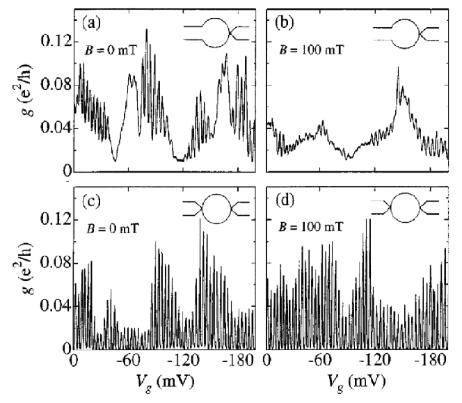
Figure 24: Conductance showing Coulomb blockade oscillations as a function of gate voltage $V_{g}$ in the open-channel regime [(a), (b)] and weak-tunneling regime [(c), (d)] at $B=0$mT, and $B=100$mT (the crossover between the Orthogonal and Unitary ensembles occurs at $B\approx 20$mT for this quantum dot), from Ref. [154]. Note that the oscillations in the open-channel case are stronger at $B=0$mT compared to $B=100$mT, unlike the weak-tunneling Coulomb blockade.

Also note that the average conductance in the case of a symmetric weak-tunneling setup [panels (c) and (d) of Fig. 24] grows with the application of the symmetry-breaking magnetic field. This is in agreement with the low temperature RMT predictions discussed in Section 3.1, see Eqs. (140)–(142). If the two junctions to the dot are of the same average conductance, then the crossover from the Orthogonal to the Unitary ensemble should result in the increase of $\langle G_{\rm peak}\rangle$ by a factor of $4/3$ at low temperatures. More detailed measurements of the magnetic field dependence of the average peak heights were reported recently in Ref. [131].

5 Conclusions

In the beginning of this Review, see Subsections 2.1-2.3.3, we have derived the model Hamiltonian of an isolated dot. One of the main assumptions in that derivation was that the electron states are random. Randomness of the one-electron states, a large dimensionless conductance inside the dot ($g\equiv E_{T}/\Delta\gg 1$), and relative weakness of the electron-electron interaction ($r_{s}\>{{}^{{}_{\displaystyle<}}_{\displaystyle\sim}}\>1$) allowed for a relatively simple description of an isolated dot. The main part of the Hamiltonian of the dot is universal; it consists of a free-electron part described by Random Matrix Theory and an interaction term, which is not random, see Eq. (93). Corrections to this universal part of the Hamiltonian are small at $g\gg 1$. In the discussion of the transport phenomena and of other effects which result from the contact of the dot with external electron reservoirs (leads), we have considered that universal part of the Hamiltonian only. Despite this extremely simple description of the physics inside the quantum dot, a large variety of intricate physical effects is uncovered when the dot is coupled to the outside world via point contacts. These effects range from quantum interference transport phenomena in the regime strong Coulomb blockade (Subsections 3.1 and 3.2) to the effects of quantum charge fluctuations and non-Fermi liquid behavior of partially open quantum dots (Subsection 4.4). Remarkably, the low temperature behavior of transport through a quantum dot with a finite spin is always dominated by the Kondo effect, see Subsections 3.3 and 4.3.

In this concluding Section, we will mention three areas of research on quantum effects in quantum dots that are not covered in this review.

The first area is related to the problem of electron relaxation in a constrained geometry. It is well-known that in a bulk clean Fermi liquid the relaxation rate of an electron with energy $\varepsilon$ is $1/\tau_{\varepsilon}\sim\varepsilon^{2}/E_{F}$. In a confined system, an electron occupying a discrete level with energy $\varepsilon$ can decay with the excitation of an electron-hole pair. It was shown in Ref. [155] that the relaxation rate $1/\tau_{\varepsilon}\sim\Delta\varepsilon^{2}/E_{T}^{2}$ still scales as $\propto\varepsilon^{2}$ with the electron energy. The quadratic dependence of the inelastic relaxation rate on the the electron energy reflects the smallness of the phase volume of the final state, and, therefore, is the same for the quantum dots and for the clean Fermi liquid. The proportionality coefficient is, however, much larger than its value for the clean system, which reflects the stronger correlation of one-particle states of the disordered dot in comparison with the plane waves. Nevertheless, $1/\tau_{\varepsilon}\ll\Delta$ for $\varepsilon\ll E_{T}$, which justifies the one particle approximation as the starting point for isolated quantum dot.

The treatment of Ref. [155] neglected the discreteness of the spectrum of the final states. The question of the validity of such an approach was first addressed in Ref. [67] where it was shown that the approximation of the one particle density of states by the discrete levels broadened to $\hbar/\tau_{\varepsilon}$ is correct only at energies larger than $E^{*}\simeq\sqrt{E_{T}\Delta}$. At such energies, the three particle state obtained as a result of one-particle decay will decay further into five-particle state, etc., thus resulting in a true decay, without the possibility of a return to the initial state. If the energies of the initial state is smaller than $E^{*}$, the three particle state is not strongly connected to the five particle state, so that the quantum dot will return to the original state. In that case, the level is broadened much less than it is found in Ref. [155].

Inelastic processes within the dot affect the conductance through the dot. This is exemplified in the temperature dependence of the conductance of an open quantum dot, Eq. (4.7). It follows from this formula, that the weak localization correction (second term) does not depend on temperature. This is, however, a consequence of neglecting the inelastic process within the dot. Only due to the those processes, the phase coherence inside the dot is destroyed. Quantitatively, it is described approximately [156, 157, 158] by the replacement $N_{\rm ch}^{o}+1\to N_{\rm ch}^{o}+1+2\pi/(\tau_{\varphi}\Delta)$ with $\tau_{\varphi}$ equal to the inelastic relaxation time for an electron with energy $T$. From the theory, one expects $\tau_{\varphi}\propto T^{-2}$. Experiments with open quantum dots [159] give the result $\tau_{\varphi}\propto T^{-1}$. The reasons for such discrepancy have not been identified as of yet.

The second area of research omitted in this review is related to the spin-spin interactions. These effects become significant at $r_{s}\sim 1$, and may result in a formation of a dot ground state with spin exceeding $1/2$. Sufficiently strong electron-electron interaction (large $r_{s}$) should result in a complete spin polarization (Stoner instability). However, fluctuations of the density of orbital levels may result in an anomalously large spin of a finite-size sample even at moderate values of $r_{s}$. This problem was studied in Refs. [76, 77, 78]. The simplest manifestation of the anomalous spin polarization is the transition from a singlet to triplet state in a dot when the number of electrons is even. Such a transition can be achieved by a decrease of the spacing between the doubly-occupied level and the next empty orbital state. In very small quantum dots, the level separation can be controlled experimentally by application of a magnetic field that affects the electron orbital motion [160]. The singlet-triplet transition can be seen experimentally in a measurement of the conductance through the dot [161] as it results in the increase of Kondo temperature at the transition point [162, 163]. In larger dots, it can also be seen by the parametric dependence of Coulomb blockade peaks on the magnetic field, which shows a kink at the single-triplet transition [77], or a change in the peak-to-peak correlations from neighboring peaks to next-neighboring peaks [164]. Sofar, the effect of the anomalous spin polarization on the conductance was considered only in the regime of weak tunneling. The counterpart of this effect for the strong tunneling regime has not been studied.

Finally, we have not discussed the effects of a time-dependent change of the shape of the dot by external gates; this effect is described by the first term in Eq. (93). We mention here only the suppression of the weak localization correction in quantum dots and generation of a dc-current by a time depenedent perturbation [165, 166, 167, 168, 169].

Appendices

Appendix A Correlation of the wave-functions in ballistic dots.

Consider a system confined by a potential $U(\vec{r})$ that is smooth on the scale $a$ much larger than the Fermi wavelength. The Hamiltonian function ${\cal H}(\vec{p},\vec{r})$,

$${\cal H}(\vec{p},\vec{r})=\frac{\vec{p}^{2}}{2m}+U(\vec{r}),$$ (370)

serves as a classical counterpart of the Hamiltonian of the system. The classical diffusion in space, Eq. (11) is replaced by the classical evolution on the energy shell ${\cal H}(\vec{p},\vec{r})=E_{F}$. This classical evolution is described by Perron-Frobenius equation

$$\left[\frac{\partial{\cal H}}{\partial\vec{p}}\frac{\partial}{\partial\vec{r}}-\frac{\partial{\cal H}}{\partial\vec{r}}\frac{\partial}{\partial\vec{p}}-\frac{1}{\tau}\left(\vec{n}\times\frac{\partial}{\partial\vec{n}}\right)^{2}\right]f_{m}(\vec{n},\vec{r})=\gamma_{m}f_{m}(\vec{n},\vec{r}),$$ (371)

where $\vec{n}$ is the unit vector in the momentum direction. The last term on the left hand side of Eq. (370) is necessary for the regularization of the otherwise singular eigenfunctions of the Perron-Frobenius operator. The calculation of the quantum corrections (e.g., weak localization) to the chaotic dynamics requires a finite value of $1/\tau\simeq\hbar/(ma^{2})$, [157, 170], however, for the leading in $1/g$ approximation the limit ${\tau}\to\infty$ should be taken only in the end of the calculation.

The normalization condition (48) is replaced with

$$\int d\vec{r}d\vec{n}f_{m}(\vec{n},\vec{r})f_{m^{\prime}}(-\vec{n},\vec{r})=\Omega_{d}\delta_{mm^{\prime}},$$ (372)

where $\Omega_{d}$ is the surface area of the unit sphere in $d$-dimensional space, $\Omega_{2}=2\pi$, $\Omega_{3}=4\pi$.

The product of two Green functions, compare with Eq. (47), averaged over energy is given by, see e.g. Ref. [157],

$$\langle{\cal G}^{R}(\varepsilon+\omega;\vec{r}_{1}^{+},\vec{r}_{2}^{-}){\cal G}^{A}(\varepsilon;\vec{r}_{1}^{-},\vec{r}_{2}^{+})\rangle$$ (373)

$$\quad=\frac{2\pi}{\Delta{\cal V}_{d}}\sum_{\gamma_{m}}\int\frac{d\vec{n}_{1}}{\Omega_{d}}\frac{d\vec{n}_{2}}{\Omega_{d}}e^{ik_{F}\vec{n}_{1}\vec{r}_{1}}e^{ik_{F}\vec{n}_{2}\vec{r}_{2}}\frac{f_{m}(\vec{n}_{1},\vec{R}_{1})f_{m}(\vec{n}_{2},\vec{R}_{2})}{\left(-i\omega+\gamma_{m}\right)},$$

$$\quad\vec{r}_{1,2}^{\pm}=\vec{R}_{1,2}\pm\frac{\vec{r}_{1,2}}{2}.$$

Repeating all the steps in the derivation of Eq. (50) from Eq. (39) we obtain instead of Eq. (50)

$$\langle H_{\alpha\beta\gamma\delta}^{(1/g)}\rangle=c_{1}\lambda\frac{\Delta}{g}\left(\delta_{\alpha\delta}\delta_{\beta\gamma}+\delta_{\alpha\gamma}\delta_{\beta\delta}\right);$$ (374)

$$c_{1}=\lim_{\delta r\to+0}\frac{1}{\pi}\sum_{\gamma_{m}\neq 0}\left[\frac{{\rm Re}\gamma_{1}}{\gamma_{m}}\int\frac{d\vec{n}_{1}}{\Omega_{d}}\frac{d\vec{n}_{2}}{\Omega_{d}}\int d\vec{r}f_{m}(\vec{n}_{1},\vec{r}-\vec{n}_{1}\delta r)f_{m}(\vec{n}_{2},\vec{r})\right],$$

where the dimensionless conductance of the dot $g$ is defined similarly to Eq. (15),

$$g=\frac{{\rm Re}\gamma_{1}}{\Delta}.$$

It is important to emphasize that, unlike in the diffusive case, the expression for the matrix element involves also the eigenfunctions of the classical evolution operator. This can be traced to the difference of the normaliztion conditions (48) and (372).

Analogously, Eq. (51) acquires the form,

$$\langle\left[\delta H_{\alpha\beta\gamma\delta}^{(1/g)}\right]^{2}\rangle=c_{2}\lambda^{2}\left(\frac{\Delta}{g}\right)^{2},$$ (375)

$$c_{2}=\frac{2}{\pi^{2}}\lim_{\delta r\to+0}\sum_{\gamma_{m},\gamma_{m\prime}\neq 0}\Bigg{[}\left(\frac{{\rm Re}\gamma_{1}}{\gamma_{m}}\right)\left(\frac{{\rm Re}\gamma_{1}}{\gamma_{m\prime}}\right)\int\frac{d\vec{n}_{1}}{\Omega_{d}}\frac{d\vec{n}_{2}}{\Omega_{d}}\frac{d\vec{n}_{3}}{\Omega_{d}}\frac{d\vec{n}_{4}}{\Omega_{d}}$$

$$\hphantom{c_{2}=}\mbox{}\times\int d\vec{r}_{1}d\vec{r}_{2}f_{m}(\vec{n}_{1},\vec{r}_{1}-\vec{n}_{1}\delta r)f_{m}(\vec{n}_{2},\vec{r}_{2})f_{m\prime}(\vec{n}_{3},\vec{r}_{2}-\vec{n}_{3}\delta r)f_{m\prime}(\vec{n}_{2},\vec{r}_{1})\Bigg{]}.$$

Appendix B Effect of the Interaction in the Cooper channel

As we already emphasized in Sec. 2.3, the universal description of the interaction by Hamiltonian (35) is valid provided that the coupling constants in this Hamiltonian are calculated with taking into account virtual transitions to the excited states which are beyond the energy strip in which the Hamiltonian (35) is defined. For a weak short range interaction, these transitions only insignificantly change the interaction constants $E_{c}$ and $J_{S}$ for the charge and spin channels, respectively. The situation is different for the Cooper channel, where the renormalization is significant even for a weak interaction.

Consider the lowest order perturbation theory correction to the interaction matrix element $\delta M_{\alpha\alpha\beta\beta}$ shown in Fig. 25a.

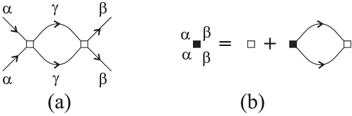
Figure 25: Diagrammatic expansion for the renormalization of the matrix elements in the Cooper channel: (a) The first order correction; (b) summation of the leading logarithm series for the renormalized coupling constant. Intermediate states $\gamma$ are only those lying outside the energy strip $E_{T}$.

The analytic expression for this correction is

$$\delta{\cal H}_{\alpha\alpha\beta\beta}\approx-\sum_{|\varepsilon_{\gamma,\delta}|>E_{T}}\frac{{\cal H}_{\alpha\alpha\gamma\delta}{\cal H}_{\delta\gamma\beta\beta}}{|\varepsilon_{\gamma}+\varepsilon_{\delta}|}\theta(\varepsilon_{\gamma}\varepsilon_{\delta}).$$ (376)

According to the structure of the matrix elements discussed in Sec. 2.3.1, the largest contribution comes from the terms with $\gamma=\delta$, and one finds

$$\delta{\cal H}_{\alpha\alpha\beta\beta}\approx-\Delta^{-1}\langle{\cal H}_{\alpha\alpha\beta\beta}\rangle^{2}\ln\left(\frac{\varepsilon^{*}}{E_{T}}\right),$$

where $\varepsilon^{*}$ is a high energy cut-off above which the approximation of the instantaneous interaction and equidistant spectrum becomes non-applicable. Because of the large logarithmic factor here, the renormalization of the coupling constants in the Cooper channel is significant, even if the interaction is weak, $\langle{\cal H}_{\alpha\alpha\beta\beta}\rangle\ll\Delta$.

To take into account this renormalization, one has to sum the leading logarithmically divergent series shown in Fig. 25 b. This results in the renormalization of the interaction constant in comparison with its bare value,

$$J_{c}\to\tilde{J}_{c}=\frac{J_{c}}{1+\frac{J_{c}}{\Delta}\ln\left(\frac{\varepsilon^{*}}{E_{T}}\right)}.$$ (377)

One can see, that for repulsive interaction, $J_{c}>0$, the effective interaction in the Cooper channel is always weak, and for the majority of effects it can be neglected form the very beginning. For the attractive interaction, $J_{c}<0$, the interaction constant renormalizes to strong coupling limit and diverges at the energy scale $\Delta_{c}=\varepsilon^{*}e^{-\Delta/|J_{c}|}$, which is nothing but the superconducting gap in BCS theory. If the inequaltiy $\Delta_{c}<E_{T}$ holds, one can still use Eq. (35) for the description of low-energy physics of a dot; in particular, effects of finite level spacing on superconductivity can be accounted for in the formalism described here. On the other hand, if $\Delta_{c}>E_{T}$, the random matrix description for the interaction effects is not applicable.

Appendix C Scattering states and derivation of Eq. (99)

In this appendix we discuss the precise definitions of the scattering states $\psi_{j}(k)$ in the lead Hamiltonian $H_{L}$ of Eq. (96) and the derivation of the relation (99) between the scattering matrix $S$ and the matrices $W$, $H$, and $U$ parameterizing the Hamiltonian of the dot-lead system. Our discussion follows that of Refs. [86, 88, 89, 90, 91].

Figure 26: Schematic picture of the dot with one of the leads.

We illustrate a part of the Hamiltonian (96) corresponding to one of the leads in Fig 26. For each particular lead, we take the direction towards the dot as positive $x$, and locate the lead-dot interface near $x=0$. The electron operators then take the form

$$\hat{\psi}_{e}(\vec{r})=\sum_{j=1}^{N_{\rm ch}}\Phi_{j}(\vec{r}_{\perp})\sum_{l=1}^{N_{\rm ch}}\int\frac{dk}{2\pi}\left[U_{jl}^{*}\,e^{i(k_{F}+k)x}+U_{jl}^{\vphantom{nothing}}\,e^{-i(k_{F}+k)x}\right]\hat{\psi}_{j}(k),$$ (378)

where $\Phi_{j}(\vec{r}_{\perp})$ characterizes the structure of the wave function in the transverse direction. The unitary matrix $U_{jl}$ describes the scattering in the absence of any coupling to the quantum dot [86, 91]. If the contact between the lead and the dot is defined as in Fig. 26, with Dirichlet boundary conditions at the lead-dot interface, electrons pick up a phase shift $\pi$ at the lead-dot interface at $x=0$, but otherwise remain in the same transverse mode, hence $U_{jl}=i\delta_{jl}$ in that case.

In the absence of electron-electron interactions in the dot, the wave function in the leads at the energy $\varepsilon=v_{F}k$ acquires the form

$${\psi}_{e}(\vec{r})=\sum_{j}\Phi_{j}(\vec{r}_{\perp})\left[a_{j}^{\rm in}e^{i\left(k_{F}+\varepsilon/v_{F}\right)x}+a_{j}^{\rm out}e^{-i\left(k_{F}+\varepsilon/v_{F}\right)x}\right].$$ (379)

The amplitudes of the out-going waves $a_{j}^{\rm out}$ are related to the amplitudes of in-going waves $a_{j}^{\rm in}$ by the $N_{\rm ch}\times N_{\rm ch}$ scattering matrix $S(\varepsilon)$,

$$a_{i}^{\rm out}=\sum_{j=1}^{N_{\rm ch}}S_{ij}(\varepsilon)a_{j}^{\rm in}.$$ (380)

The matrix $S$ is unitary, as required by particle conservation. In order to express the scattering matrix $S$ in terms of the Hamitonian of the closed dot, the coupling matrix $W$ and the unitary matrix $U$, we represent the Hamiltonian (95) in terms of a Schrödinger equation for the wavefunction $\psi_{j}(x)$, which corresponds to the Fourier transform of the fermion fields $\hat{\psi}(k)$ over the entire real axis,

$$\hat{\psi}_{j}(x)=\int{dk\over 2\pi}\hat{\psi}_{j}(k)e^{-ikx},\ \ j=1,\ldots,N_{\rm ch}.$$ (381)

The operator $\hat{\psi}_{j}(x)$ is a mathematical construction that is related, but not identical to the true electron operator $\hat{\psi}_{e}(\vec{r})$ defined in Eq. (378). Then, denoting the wavefunction inside the dot as $\phi_{\mu}$, we find from Eqs. (92) and (95)–(97), that the Schrödinger equation for the entire system reads

$$\varepsilon\psi_{j}(x) = iv_{F}{\partial\psi_{j}(x)\over\partial x}+\sum_{\nu=1}^{M}W_{\nu j}^{*}\delta(x)\phi_{\nu},$$

$$\varepsilon\phi_{\mu} = \sum_{\nu=1}^{M}{\cal H}_{\mu\nu}\phi_{\nu}+\sum_{l=1}^{N_{\rm ch}}W_{\mu l}\psi_{l}(0).$$ (382)

For $x\neq 0$, Eq. (382) corresponds to a left moving particle at velocity $v_{F}$. To find the scattering matrix $S_{jl}$, we set, cf. Eq. (379),

$$\psi_{j}(x)=\left\{\begin{array}[]{ll}\displaystyle e^{-ikx}\sum_{l=1}^{N_{\rm ch}}U_{jl}^{\vphantom{nothing}}\,a^{\rm in}_{l},&\ \ \ \ x>0,\\ \displaystyle e^{-ikx}\sum_{l=1}^{N_{\rm ch}}U_{jl}^{*}\,a^{\rm out}_{l},&\ \ \ \ x<0,\end{array}\right.$$ (383)

where $k=\varepsilon/v_{F}$. At $x=0$ we use the standard regularization $\psi_{j}(0)=[\psi_{j}(-0)+\psi_{j}(+0)]/2$. Substitution of Eq. (383) into the Schrödinger equation (382) yields

$$\varepsilon\phi_{\mu} = \sum_{\nu}H_{\mu\nu}\phi_{\nu}+{\textstyle{1\over 2}}\sum_{j,l=1}^{N_{\rm ch}}W_{\mu j}(U_{jl}^{\vphantom{nothing}}a_{l}^{\rm in}+U_{jl}^{*}a_{l}^{\rm out}),$$

$$0 = iv_{F}(U_{jl}^{\vphantom{nothing}}a_{l}^{\rm in}-U_{jl}^{*}a_{l}^{\rm out})+\sum_{\nu}W_{\nu j}^{*}\phi_{\nu}.$$

The wavefunction $\phi_{\mu}$ of the dot can be eliminated from this equation, resulting in the condition (380) for the amplitudes $a^{\rm in}_{j}$ and $a^{\rm out}_{j}$, with the $N_{\rm ch}\times N_{\rm ch}$ matrix $S$ given by

$$S(\varepsilon)=U\left[1-2\pi i\nu W^{\dagger}\left({\varepsilon-{\cal H}+i\pi\nu WW^{\dagger}}\right)^{-1}W\right]U^{\rm T}.$$

This is Eq. (99) of the main text.

The coupling matrix $W$ can be represented in the form

$$W=\sqrt{\frac{\Delta M}{\pi^{2}\nu}}VO\tilde{W},$$ (384)

where $V$ is an orthogonal $M\times M$ matrix, $\tilde{W}$ is a real $N_{\rm ch}\times N_{\rm ch}$ matrix, and $O$ is an $M\times N_{\rm ch}$ projection matrix, $O_{\alpha j}=\delta_{\alpha j}$, $\alpha=1,\ldots,M$ and $j=1,\ldots,N_{\rm ch}$. The first factor in Eq. (384) ensures a convenient normalization of the matrix $\tilde{W}$. Because the distribution function of the random matrix ${\cal H}$ is invariant under rotations ${\cal H}\to V{\cal H}V^{\dagger}$, the matrix $V$ in Eq. (384) can be omitted. The matrix $\tilde{W}$ can be related to the $(2N_{\rm ch})\times(2N_{\rm ch})$ scattering matrix $S_{c}$ of the point contacts between the lead and the dot. Unlike the scattering matrix $S(\varepsilon)$ which connects the incoming and outgoing states for the entire device, the matrix $S_{c}$ characterizes the properties of each point contact connecting a lead to the dot separately. The corresponding transmission and reflection amplitudes are defined in $N_{\rm ch}\times N_{\rm ch}$ matrices $r_{c}$, $r^{\prime}_{c}$, and $t_{c}$,

$$S_{c}=\left(\matrix{r_{c}\quad&t^{\rm T}_{c}\cr t_{c}\quad&r^{\prime}_{c}}\right),$$ (385)

which can be expressed [92] in terms of the coupling matrix $\tilde{W}$ and the matrix $U$ of Eq. (378),

$$r_{c} = U\frac{1-\tilde{W}^{\dagger}\tilde{W}}{1+\tilde{W}^{\dagger}\tilde{W}}U^{\rm T},\quad r_{c}^{\prime}=-\tilde{W}\frac{1-\tilde{W}^{\dagger}\tilde{W}}{1+\tilde{W}^{\dagger}\tilde{W}}{\tilde{W}}^{-1},\quad t_{c}=\tilde{W}\frac{2}{1+\tilde{W}^{\dagger}\tilde{W}}U.$$

The matrix $r_{c}$ expresses the reflection from a point contact to the leads, $r_{c}^{\prime}$ corresponds to the reflection of an electron entering the point contact from the dot, and the matrix $t_{c}$ describes the transmission through the point contact from a lead to the dot. A contact is called ideal if $r_{c}=r_{c}^{\prime}=0$, or, equivalently, $\tilde{W}^{\dagger}\tilde{W}=1$.

Appendix D Mesoscopic fluctuations of elastic co-tunneling far from the peaks

The calculation of the magnetic field dependence of the mesoscopic fluctuations of elastic co-tunneling is more complicated than in the pure orthogonal and unitary ensembles, as in the crossover between the orthogonal and unitary ensembles the electron and hole amplitudes become correlated. This is because the wavefunctions for different energies are not independent in the crossover regime. The corresponding correlation functions are obtained from Eqs. (151) and (25),

$$\langle F_{e}F_{h}^{\ast}\rangle=\frac{\Delta}{E_{e}+E_{h}}\left[\Lambda_{1}\left(\frac{N_{h}^{D}\Delta}{2\pi E_{h}},1+\frac{E_{h}}{E_{e}}\right)+\Lambda_{1}\left(\frac{N_{h}^{D}\Delta}{2\pi E_{h}},1+\frac{E_{e}}{E_{h}}\right)\right],$$ (387)

$$\langle F_{e}F_{h}\rangle=\frac{\Delta}{E_{e}+E_{h}}\left[\Lambda_{1}\left(\frac{N_{h}^{C}\Delta}{2\pi E_{h}},1+\frac{E_{h}}{E_{e}}\right)+\Lambda_{1}\left(\frac{N_{h}^{C}\Delta}{2\pi E_{h}},1+\frac{E_{e}}{E_{h}}\right)\right],$$

where the dimensionless functions $\Lambda_{1}(x)$ is given by

$$\Lambda_{1}(x,y) = \frac{1}{\pi\left(1+x^{2}\right)}\left\{\frac{\pi^{2}x}{6}+\left(-\frac{\pi x}{2}+\ln xy\right)\arctan xy-x{\mathrm{L}i}_{2}(1-y)\right.$$

$$-\left.\frac{1}{2}\left(x\ln x+x+\frac{\pi}{2}\right)\ln\left(1+x^{2}y^{2}\right)-{\mathrm{R}e}\left[(i+x){\mathrm{L}i}_{2}(-ixy)\right]\right\},$$

with ${\mathrm{L}i}_{2}(x)$ being the second polylogarithm function [103]. The asymptotic behavior of functions $\Lambda_{1}$ is $\Lambda_{1}(x,y)=(xy/\pi)\ln(xy)$ for $x\ll 1$, and $\Lambda_{1}(x,y)=\left[\frac{1}{2}\ln^{2}(xy)-\ln^{2}x\right]/(\pi x)$ for $x\gg 1$. The limits of the pure orthogonal (unitary) ensembles (153) are recovered by putting $N_{h}^{D}=0$ and $N_{h}^{C}=0(\infty)$ in Eq. (387).

The correlation function of the conductances at different values of the magnetic field is somewhat involved,

$$\frac{\langle\delta G(B_{1})\delta G(B_{2})\rangle}{\langle G\rangle^{2}} = \left\{\frac{E_{h}}{E_{e}+E_{h}}\Lambda\left(\frac{N_{h}^{D}\Delta}{2\pi E_{e}}\right)\right.$$

$$\mbox{}+\left.\frac{E_{h}E_{e}}{\left(E_{e}+E_{h}\right)^{2}}\Lambda_{1}\left(\frac{N_{h}^{D}\Delta}{2\pi E_{h}},1+\frac{E_{h}}{E_{e}}\right)+E_{e}\leftrightarrow E_{h}\right\}^{2}$$

$$\mbox{}+N_{h}^{D}\leftrightarrow N_{h}^{C}.$$

In this general case, where the gate voltage can be anywhere in the Coulomb blockade valley, it is impossible to point out the single scale for the magnetic field. However, in the vicinity of the peaks, $E_{e}\gg E_{h}$ or $E_{e}\ll E_{h}$, the situation simplifies significantly, and one obtains the universal dependence (162).

The dependence of the crossover parameter $\lambda$ from Eq. (164) on the magnetic flux $\Phi$ in our case is

$$\lambda = \left\{\frac{E_{h}}{E_{e}+E_{h}}\Lambda\left(\frac{N_{h}^{C}\Delta}{2\pi E_{e}}\right)+\frac{E_{h}E_{e}}{\left(E_{e}+E_{h}\right)^{2}}\Lambda_{1}\left(\frac{N_{h}^{C}\Delta}{2\pi E_{h}},1+\frac{E_{h}}{E_{e}}\right)\right.$$ (390)

$$\left.\vphantom{\left(\frac{N_{h}^{C}\Delta}{2\pi E_{e}}\right)}\mbox{}+E_{e}\leftrightarrow E_{h}\right\},$$

where the functions $\Lambda$, $\Lambda_{1}$ are defined in Eqs. (161) and (LABEL:eq:a2.2), and $N_{h}^{C}$ is defined in Eq. (20) with $\Phi_{1}=\Phi_{2}=\Phi$. As before, there is no universal dependence on the magnetic field. In the vicinity of the peak, however, we recover the universal result (165).

Appendix E Derivation of the Hamiltonian (240)

To include the second junction we should modify Hamiltonian given in Eqs. (209), (211) and (214): in the charging energy, Eq. (211), the variable $\theta_{\rho}(0)$ should be replaced by the difference $\theta_{\rho}(0)-\theta_{\rho}(L)$; we should also return from Eq. (214) to the generic form (208) of the free-field Hamiltonian, and replace the boundary condition Eq. (215) by a barrier described by the Hamiltonian

$$\hat{H}_{r1}=-\frac{2}{\pi}|r_{1}|D\cos[2\sqrt{\pi}\theta_{\rho}(L)]\cos[2\sqrt{\pi}\theta_{s}(L)],\\$$ (391)

which is similar to Eq. (209). Similar to the one-junction case [cf. Eq. (213)], in the energy range $E\ll E_{c}$ the fluctuations involving the total charge of the dot are pinned,

$$\frac{2e}{\sqrt{\pi}}\langle[\theta_{\rho}(0)-\theta_{\rho}(L)]\rangle_{q}=e{\cal N},$$ (392)

and fluctuations of the field $\theta_{\rho}$ have the same phase at both junctions. If, on the other hand, $E\gg\Delta$, this is the only constraint on the fluctuations of the charge and spin fields at two different junctions. Therefore, in the energy domain $E_{c}\gg E\gg\Delta$, there are three independent modes left: the spin modes $\theta_{s}$ and $\theta_{s1}$ at each of the junctions, and one charge mode $\tilde{\theta}_{\rho}$ corresponding to passing of the charge across the entire dot. It is more compact to describe the system in terms of the effective action [140], rather than a Hamiltonian,

$$S = \sum_{i\omega_{n}}|\omega_{n}|\left[4|\tilde{\theta}_{\rho}(\omega_{n})|^{2}+2|\theta_{s}(\omega_{n})|^{2}+2|\theta_{s1}(\omega_{n})|^{2}\right]$$ (393)

$$+ 4\left[\frac{e^{-{\bf C}}}{\pi^{3}}E_{c}D\right]^{\frac{1}{2}}\int d\tau\left\{|r|\cos[\pi{\cal N}-2\sqrt{\pi}\tilde{\theta}_{\rho}(\tau)]\cos[2\sqrt{\pi}\theta_{s}(\tau)]\right.$$

$$+ \left.|r_{1}|\cos[2\sqrt{\pi}\tilde{\theta}_{\rho}(\tau)]\cos[2\sqrt{\pi}\theta_{s1}(\tau)]\right\},$$

here $\tau$ is the imaginary time, and $\omega_{n}$ is the Matsubara frequency. The spin degrees of freedom at each junction are described by $g=1/2$ Luttinger liquids, and the mode corresponding to the remaining charge degree of freedom, is a Luttinger liquid with $g=1/4$; its increased stiffness comes from the low-energy constraint Eq. (392) of the charge neutrality of the dot. It is easy to check that because of this increased stiffness [i. e., because of ($g<1/2$)], the reflection at the point contacts is a relevant perturbation. If the bare reflection amplitudes $|r|$ and $|r_{1}|$ are small, then with the reduction of the energy scale $E$ they grow as $(E_{c}/E)^{1/4}$, independently of each other. We intend to consider the asymmetric geometry: the bare reflection amplitudes are very different: $|r|\ll|r_{1}|$. Then, the crossover to weak tunneling through the $x=L$ junction is either occurs upon reaching the energy scale $\sim E_{c}|r_{1}|^{4}$, or tunneling is weak from the very beginning. At energies $E\>{{}^{{}_{\displaystyle<}}_{\displaystyle\sim}}\>E_{c}|r_{1}|^{4}$, the variables $\theta_{s1}$ and $\tilde{\theta}_{\rho}$ are fixed most of the time, so that $\cos(2\sqrt{\pi}\tilde{\theta}_{\rho})\cos(2\sqrt{\pi}\theta_{s1})=1$, to ensure the energy minimum of the junction. The system makes rare hops between various configurations satisfying the energy minimum condition. Upon further reduction of the band width, the effective backscattering at $x=0$ follows the renormalization prescribed by Eq. (222), and reaches the limit of the weak tunneling at energies $\sim E_{c}|r_{1}r\cos\pi{\cal N}|^{2}$. This energy scale coincides with Eq. (223) if $|r_{1}|\sim 1$, and replaces it if $|r_{1}|$ is small. Note that similar to the condition (227), the spatial quantization of the electron states in the dot does not affect the crossover to the regime of weak tunneling, if $\Delta\ll E_{c}|r_{1}r\cos\pi{\cal N}|^{2}$. In that regime, the system performs rare hops between the minima of the “potential”

$$U\{\theta_{s},\theta_{s1},\tilde{\theta}_{\rho}\}= - {\cal U}\cos(\pi{\cal N}-2\sqrt{\pi}\tilde{\theta}_{\rho})\cos(2\sqrt{\pi}\theta_{s})$$ (394)

$$- {\cal U}_{1}\cos(2\sqrt{\pi}\tilde{\theta}_{\rho})\cos(2\sqrt{\pi}\theta_{s1}),$$

represented by the last two lines in the action (393). [Here the renormalization-dependent energies ${\cal U}>0$ and ${\cal U}_{1}>0$ replace the corresponding bare values entering in Eq. (393).] In the minima of the potential (394), the spin of the dot $(\sqrt{\pi}/2)(\theta_{s}-\theta_{s1})$ is integer or half-integer, depending on the value of ${\cal N}$, cf. Eq. (4.2). There are three types of hops which connect the minima of the potential (394). Two of the types, $\theta_{s}(0)\to\theta_{s}(0)\pm\sqrt{\pi}$ and $\theta_{s1}(0)\to\theta_{s1}(0)\pm\sqrt{\pi}$, are already familiar to us from the single-junction case, see Equation (228) and the discussion which follows that Equation. These hops correspond to a change by $1$ of the $z$-projection of the dot’s spin via spin exchange with one of the leads. The third type of hops involves a simultaneous change of all three fields:

$$\theta_{s}(0)\to\theta_{s}(0)\pm\sqrt{\pi}/2,\,\,\,\theta_{s1}(0)\to\theta_{s1}(0)\pm\sqrt{\pi}/2,\,\,\,\tilde{\theta}_{\rho}(0)\to\tilde{\theta}_{\rho}(0)\pm\sqrt{\pi}/2.$$

In such a hop, one electron (charge $e$ and spin $s_{z}=\pm 1/2$) is transferred across the dot; the spin of this electron and the dot’s spin may flip in this process. The corresponding tunneling Hamiltonian,

$$\hat{H}^{0L}_{\pm}\propto-\cos\left(\!\frac{\sqrt{\pi}}{2}\tilde{\phi}_{\rho}^{\pm}\!\right)\cos\left(\!\frac{\sqrt{\pi}}{2}\phi_{s1}^{\pm}\!\right)\cos\left(\!\frac{\sqrt{\pi}}{2}\phi_{s}^{\pm}\!\right),$$ (395)

supplements Eq. (228) and a similar equation for the $x=L$ junction,

$$\hat{H}^{L}_{\pm}\propto-\cos\left\{\sqrt{\pi}[\phi_{s1}(+0)-\phi_{s1}(-0)]\right\}.$$ (396)

Here $\phi_{s1}^{\pm}=\phi_{s1}(x=L+0)-\phi_{s1}(x=L-0)$ and $\tilde{\phi}_{\rho}^{\pm}=\tilde{\phi}_{\rho}(x=+0)-\tilde{\phi}_{\rho}(x=-0)$ are the discontinuities of the respective fields at the junction (for the field $\tilde{\phi}_{\rho}$ the discontinuity is the same at both junctions). All three Hamiltonians, Eqs. (395), (396) and Eq. (228), have the same scaling exponent, as can be easily checked with the help of the action (393). These three Hamiltonians represent the easy-plane part of the exchange interaction. The $SU(2)$ symmetry guarantees the existence of terms like Eq. (229), which restore the isotropy of the exchange. The exchange interaction changes the spin of the dot by an integer. If we account for the finite level spacing, then the lowest energy states would correspond to the smallest possible spin of the dot, like in the one-junction geometry considered above. Kondo effect develops only if the spin of the dot is $1/2$. This doublet state is realized in the dot periodically with the gate voltage, when $\cos\pi{\cal N}<0$ (we assume here $|r_{1}|\gg|r|$). In Subsection 4.3) we concentrate on the doublet state only. Returning to the fermionic variables at $E\ll E_{c}|r_{1}r\cos\pi{\cal N}|^{2}$, we find the exchange Hamiltonian (240) which generalizes Eq. (230) to the case of two junctions.

Appendix F Canonical versus grand canonical ensembles

A crucial step in the effective action formalism is the redefinition (256) of the charge operator $\hat{n}$ in terms of the fermion operators in the leads. As was discussed below Eq. (256), strictly speaking, such a redefinition requires a canonical description of the entire system, i.e., that the total number of particles in the leads and the quantum dot is kept fixed in the ensemble. A grand-canonical approach, as in Sec. 4.5.1, can be used only when all observables are considered at a single value of the gate voltage ${\cal N}$, or when physical observables are a periodic function of ${\cal N}$. For a non-periodic ${\cal N}$-dependence (i.e., for mesoscopic fluctuations of the differential capacitance), a canonical description has to be used. In this section, we discuss implementation of the canonical constraint in the grand-canonical theory. In particular, we show, within the effective action formalism, that for $T\gg N_{\rm ch}\Delta$ or $N_{\rm ch}\gg 1$, the canonical constraint can be accounted for in the grand-canonical description by the dependence (328) of the chemical potential $\mu$ on the gate voltage ${\cal N}$.

To go between the canonical and grand-canonical descriptions, we use the inverse Laplace transform that relates the thermodynamic potential $\Omega_{N_{p}}$ in a canonical ensemble with $N_{p}$ particles to the thermodynamical potential $\Omega(\mu)$ in a grand-canonical ensemble with chemical potential $\mu$,

$$e^{-\Omega_{N_{p}}/T}=\mbox{Tr}_{N_{p}}\,e^{-\hat{H}/T} = \int_{-\pi Ti}^{\pi Ti}\frac{d\mu}{2\pi iT}\,\mbox{Tr}\,e^{-(\hat{H}-\mu\hat{N_{p}})/T}e^{\mu N_{p}/T}$$ (397)

Here $\mbox{Tr}_{N_{p}}$ denotes a trace over all states with a fixed number of particles $N_{p}$, Tr  is a trace over all states with all numbers of particles, and $\hat{N}_{p}$ is the operator for the total number of particles.

Hence, what we need is the dependence of $\Omega$ on a complex chemical potential $\mu$ in a strip $\pi T<\mbox{Im}\,\mu<\pi T$. The modification of the effective action theory of Sec. 4.5.1 to include a complex chemical potential is straightforward, because all intermediate steps are analytic in $\mu$ for $\pi T<\mbox{Im}\,\mu<\pi T$. In the final result, the $\mu$-dependence appears through the $\mu$-dependence of the scattering matrix, $S(\mu,t)\to S(0,t)e^{-i\mu t}$ and through the $\mu$-dependence of the thermodynamic potential of the lead. To find the latter, we include $\mu$ into the charging energy,

$$\hat{H}_{\rm eff}-\mu{\hat{N}}_{p,L} = iv_{F}\sum_{j}\int_{-\infty}^{\infty}dx\left(\hat{\psi}^{\dagger}_{L,j}\partial_{x}\hat{\psi}_{L,j}-\hat{\psi}^{\dagger}_{R,j}\partial_{x}\hat{\psi}_{R,j}\right)$$ (398)

$$\mbox{}+{E_{c}}\left(\sum_{j}\int_{-\infty}^{0}dx:\hat{\psi}^{\dagger}_{L,j}\hat{\psi}_{L,j}+\hat{\psi}^{\dagger}_{R,j}\hat{\psi}_{R,j}:+{\cal N}^{\prime}\right)^{2}$$

$$\mbox{}-{\mu^{2}\over 4E_{c}}-\mu{\cal N}-\mu\langle{\hat{N}}_{p,L}\rangle_{q},$$

where ${\cal N}^{\prime}={\cal N}+\mu/(2E_{c})$ and ${\hat{N}}_{p,L}$ is the number of particles in the leads. Hence, by the second line of Eq. (398), wherever we found an explicit ${\cal N}$-dependence, ${\cal N}$ should be replaced by ${\cal N}+\mu/(2E_{c})$. The term $\mu\langle\hat{N}_{p,L}\rangle_{q}$ denotes the quantum mechanical average of the number of particles in the lead and arises due to the normal ordering of the $\hat{\psi}$-fields.

Let us now discuss the implication of this scheme for the calculation of the mesoscopic fluctuations of the differential capacitance, that were the subject of the Subsection “Non-periodic interaction corrections to the capacitance, $K_{\mu}(s)$”. Using Eq. (334) and upon inclusion of the $\mu$-dependent contributions to $\Omega$ from Eq. (398) and the $\mu$-dependence of the scattering matrix, we find that the $\mu$-dependence of the thermodynamic potential of the entire system is given by

$$\Omega(\mu) = \Omega(0)-{\mu^{2}\over 4E_{c}}-\mu{\cal N}-\mu\langle N_{p}\rangle$$ (399)

$$\mbox{}-T\int_{0}^{\infty}dt\int_{0}^{\infty}dt^{\prime}{(t+t^{\prime})[1-i\mu(t-t^{\prime})-e^{-i\mu(t-t^{\prime})}]\mbox{Tr}\,S^{\dagger}(t^{\prime})S(t)\over 4(t-t^{\prime})\sinh[\pi T(t-t^{\prime})]}$$

$$\mbox{}+{1\over 2}{T^{2}}\sin{\pi\over N_{\rm ch}}\int_{0}^{\infty}dt\int_{0}^{\infty}dt^{\prime}\int_{t_{0}}^{\infty}ds{\mbox{Tr}\,S(t)S^{\dagger}(t^{\prime})[1-e^{-i\mu(t-t^{\prime})}]\over\sinh[\pi T(t+s)]\sinh[\pi T(t^{\prime}+s)]}$$

$$\ \ \mbox{}\times\left\{{\sinh[\pi T(s-t_{0})]\sinh[\pi T(s+t+t^{\prime}+t_{0})]\over\sinh[\pi T(t+t_{0})]\sinh[\pi T(t^{\prime}+t_{0})]}\right\}^{{1/N_{\rm ch}}},$$

where $\langle\hat{N}_{p}\rangle$ is the expectation number of the total number of particles in the system (leads and dot) at $\mu=0$. Mesoscopic fluctuations of $\Omega$ are dominated by the fluctuations of the second line in Eq. (399), which are small as $N\Delta/T$ or $1/N_{\rm ch}$ for $T\gg N\Delta$ or $N_{\rm ch}\gg 1$, respectively. Hence, to find the leading $\mu$-dependence of $\Omega(\mu)$, one can replace $\Omega$ by its ensemble average, for which one finds,

$$\langle\Omega(\mu)\rangle = \langle\Omega(0)\rangle-{\mu^{2}\over 4E_{c}}-\mu{\cal N}-\mu\langle N_{p}\rangle-{\mu^{2}\over 2\Delta}.$$ (400)

With this, the $\mu$-integration in Eq. (397) is straightforward when we choose $N_{p}=\langle{\hat{N}}_{p}\rangle$; for $T\gg N_{\rm ch}\Delta$ the integration can be done by the saddle point method and amounts to the substitution (328). Interaction and fluctuation corrections to $\Omega$ can be treated systematically by an expansion of $\exp(-\Omega/T)$ around the average (400). The differential capacitance (336) follows from Eq. (399) by twofold differentiation to ${\cal N}$.

Appendix G Correlation functions

Correlators of fermionic operators. – To complete the review of the properties of the fermionic correlation function, we give the general formulas allowing one to compute any non-vanishing average of the fermionic operators:

$$\left\langle T_{\tau}\prod_{j=1}^{N_{\rm ch}}\left[\prod_{k=1}^{n_{j}^{L}+mN_{\rm ch}}\hat{\bar{\psi}}_{L,j}(\tau_{jk}^{\bar{L}})\prod_{k=1}^{n_{j}^{L}}{\hat{\psi}}_{L,j}(\tau_{jk}^{L})\prod_{k=1}^{n_{j}^{R}}\hat{\bar{\psi}}_{R,j}(\tau_{jk}^{\bar{R}})\prod_{k=1}^{n_{j}^{R}+mN_{\rm ch}}{\hat{\psi}}_{R,j}(\tau_{jk}^{R})\right]\right\rangle_{q}=$$

$$\mbox{}\frac{1}{(2\pi v_{F})^{N_{f}}}\left(\frac{1}{f(0)t_{0}}\right)^{|m|N_{\rm ch}}e^{-i2\pi m\left({\cal N}+N_{\rm ch}/4\right)}\prod_{j=1}^{N_{\rm ch}}\left[\prod_{k>l}^{n_{j}^{L}+mN_{\rm ch}}\frac{\sin\pi T(\tau_{jk}^{\bar{L}}-\tau_{jl}^{\bar{L}})}{\pi T}\right.$$

$$\mbox{}\times\left.\prod_{k>l}^{n_{j}^{L}}\frac{\sin\pi T(\tau_{jk}^{L}-\tau_{jl}^{L})}{\pi T}\prod_{k>l}^{n_{j}^{R}}\frac{\sin\pi T(\tau_{jk}^{\bar{R}}-\tau_{jl}^{\bar{R}})}{\pi T}\prod_{k>l}^{n_{j}^{R}+mN_{\rm ch}}\frac{\sin\pi T(\tau_{jk}^{R}-\tau_{jl}^{R})}{\pi T}\right.$$

$$\mbox{}\times\left.\prod_{k=1}^{n_{j}^{L}+mN_{\rm ch}}\prod_{l=1}^{n_{j}^{L}}\frac{\pi T}{\sin\pi T(\tau_{jk}^{\bar{L}}-\tau_{jl}^{L})}\prod_{k=1}^{n_{j}^{R}}\prod_{l=1}^{n_{j}^{R}+mN_{\rm ch}}\frac{\pi T}{\sin\pi T(\tau_{jk}^{\bar{R}}-\tau_{jl}^{R})}\right]$$

$$\mbox{}\times\prod_{i,j=1}^{N_{\rm ch}}\left\{\prod_{k=1}^{n_{j}^{L}+mN_{\rm ch}}\prod_{l=1}^{n_{i}^{R}+mN_{\rm ch}}\left[f(\tau_{il}^{R}-\tau_{jk}^{\bar{L}})\right]^{1/N_{\rm ch}}\prod_{k=1}^{n_{j}^{L}}\prod_{l=1}^{n_{i}^{R}}\left[{f(\tau_{il}^{\bar{R}}-\tau_{jk}^{L})}\right]^{1/N_{\rm ch}}\right.$$

$$\mbox{}\times\left.\prod_{k=1}^{n_{j}^{L}+mN_{\rm ch}}\prod_{l=1}^{n_{i}^{R}}\left[\frac{1}{f(\tau_{il}^{\bar{R}}-\tau_{jk}^{\bar{L}})}\right]^{1/N_{\rm ch}}\prod_{k=1}^{n_{j}^{L}}\prod_{l=1}^{n_{i}^{R}+mN_{\rm ch}}\left[\frac{1}{f(\tau_{il}^{R}-\tau_{jk}^{L})}\right]^{1/N_{\rm ch}}\right\},$$

(401)

where $n_{j}^{L,R}$ are arbitrary non-negative integers, $m$ is an arbitrary integer, $N_{f}={N_{\rm ch}m+\sum_{j}(n_{j}^{L}+n_{j}^{R})}$, and we use the convention $\prod_{j=1}^{N}a_{j}=1$, for $N=0$, and $\prod_{j=1}^{N}a_{j}=0$, for $N<0$. The function $f(\tau)$ and the time scale $t_{0}$ are defined by Eq. (307). One can easily check that Eqs. (308), (309) (4.5.2) follow from Eqs. (401).

Correlators of fermionic operators and current operator. – For the calculation of the two-terminal conductance, we need correlators that involve both the fermionic operators and the current operator $I$, which is linear in the boson fields,

$$I={ev_{F}\over 2\pi}{\partial\over\partial x}\left.\sum_{j}\Lambda_{jj}\left[\hat{\varphi}_{Lj}(x)-\hat{\varphi}_{Rj}(x)\right]\right|_{x\uparrow 0},$$ (402)

Here the diagonal matrix $\Lambda$ is defined in Eq. (107). The necessary bosonic correlators are obtained from those of the free boson fields $\hat{\varphi}$ by substitution $\tau\to\tau\pm ix/v_{F}$, where the $+$ ($-$) sign is for left (right) movers. For the correlators of the current operators one thus finds

$$\langle T_{\tau}I(\tau)I(0)\rangle_{q}=\frac{1}{2\pi}\left(\frac{e^{2}}{2\pi}\right)\frac{N_{1}N_{2}}{N_{\rm ch}}\sum_{\pm}{\pi^{2}T^{2}\over\sin^{2}[\pi T(\tau\pm i0)]}.$$ (403)

The correlators of the current operators and two or four fermionic operators are most conveniently expressed in the correlators of the fermionic operators themselves,

$$\langle T_{\tau}I(\tau)I(0)\prod_{i=1}^{N_{\bar{L}}}\hat{\bar{\psi}}_{L,n_{i}}(\tau_{i}^{\bar{L}})\prod_{j=1}^{N_{{L}}}\hat{{\psi}}_{L,n_{j}}(\tau_{j}^{{L}})\prod_{k=1}^{N_{\bar{R}}}\hat{\bar{\psi}}_{R,n_{k}}(\tau_{k}^{\bar{R}})\prod_{l=1}^{N_{{R}}}\hat{{\psi}}_{R,n_{l}}(\tau_{l}^{{R}})\rangle_{q}=$$ (404)

$$\mbox{}\langle T_{\tau}I(\tau)I(0)\rangle_{q}\langle T_{\tau}\prod_{i=1}^{N_{\bar{L}}}\hat{\bar{\psi}}_{L,n_{i}}(\tau_{i}^{\bar{L}})\prod_{j=1}^{N_{{L}}}\hat{{\psi}}_{L,n_{j}}(\tau_{j}^{{L}})\prod_{k=1}^{N_{\bar{R}}}\hat{\bar{\psi}}_{R,n_{k}}(\tau_{k}^{\bar{R}})\prod_{l=1}^{N_{{R}}}\hat{{\psi}}_{R,n_{l}}(\tau_{l}^{{R}})\rangle_{q}$$

$$\mbox{}+\frac{1}{2\pi}\left(\frac{e^{2}}{2\pi}\right)\langle T_{\tau}\prod_{i=1}^{N_{\bar{L}}}\hat{\bar{\psi}}_{L,n_{i}}(\tau_{i}^{\bar{L}})\prod_{j=1}^{N_{{L}}}\hat{{\psi}}_{L,n_{j}}(\tau_{j}^{{L}})\prod_{k=1}^{N_{\bar{R}}}\hat{\bar{\psi}}_{R,n_{k}}(\tau_{k}^{\bar{R}})\prod_{l=1}^{N_{{R}}}\hat{{\psi}}_{R,n_{l}}(\tau_{l}^{{R}})\rangle_{q}$$

$$\mbox{}\times\left[\sum_{i=1}^{N_{\bar{L}}}g_{n_{i}}(\tau_{i}^{\bar{L}}-\tau)-\sum_{j=1}^{N_{{L}}}g_{n_{j}}(\tau_{j}^{{L}}-\tau)+\sum_{k=1}^{N_{\bar{R}}}g_{n_{k}}(\tau-\tau_{k}^{\bar{R}})-\sum_{l=1}^{N_{{R}}}g_{n_{l}}(\tau-\tau_{l}^{{R}})\right]$$

$$\mbox{}\times\left[\sum_{i=1}^{N_{\bar{L}}}g_{n_{i}}(\tau_{i}^{\bar{L}})-\sum_{j=1}^{N_{{L}}}g_{n_{j}}(\tau_{j}^{{L}})+\sum_{k=1}^{N_{\bar{R}}}g_{n_{k}}(-\tau_{k}^{\bar{R}})-\sum_{l=1}^{N_{{R}}}g_{n_{l}}(-\tau_{l}^{{R}})\right];$$

$$g_{n}(\tau)\equiv\Lambda_{nn}{\pi T}{\cot[\pi T(\tau+i0)]},$$

where $N_{\bar{L}},\ N_{\bar{L}},\ {N_{\bar{R}}},\ \ N_{{R}}$ are the arbitrary non-negative integers, and $n_{i}=1,\dots,N_{\rm ch}$ labels the channels. The expressions for the average of the fermionic operators were given earlier, see Eqs.  (308) – (4.5.2), and (401).

Correlators of fermionic operators and the charging operators $\hat{F}$, $\hat{F}^{\dagger}$. – Calculation of the tunneling density of states Eqs. (292) – (294) involves not only the correlation function of the fermionic operators but also the products of the operators $\hat{F},\ \hat{F}^{\dagger}$ that increase or decrease the charge of the dot by one electron. The corresponding calculation is facilitated by the observation that

$$\hat{\bar{F}}(\tau)\hat{F}(0)=e^{\hat{H}_{\rm eff}\tau}\hat{F}^{\dagger}e^{-\hat{H}_{\rm eff}\tau}\hat{F}=T_{\tau}\exp\left\{\int_{0}^{\tau}d\tau_{1}\left[\hat{H}_{\rm eff}-\hat{F}^{\dagger}\hat{H}_{\rm eff}(\tau_{1})\hat{F}\right]\right\},$$

where the one dimensional Hamiltonian is given by Eq. (295) and the commutation relation for $\hat{F},\ \hat{F}^{\dagger}$ are given by Eq. (289). In bosonized representation one finds

$$\hat{H}_{\rm eff}-\hat{F}^{\dagger}\hat{H}_{\rm eff}\hat{F} = \frac{E_{c}}{\pi}\left\{\sum_{j}\left[\hat{\varphi}_{L,j}(0)+\hat{\varphi}_{R,j}(0)\right]+2\pi\left({\cal N}-\hat{m}-1/2\right)\right\}.$$

Because this term is linear in the bosonic fields, further calculation proceeds without any difficulty with the help of Eq. (305). The operator $\hat{m}$ in Eq. (LABEL:eq:string) does not have its own dynamics and can be fixed to be any integer, $e^{i2\pi\hat{m}}=1$.

We obtain

$$\langle T_{\tau}\hat{\bar{F}}(\tau)\hat{{F}}(0)\rangle_{q}=\left|\frac{f(\tau)}{f(0)}\right|^{2/N_{\rm ch}},$$ (406)

where the dimensionless function $f(\tau)$ is defined in Eq. (306).

For the averages involving fermionic operators as well as the charge changing operators we find [compare with Eq. (308)],

$$(2\pi v_{F})\langle T_{\tau}\hat{\bar{F}}(\tau)\hat{{F}}(0)\hat{\bar{\psi}}_{L,i}(\tau_{1}){\hat{\psi}}_{L,j}(\tau_{2})\rangle_{q}=$$

$$\delta_{ij}\left|\frac{f(\tau)}{f(0)}\right|^{2/N_{\rm ch}}\frac{\pi T}{\sin[\pi T(\tau_{1}-\tau_{2})]}\left(\frac{f(\tau-\tau_{1})f(-\tau_{2})}{f(-\tau_{1})f(\tau-\tau_{2})}\right)^{1/N_{\rm ch}},$$ (407)

$$(2\pi v_{F})\langle T_{\tau}\hat{\bar{F}}(\tau)\hat{{F}}(0)\hat{\bar{\psi}}_{R,i}(\tau_{1}){\hat{\psi}}_{R,j}(\tau_{2})\rangle_{q}=$$

$$\delta_{ij}\left|\frac{f(\tau)}{f(0)}\right|^{2/N_{\rm ch}}\frac{\pi T}{\sin[\pi T(\tau_{1}-\tau_{2})]}\left(\frac{f(\tau_{1}-\tau)f(\tau_{2})}{f(\tau_{1})f(\tau_{2}-\tau)}\right)^{1/N_{\rm ch}}.$$

Notice that the structure of this expression is equivalent to the form factors in the problem of the orthogonality catastrophe [153].

Averages involving larger number of the fermionic operatos are found in the same manner. We will give the formula expressing correlation function involving the charging operator and the arbitrary number of the fermionic operators in terms of the correlation function involving the fermionic operators only:

$$\langle T_{\tau}\hat{\bar{F}}(\tau)\hat{{F}}(0)\prod_{i=1}^{N_{\bar{L}}}\hat{\bar{\psi}}_{L,n_{i}}(\tau_{i}^{\bar{L}})\prod_{j=1}^{N_{{L}}}\hat{{\psi}}_{L,n_{j}}(\tau_{j}^{{L}})\prod_{k=1}^{N_{\bar{R}}}\hat{\bar{\psi}}_{R,n_{k}}(\tau_{k}^{\bar{R}})\prod_{l=1}^{N_{{R}}}\hat{{\psi}}_{R,n_{l}}(\tau_{l}^{{R}})\rangle_{q}=$$

$$\mbox{}\left|\frac{f(\tau)}{f(0)}\right|^{2/N_{\rm ch}}\langle T_{\tau}\prod_{i=1}^{N_{\bar{L}}}\hat{\bar{\psi}}_{L,n_{i}}(\tau_{i}^{\bar{L}})\prod_{j=1}^{N_{{L}}}\hat{{\psi}}_{L,n_{j}}(\tau_{j}^{{L}})\prod_{k=1}^{N_{\bar{R}}}\hat{\bar{\psi}}_{R,n_{k}}(\tau_{k}^{\bar{R}})\prod_{l=1}^{N_{{R}}}\hat{{\psi}}_{R,n_{l}}(\tau_{l}^{{R}})\rangle_{q}$$

$$\mbox{}\times\left[\prod_{i=1}^{N_{\bar{L}}}\frac{f(\tau-\tau_{i}^{\bar{L}})}{f(-\tau_{i}^{\bar{L}})}\prod_{j=1}^{N_{{L}}}\frac{f(-\tau_{j}^{{L}})}{f(\tau-\tau_{j}^{{L}})}\prod_{k=1}^{N_{\bar{R}}}\frac{f(\tau_{k}^{\bar{R}}-\tau)}{f(\tau_{k}^{\bar{R}})}\prod_{l=1}^{N_{{R}}}\frac{f(\tau_{j}^{{R}})}{f(\tau_{j}^{{R}}-\tau)}\right]^{1/N_{\rm ch}}$$

where $N_{\bar{L}},\ N_{\bar{L}},\ {N_{\bar{R}}},\ \ N_{{R}}$ are the arbitrary non-negative integers, and $n_{i}=1,\dots,N_{\rm ch}$ labels the channels. The expressions for the correlation functions of fermionic operators were given earlier, see Eqs.  (308) – (4.5.2), and (401).

Appendix H Derivation of Eqs. (342) – (345)

Here we present the details of the calculation of the current-current correlator $\Pi(\tau)$ and the two-terminal conductance $G$ up to second order in the effective action ${\cal S}_{\rm eff}$.

To zeroth order in the interaction, $\Pi(\tau)$ is given by Eq. (403). The correction $\delta\Pi(\tau)^{(1)}$ to first order in the action follows from Eqs. (308) and (404) as

$$\delta\Pi(\tau)^{(1)} = \langle T_{\tau}I(\tau)I(0)\rangle_{0}\langle{\cal S}_{\rm eff}\rangle_{0}-\langle T_{\tau}I(\tau)I(0){\cal S}_{\rm eff}\rangle_{0}$$ (409)

$$= {e^{2}T^{3}\over 8i}\sum_{\pm}\int_{0}^{1/T}d\tau_{1}\int_{0}^{1/T}d\tau_{2}{\mbox{Tr}\,S(\tau_{1}-\tau_{2})\Lambda^{2}\over\sin[\pi T(\tau_{1}-\tau_{2})]}$$

$$\mbox{}\times\left\{\cot[\pi T(\tau_{1}-\tau\pm i0)]-\cot[\pi T(\tau_{1}-\tau\pm i0)]\right\}$$

$$\mbox{}\times\left\{\cot[\pi T(\tau_{1}\pm i0)]-\cot[\pi T(\tau_{2}\pm i0)]\right\}.$$

We change to variables $\tau_{1}=\sigma^{\prime}+\sigma$ and $\tau_{2}=\sigma^{\prime}-\sigma$ and integrate over $\sigma^{\prime}$. Since the integrand is analytic in the upper (lower) half of the complex plane for the $+$ ($-$) signs in the denominators, one directly finds

$$\delta\Pi(\tau)^{(1)}=0.$$ (410)

The second order correction to $\Pi(\tau)$ reads

$$\delta\Pi(\tau)^{(2)} = {1\over 2}\langle I(\tau)I(0){\cal S}_{\rm eff}^{2}\rangle_{0}-{1\over 2}\langle I(\tau)I(0)\rangle_{0}\langle{\cal S}_{\rm eff}^{2}\rangle_{0}.$$ (411)

Here we find for $N_{\rm ch}>2$

$$\delta\Pi(\tau)^{(2)} = -{e^{2}T^{4}\over 16}\sum_{\pm}\int_{0}^{1/T}d\tau_{1}\,d\tau_{2}\,d\tau_{3}\,d\tau_{4}\mbox{Tr}\,S(\tau_{1}-\tau_{2})\Lambda S(\tau_{3}-\tau_{4})\Lambda$$ (412)

$$\mbox{}\times{1\over\sin[(\tau_{1}\pm\tau+i0)\pi T]\sin[(\tau_{4}\pm\tau+i0)\pi T]}$$

$$\mbox{}\times{1\over\sin[(\tau_{2}-i0)\pi T]\sin[(\tau_{3}-i0)\pi T]}$$

$$\mbox{}\times\left[{f(\tau_{2}-\tau_{1})f(\tau_{3}-\tau_{4})\over f(\tau_{3}-\tau_{1})f(\tau_{2}-\tau_{4})}\right]^{{1/N_{\rm ch}}}.$$

We left out terms that have all poles at the same side of the real axis, because they vanish after integration over the times $\tau_{1}$, …, $\tau_{4}$. We now parameterize $\tau_{1}$, $\tau_{2}$, $\tau_{3}$, and $\tau_{4}$ according to

$$\tau_{1} = \sigma^{\prime}+\sigma/2+\sigma_{1},$$

$$\tau_{2} = \sigma^{\prime}+\sigma/2,$$

$$\tau_{3} = \sigma^{\prime}-\sigma/2+\sigma_{2},$$ (413)

$$\tau_{4} = \sigma^{\prime}-\sigma/2,$$

perform the integration over $\sigma^{\prime}$, and use the Lehmann representation (318) for $S(\tau)$,

$$\delta\Pi^{(2)}(\tau) = {e^{2}T^{3}i\over 8}\sum_{\pm}\int_{0}^{\infty}dt_{1}\int_{-\infty}^{0}dt_{2}\int_{0}^{1/T}d\sigma{\mbox{Tr}\,S(t_{1})\Lambda S^{\dagger}(t_{2})\Lambda\over\sin[(it_{2}-\sigma)\pi T]}$$ (414)

$$\mbox{}\times\left\{{1\over\sin[(\pm\tau+it_{1})\pi T]\sin[(\pm\tau-\sigma+i0)\pi T]}\right.$$

$$\left.\mbox{}-{1\over\sin[(\pm\tau-it_{2})\pi T]\sin[(\pm\tau+\sigma+it_{1}-it_{2})\pi T]}\right\}$$

$$\mbox{}\times\left[{f(it_{2}-it_{1}-\sigma)f(\sigma)\over f(-it_{1})f(it_{2})}\right]^{1/{N_{\rm ch}}}$$

Finally we shift the integration over $\sigma$ to the complex plane, using the approximation (307) for $f$. For the first term between brackets, we choose the integration path below the real axis, while for the second term the integration path is chosen above the real axis, see Fig. 27. The result is

Figure 27: Shift of the integration contours for the variable $\sigma$ in Eq. (414). Branch cuts of the integrand are indicated by thick lines, poles by dots. The integration contour for first term between brackets $\{\ldots\}$ in Eq. (414) is shifted below the real axis (a); the integration contour for the second term is shifted above the real axis (b).

$$\delta\Pi^{(2)}(\tau) = {e^{2}T^{2}\over 4}\sum_{\pm}\int_{0}^{\infty}dt_{1}\int_{-\infty}^{0}dt_{2}\mbox{Tr}\,S(t_{1})\Lambda S^{\dagger}(t_{2})\Lambda$$ (415)

$$\mbox{}\times\left\{\vphantom{\left({\sinh\over\sinh}\right)^{1/2N}}{1\over\sinh[(t_{1}\pm i\tau)\pi T]\sinh[(-t_{2}\pm i\tau)\pi T]}\right.$$

$$\mbox{}+\left.T\int_{t_{0}}^{\infty}ds\,{\sin(\pi/{N_{\rm ch}})\over\sinh[(s+t_{1}-t_{2}\pm i\tau)\pi T]}\right.$$

$$\ \ \ \left.\mbox{}\times\left[{1\over\sinh[(t_{1}\pm i\tau)\pi T]\sinh[(s+t_{1})\pi T]}\right.\right.$$

$$\ \ \ \left.\left.\mbox{}+{1\over\sinh[(-t_{2}\pm i\tau)\pi T]\sinh[(s-t_{2})\pi T]}\right]\right.$$

$$\ \ \ \left.\mbox{}\times\left({\sinh[(t_{1}-t_{2}+s+t_{0})\pi T]\sinh[(s-t_{0})\pi T]\over\sinh[(t_{1}+t_{0})\pi T]\sinh[(-t_{2}+t_{0})\pi T]}\right)^{1/{N_{\rm ch}}}\right\}.$$

The first term is the pole contribution, the second term contains a contribution from the branch cut. Corrections to $\Pi(\tau)$ to higher orders in perturbation theory can be classified in the same way as terms with pole contributions, one branch cut, two branch cuts, etc. As discussed in Sec. 4.5.2, there are no corrections of higher order in the scattering matrix $S$ with zero or one branch cut — these have been accounted for here; all higher order corrections have more than one branch cut. Now, using the conductance formula (283), one directly finds the interaction correction (344) to the conductance.

For $N_{\rm ch}=2$ there is an additional, periodic in ${\cal N}$, contribution to the current-current correlator $\Pi(\tau)$ to second order in the action ${\cal S}_{\rm eff}$. This origin of this extra ${\cal N}$-dependent contribution is the fact that for $N_{\rm ch}=2$ the product (4.5.2) of four different Fermion operators has a nonzero average. We thus find

$$\delta\Pi(\tau)_{\rm osc} = -{e^{2}T^{2}e^{-2\pi i{\cal N}}\over 64\pi^{2}t_{0}^{2}}\int_{0}^{1/T}d\tau_{1}d\tau_{2}d\tau_{3}d\tau_{4}$$ (416)

$$\mbox{}\times f(0)^{-2}\left[{f(\tau_{2}-\tau_{1})f(\tau_{4}-\tau_{3})f(\tau_{4}-\tau_{1})f(\tau_{2}-\tau_{3})}\right]^{1/2}$$

$$\mbox{}\times\left[S_{11}(\tau_{1}-\tau_{2})S_{22}(\tau_{3}-\tau_{4})+S_{12}(\tau_{1}-\tau_{2})S_{21}(\tau_{3}-\tau_{4})\right]$$

$$\mbox{}\times\sum_{\pm}{\sin[(\tau_{1}-\tau_{3})\pi T]\over\sin[(\tau_{1}\pm\tau+i0)\pi T]\sin[(\tau_{3}\pm\tau+i0)\pi T]}$$

$$\mbox{}\times{\sin[(\tau_{2}-\tau_{4})\pi T]\over\sin[(\tau_{2}-i0)\pi T]\sin[(\tau_{4}-i0)\pi T]}+{\rm c.c.}$$

[Note that the products $S_{11}S_{22}$ and $S_{12}S_{21}$ appear with the same sign, because the latter product has an extra minus sign both in the fermionic correlator (4.5.2) and in the current-fermion correlators (404).] Again, terms that vanish after integration have been left out.

We now use the parameterization (413) of the times $\tau_{1}$, …, $\tau_{4}$, integrate over $\sigma^{\prime}$, and implement the Lehmann representation (318), to find

$$\delta\Pi(\tau)_{\rm osc} = {e^{2}Te^{-2\pi i{\cal N}}\over 32i\pi^{2}t_{0}^{2}}\int_{0}^{\infty}dt_{1}dt_{2}\int_{0}^{1/T}d\sigma\left[S_{11}(t_{1})S_{22}(t_{2})+S_{12}(t_{1})S_{21}(t_{2})\right]$$ (417)

$$\mbox{}\times f(0)^{-2}\left[{f(-it_{1})f(-it_{2})f(-\sigma-it_{1})f(\sigma-it_{2})}\right]^{1/2}$$

$$\mbox{}\times\sum_{\pm}\left\{{\sin[(\sigma+it_{1}-it_{2})\pi T]\over\sin[(\sigma+it_{1}\pm\tau)\pi T]\sin[(it_{2}\pm\tau)\pi T]}\right.$$

$$\ \ \ \ \left.\mbox{}-{\sin[(\sigma+it_{1}-it_{2})\pi T]\over\sin[(-\sigma+it_{2}\pm\tau)\pi T]\sin[(it_{1}\pm\tau)\pi T]}\right\}+\mbox{c.c.}$$

Next we integrate over $\sigma$ by shifting the integration contour into the upper (lower) half of the complex plane for the first (second) term between brackets $\{\ldots\}$. The only contribution is from the branch cut of the integrand, which reads, with the approximation (307) for $f$,

$$\delta\Pi(\tau)_{\rm osc} = {e^{2}T^{3}e^{-2\pi i{\cal N}}\over 16}\int_{0}^{\infty}dt_{1}dt_{2}\int_{t_{0}}^{\infty}ds\left[S_{11}(t_{1})S_{22}(t_{2})+S_{12}(t_{1})S_{21}(t_{2})\right]$$ (418)

$$\mbox{}\times{1\over\sqrt{\sinh[(t_{1}+t_{0})\pi T]\sinh[(t_{2}+t_{0})\pi T]}}$$

$$\mbox{}\times{1\over\sqrt{\sinh[(t_{1}+t_{2}+t_{0}+s)\pi T]\sinh[(s-t_{0})\pi T]}}$$

$$\mbox{}\times\sum_{\pm}\left\{{\sinh[(s+t_{1}-t_{2})\pi T]\over\sin[(is+it_{1}\pm\tau)\pi T]\sin[(it_{2}\pm\tau)\pi T]}\right.$$

$$\ \ \ \ \left.\mbox{}+{\sinh[(s+t_{1}-t_{2})\pi T]\over\sin[(is+it_{2}\pm\tau)\pi T]\sin[(it_{1}\pm\tau)\pi T]}\right\}+\mbox{c.c.}$$

Finally, using the conductance formula (283), we find the oscillating contribution (345) to the conductance.

Appendix I Derivation of Eqs. (362) – (363)

To obtain the leading elastic contribution we calculate the correlator (294), taking into account all the terms which include branch cut in the complex $\tau$ plane and the cuts in the complex $\tau_{1}$ and $\tau_{2}$ planes in the correlation function (407), and similarly in higher order correlation function, see Eq. (LABEL:eq:strall). This gives [70] for $N_{\rm ch}\geq 2$

$$\Pi_{\rm el}^{(1)}(\tau) = \frac{1}{4}\left|\frac{f(\tau)}{f(0)}\right|^{2/N_{\rm ch}}\int_{0}^{1/T}d\tau_{1}d\tau_{2}\left[{\cal G}_{o}(\tau_{1})\nu WW^{\dagger}{\cal G}_{o}(-\tau_{2})\right]_{11}$$ (419)

$$\mbox{}\times\frac{\pi T}{\sin\pi T(\tau+\tau_{1}-\tau_{2})}\left[\left(\frac{f(-\tau_{1})f(-\tau_{2})}{f(-\tau_{1}-\tau)f(\tau-\tau_{2})}\right)^{2/N_{\rm ch}}\right.$$

$$\ \ \ \ \left.\mbox{}+\left(\frac{f(\tau_{1})f(\tau_{2})}{f(\tau_{1}+\tau)f(\tau_{2}-\tau)}\right)^{2/N_{\rm ch}}-2\right],$$

where ${\cal G}_{o}(\tau)$ is the Matsubara Green function for the open dot. One can easily, see that the pole contribution at $\tau+\tau_{1}-\tau_{2}=0$ is excluded from Eq. (419), because it is already taken into account in the inelastic contribution (355). One can now deform the contours of the integration over $\tau_{1}$ and $\tau_{2}$ in Eq. (419) using analyticity of function $f(\tau)$ at ${\rm Im}\tau<0$, see Fig. 28.

Figure 28: Deformation of the integration contours for the variables $\tau_{1}$ (a) and $\tau_{2}$ (b) in Eq. (419). Branch cuts coming from functions $f(\tau)$ are shown by thick lines, and the integration contour is represented by arrowed vertical thin lines.

$$\Pi_{\rm el}^{(1)}(\tau) = \frac{1}{2}\left|\frac{f(\tau)}{f(0)}\right|^{2/N_{\rm ch}}\int_{0}^{\infty}dt_{1}dt_{2}\left[\left(\frac{f(-it_{1})f(-it_{2})}{f(-it_{1}-\tau)f(\tau-it_{2})}\right)^{2/N_{\rm ch}}-1\right]$$ (420)

$$\mbox{}\times{\rm Re}\left\{\left[{\cal G}_{o}^{R}(t_{1})\nu WW^{\dagger}{\cal G}_{o}^{A}(-t_{2})\right]_{11}\frac{\pi T}{\sin\pi T(\tau+it_{1}-it_{2})}\right\},$$

where ${\cal G}_{o}(t)^{R,A}$ are the retarded and advanced Green function for the open dot. Deriving Eq. (420), we use the fact that $f(\tau+1/T)=f(\tau)$, ${\cal G}(\tau+1/T)=-{\cal G}(\tau)$, and ${\cal G}(it+0)-{\cal G}(it-0)=i[{\cal G}^{R}(t)-{\cal G}^{A}(t)]$.

The resulting function (420) is analytic for $0<\tau<1/T$, and we can use the analytic continuation Eq. (288) to find the tunneling conductance Eq. (362).

For the case of a one channel contact $N_{\rm ch}=1$ (spinless fermions) the additional contribution appears due to the anomalous average (4.5.2).

$$G_{\rm el}^{\rm osc}(\tau) = \frac{G_{1}M\Delta}{2}\left|\frac{f(\tau)}{f(0)}\right|^{2}\int_{0}^{1/T}d\tau_{1}d\tau_{2}\frac{f(\tau+\tau_{1}-\tau_{2})}{t_{0}f(0)}\frac{f(-\tau_{1})f(\tau_{2})}{f(\tau_{2}-\tau)f(-\tau-\tau_{1})}$$ (421)

$$\mbox{}\times{\rm Re}\left\{e^{-i2\pi{\cal N}-i\pi/2}\left[{\cal G}_{o}(\tau_{1})\nu WW^{\dagger}{\cal G}_{o}(-\tau_{2})\right]_{11}\right\}.$$

After deformations of the integration contours analogous to derivation of Eq. (420) and analytic continuation we arrive to Eq. (362).

References

- [1] B.L. Altshuler, Pis’ma Zh. Exp. Teor. Fiz. 41, 530 (1985) [Sov. Phys. JETP Lett. 41, 648 (1985)].
- [2] P.A. Lee and A.D. Stone, Phys. Rev. Lett. 55, 1622 (1985).
- [3] A.G. Aronov and Y.V. Sharvin, Rev. Mod. Phys., 59, 755 (1987).
- [4] Mesoscopic Phenomena in Solids, B.L. Altshuler, P.A. Lee, and R.A. Webb, eds, (North Holland, Amsterdam, 1991).
- [5] C.W.J. Beenakker and H. van Houten, Solid State Phys. 44, 1 (1991).
- [6] Mesoscopic Quantum Physics, E. Akkermans, G. Montambaux, J.-L. Pichard, and J. Zinn-Justin, eds, (North Holland, Amsterdam, 1995).
- [7] R.A. Webb and S. Washburn, Physics Today 41, 46 (1988); S. Washburn and R.A. Webb, Reports on Progress in Physics, 55, 1311, 1992.
- [8] L.P. Kouwenhoven, C.M. Marcus, P.L. McEuen, S. Tarucha, R.M. Westervelt, and N.S. Wingreen, in Mesoscopic Electron Transport, edited by L.L. Sohn, L.P. Kouwenhoven, and G. Schön (Kluwer, Dordrecht, 1997).
- [9] See, e.g., L. Kouwenhoven and C.M. Marcus, Physics World, 11, p. 35, June 1998, and references therein.
- [10] L.I. Glazman, G.B. Lesovik, D.E. Khmelnitskii, and R.I. Shekhter, Pis’ma Zh. Exp. Teor. Fiz. 48, 218 (1988) [Sov. Phys. JETP Lett. 48, 238 (1988)].
- [11] B. Kramer, Quantization of the Transport, in: T. Dittrich, P. Hänggi, G.-L. Ingold, B. Kramer, G. Schön, W. Zwerger, Quantum Transport and Dissipation (WILEY-VCH, Weinheim, 1998), p. 79.
- [12] L.I. Glazman, I.A. Larkin, Semicond. Sci. Technol., 6, 32 (1991).
- [13] A.A. Abrikosov, L.P. Gorkov, I.E. Dzyaloshinskii, Methods of Quantum Field Theory in Statistical Physics, (Prentice–Hall, Englewood Cliffs, NJ, 1963).
- [14] C.W.J. Beenakker, Rev. Mod. Phys. 69, 731 (1997).
- [15] Y. Alhassid, Rev. Mod. Phys. 72, 895 (2000).
- [16] H.U. Baranger and P.A. Mello, Phys. Rev. Lett. 73, 142 (1994).
- [17] R.A. Jalabert, J.-L. Pichard, and C.W.J. Beenakker, Europhys. Lett. 27, 255 (1994).
- [18] B.L. Altshuler and A.G. Aronov in Electron-electron interactions in disordered systems, edited by A.L. Efros and M. Pollak (North-Holland, Amstardam, 1985).
- [19] D.V. Averin and K.K. Likharev in [4].
- [20] M.A. Kastner, Rev. Mod. Phys. 64, 849 (1992).
- [21] J.A. Folk, S.R. Patel, S.F. Godijn, A.G. Huibers, S.M. Cronenwett, C.M. Marcus, K. Campman, and A.C. Gossard, Phys. Rev. Lett. 76, 1699 (1996).
- [22] H.R. Zeller and I. Giaver, Phys. Rev. Lett. 20, 1504 (1968); Phys. Rev. 181, 789 (1969);J. Lambe and R.C. Jaklevic, Phys. Rev. Lett. 22, 1371 (1961). The charging effects in electron transport through a granular medium were discussed theoretically in C.J. Gorter, Physica, 8, 777 (1951).
- [23] D.V. Averin and K.K. Likharev, J. Low Temp. Phys. 62, 345 (1986).
- [24] R.I. Shekhter, Zh. Exp. Teor. Fiz. 63, 1410 (1972) [Sov. Phys. JETP, 36, 747 (1973)]
- [25] I.O. Kulik and R.I. Shekhter, Zh. Exp. Teor. Fiz. 68, 623 (1975) [Sov. Phys. JETP, 41, 308 (1975)].
- [26] T.A. Fulton, G.J. Dolan, Phys. Rev. Lett. 59, 109 (1987).
- [27] D.V. Averin and A.A. Odintsov, Phys. Lett. A, 140, 251 (1989).
- [28] D.V. Averin and Yu.N. Nazarov, Phys. Rev. Lett. 65, 2446 (1990).
- [29] L.I. Glazman and K.A. Matveev, Zh. Exp. Teor. Fiz. 98, 1834 (1990) [Sov. Phys. JETP 71, 1031 (1990)].
- [30] H. Schoeller and G. Schön, Phys. Rev. B 50, 18436 (1994).
- [31] D.V. Averin, Physica B, 194-196, 979 (1994).
- [32] J. König, H. Schoeller, and G. Schön, Phys. Rev. Lett. 78, 4482 (1997).
- [33] K.A. Matveev, Zh. Exp. Teor. Fiz. 99, 1598 (1991) [Sov. Phys. JETP 72, 892 (1991)].
- [34] A.I. Larkin and V.I. Melnikov, Zh. Exp. Teor. Fiz. 61, 1231 (1971) [Sov. Phys. JETP, 34, 656 (1972)].
- [35] P. Nozieres and A. Blandin, J. Physique, 41, 193 (1980).
- [36] N. Andrei and C. Destri, Phys. Rev. Lett., 52, 364 (1984).
- [37] A.M. Tsvelick and P.B. Weigmann, Z. Phys. B, 54, 201 (1984).
- [38] K. Flensberg, Phys. Rev. B 48, 11156 (1993); Physica B 203, 432 (1994).
- [39] K.A. Matveev, Phys. Rev. B 51, 1743 (1995).
- [40] A. Furusaki and K.A. Matveev, Phys. Rev. Lett. 75, 709 (1995); Phys. Rev. B 51, 16878 (1995).
- [41] B.L. Altshuler and B.I. Shklovskii, Zh. Exp. Teor. Fiz. 91, 220 (1986) [Sov. Phys. JETP 64, 127 (1986)].
- [42] M.V. Berry, Proc. R. Soc. London A, 400, 229 (1985).
- [43] K.B. Efetov, Supersymmetry in Disorder and Chaos (Cambridge University Press, New-York, 1997).
- [44] A.D. Mirlin, Phys. Rep. 326, 259 (2000).
- [45] V.E. Kravtsov and A.D. Mirlin, Pis’ma Zh. Exp. Teor. Fiz. 60, 645 (1994) [Sov. Phys. JETP Lett. 60, 656 (1994)].
- [46] A.V. Andreev and B.L. Altshuler, Phys. Rev. Lett., 75, 902 (1995).
- [47] B.L. Altshuler and B.D. Simons in [6].
- [48] B.A. Muzykantskii and D.E. Khmelnitskii, Pis’ma Zh. Eksp. Teor. Fiz. 62, 68 (1995) [JETP Lett. 62, 76 (1995)].
- [49] A.V. Andreev, O. Agam, B.D. Simons, and B.L. Altshuler, Phys. Rev. Lett., 76, 3497 (1996); Nucl. Phys. B, 482, 536 (1996).
- [50] E. B. Bogomolny and J. P. Keating, Phys. Rev. Lett. 77, 1472 (1996).
- [51] Ya.M. Blanter, A.D. Mirlin, and B.A. Muzykantskii, Phys. Rev. Lett. 80, 4161 (1998).
- [52] Ya.M. Blanter, A.D. Mirlin, and B.A. Muzykantskii, preprint, cond-mat/0011498.
- [53] Handbook of Mathematical Functions, ed. by M. Abramowitz and I. Stegun, Dover Publications, Inc., New York, 1972, p. 409.
- [54] M.L. Mehta, Random Matrices, (Academic, New York, 1991).
- [55] M.L. Mehta and A. Pandey, Comm. Math. Phys, 87, 449 (1983).
- [56] M.L. Mehta and A. Pandey, J. Phys. A, 16, 2655 (1983).
- [57] K. Frahm and J.-L. Pichard, J. Phys. (France) I 5, 847 (1995).
- [58] O. Bohigas, M.-J. Giannoni, A.M. Ozorio de Almeida, and C. Schmit, Nonlinearity 8, 203 (1995).
- [59] C.E. Porter and R.G. Thomas, Phys. Rev. 104, 483 (1956).
- [60] H.-J. Sommers and S. Iida, Phys. Rev. B 49, 2513 (1994).
- [61] V.I. Fal’ko and K.B. Efetov, Phys. Rev. B 50, 11267 (1994).
- [62] V.I. Fal’ko and K.B. Efetov, Phys. Rev. Lett. 77, 912 (1996).
- [63] V.I. Fal’ko and K.B. Efetov, J. Math. Phys. 37, 4935 (1996).
- [64] J.B. French, V.K.B. Kota, A. Pandey, and S. Tomsovic, Ann. Phys. (N.Y.) 181, 198 (1988).
- [65] S.A. van Langen, P.W. Brouwer, and C.W.J. Beenakker, Phys. Rev. E 55, R1 (1997).
- [66] Ya.M. Blanter, Phys. Rev. B 54, 12807 (1996).
- [67] B.L. Altshuler, Y. Gefen, A. Kamenev, L.S. Levitov, Phys. Rev. Lett. 78, 2803 (1997).
- [68] Ya.M. Blanter and A.D. Mirlin, Phys. Rev. E 55, 6514 (1997).
- [69] O. Agam, N.S. Wingreen, B.L. Altshuler, D.C. Ralph, and M. Tinkham, Phys. Rev. Lett, 78, 1956 (1997).
- [70] I.L. Aleiner and L.I. Glazman, Phys. Rev. B 57, 9608 (1998).
- [71] J. von Delft and D.C. Ralph, Phys. Rep. 345, 61 (2001).
- [72] K.A. Matveev, L.I. Glazman, and R.I. Shekhter, Modern Physics Letters, 8, 1007 (1994).
- [73] B.N. Narozhny, I.L. Aleiner, and A.I. Larkin, Phys. Rev. B, 62, 14898 (2000).
- [74] Y.M. Blanter, A.D. Mirlin, and B.A. Muzykantskii, Phys. Rev. Lett. 78, 2449 (1997).
- [75] R.O. Vallejos, C.H. Lewenkopf, and E.R. Mucciolo, Phys. Rev. Lett. 81, 677 (1998).
- [76] P.W. Brouwer, Y.Oreg, and B.I. Halperin, Phys. Rev. B 60, 13977 (1999).
- [77] H.U. Baranger, D. Ullmo, and L.I. Glazman, Phys. Rev. B 61, 2425 (2000).
- [78] I.L. Kurland, I.L. Aleiner, and B.L. Altshuler, Phys. Rev. B 62, 14886 (2000).
- [79] J.M. Ziman, Principles of the Theory of Solids, p. 339 Cambridge University Press, Cambridge, 2-nd edition (1972).
- [80] D.S. Fisher and P.A. Lee, Phys. Rev. Lett. B 23, 6851 (1981).
- [81] Y. Imry, in Directions in Condensed Matter Physics, edited by G. Grinstein and G. Mazenko (World Scientific, Singapore, 1986).
- [82] M. Büttiker, Phys. Rev. Lett. 57, 1761 (1986); IBM J. Res. Dev. 32, 317 (1988).
- [83] A.D. Stone and A. Szafer, IBM J. Res. Dev. 32, 384 (1988).
- [84] H.U. Baranger and A.D. Stone, Phys. Rev. B 40, 8199 (1989).
- [85] B.J. van Wees, H. van Houten, C.W.J. Beenakker, J.G. Williamson, L.P. Kouwenhoven, D. van der Marel, and C.T. Foxon, Phys. Rev. Lett. 60, 848 (1988).
- [86] C.H. Lewenkopf and H.A. Weidenmüller, Ann. Phys. 212, 53 (1991).
- [87] See, e.g., G.D. Mahan, Many-Particle Physics (Plenum Press, New York, 1990).
- [88] C. Mahaux and H.A. Weidenmüller, Shell-model Approach to Nuclear Reactions (North-Holland, Amsterdam, 1969).
- [89] S. Iida, H.A. Weidenmüller, and J.A. Zuk, Ann. Phys. (N.Y.) 200, 219 (1990).
- [90] T. Guhr, A. Müller-Groeling, and H.A. Weidenmüller, Phys. Rep. 299, 189 (1998).
- [91] H. Nishioka and H.A. Weidenmüller, Phys. Lett. B 157, 101 (1985).
- [92] P.W. Brouwer, Phys. Rev. B, 51, 16878 (1995).
- [93] R. Landauer, IBM J. Res. Dev. 1, 223 (1957).
- [94] M. Büttiker, J. Phys. Condens. Matter 5, 9361 (1993).
- [95] J.J.M. Verbaarschot, H.A. Weidenmüller, and M.R. Zirnbauer, Phys. Rep. 129, 367 (1985).
- [96] L.I. Glazman and K.A. Matveev, Pis’ma Zh. Exp. Teor. Fiz. 48, 403 (1988) [Sov. Phys. JETP Lett. 48, 445 (1988)].
- [97] C.W.J. Beenakker, Phys. Rev. B, 44, 1646 (1991).
- [98] D.V. Averin, A.N. Korotkov, and K.K. Likharev, Phys. Rev. B 44, 6199 (1991).
- [99] R.A. Jalabert, A.D. Stone, and Y. Alhassid, Phys. Rev. Lett. 68, 3468 (1992).
- [100] Y. Alhassid, Phys. Rev. B 58, 13383 (1998).
- [101] Y. Alhassid and H. Attias, Phys. Rev. Lett. 76, 1711 (1996).
- [102] Y. Alhassid and H. Attias, Phys. Rev. B 54, 2696 (1996).
- [103] I.S. Gradshteyn and I.M. Ryzhik, Tables of Integrals, Series, and Products, 5th ed. (Academic Press, 1994).
- [104] V.N. Prigodin, K.B. Efetov, and S. Iida, Phys. Rev. Lett. 71, 1230 (1993).
- [105] A.M. Chang, H.U. Baranger, L.N. Pfeiffer, K.W. West, and T.Y. Chang, Phys. Rev. Lett. 76, 1695 (1996).
- [106] B.L. Altshuler, D.E. Khmelnitskii, A.I. Larkin, and P.A. Lee, Phys. Rev. B 22, 5142 (1980); S. Hikami, A.I. Larkin, and Y. Nagaoka, Progr. Theor. Phys. 63, 707 (1980).
- [107] Y. Alhassid, J. N. Hormuzdiar, and N. D. Whelan, Phys. Rev. B, 58, 4876 (1998).
- [108] I.L. Aleiner and L.I. Glazman, Phys. Rev. Lett. 77, 2057 (1996).
- [109] P.G. de Gennes, Rev. Mod. Phys. 36, 225 (1964).
- [110] E.A. Shapoval, Sov. Phys. JETP 22, 647 (1966) [Zh. Eksp. Teor. Fiz. 49, 930 (1965)].
- [111] S.M. Cronenwett, S.R. Patel, C.M. Marcus, K. Campman, and A.C. Gossard, Phys. Rev. Lett. 79, 2312 (1997).
- [112] R. Baltin and Y. Gefen, Phys. Rev. B 61, 10247 (2000).
- [113] A. Kaminski, I.L. Aleiner, and L.I. Glazman, Phys. Rev. Lett. 81, 685 (1998).
- [114] J. Kondo, Prog. Theor. Phys. 32, 37 (1964).
- [115] J. Appelbaum, Phys. Rev. Lett. 17, 91 (1966).
- [116] P.W. Anderson, Phys. Rev. Lett. 17, 95 (1966).
- [117] J.M. Rowell, in Tunneling Phenomena in Solids, edited by E. Burstein and S. Lundquist (Plenum, New York, 1969), p. 385.
- [118] P. Nozières, J. Low Temp. Phys. 17, 31, (1974).
- [119] T.K. Ng and P.A. Lee, Phys. Rev. Lett. 61, 1768 (1988).
- [120] L.I. Glazman and M.E. Raikh, JETP Lett. 47, 452 (1988).
- [121] P.W. Anderson, Phys. Rev. 124, 41 (1961).
- [122] F.D.M. Haldane, Phys. Rev. Lett. 40, 416 (1979).
- [123] P. Nozières and A. Blandin, J. de Physique 41, 193 (1980).
- [124] M. Pustilnik and L.I. Glazman, preprint cond-mat/0105155.
- [125] T.A. Costi, Phys. Rev. Lett. 85, 1504 (2000).
- [126] D. Goldhaber-Gordon, H. Shtrikman, D. Mahalu, D. Abusch-Madger, U. Meirav, M.A. Kastner, Nature (London) 391, 156 (1998); D. Goldhaber-Gordon, J. Gores, M.A. Kastner, H. Shtrikman, D. Mahalu, U. Meirav, Phys. Rev. Lett. 81, 5225 (1998).
- [127] S.M. Cronenwett, T.H. Oosterkamp, and L.P. Kouwenhoven, Science 281, 540 (1998).
- [128] J. Schmid, J. Weis, K. Eberl, and K. von Klitzing, Physica B 256-258, 182 (1998).
- [129] L.I. Glazman and R.I. Shekhter, J. Phys. Condens. Matter, 1, 5811 (1989).
- [130] C.W.J. Beenakker, H. Schomerus, and P.G. Silvestrov, preprint cond-mat/0010387.
- [131] J.A. Folk, S.R. Patel, C.M. Marcus, C.I. Duruöz, and J.S. Harris Jr., preprint cond-mat/0008052.
- [132] A. Kaminski and L.I. Glazman, Phys. Rev. 61, 15927 (2000).
- [133] S.V. Panyukov and A.D. Zaikin, Phys. Rev. Lett. 67, 3168 (1991).
- [134] G. Falci, G. Schön, and G. Zimanyi, Phys. Rev. Lett. 74, 3257 (1995).
- [135] L.I. Glazman, F.W.J. Hekking, and A.I. Larkin, Phys. Rev. Lett. 83, 1830 (1999).
- [136] P.W. Anderson, Phys. Rev. Lett. 18, 1049 (1967).
- [137] D. Berman, N.B. Zhitenev, R.C. Ashoori, and M. Shayegan, Phys. Rev. Lett. 82, 161 (1999).
- [138] Yu.V. Nazarov, Phys. Rev. Lett. 82, 1245 (1999).
- [139] F.D.M. Haldane, J. Phys. C 14, 2585 (1981).
- [140] C.L. Kane and M.P.A. Fisher, Phys. Rev. B 46, 15233 (1992).
- [141] A.I. Larkin and P.A. Lee, Phys. Rev. B 17, 1596 (1978).
- [142] A.O. Gogolin, A.A. Nersesyan, and A.M. Tsvelik, Bosonization and Strongly Correlated Systems (Cambridge University Press, New York, 1998).
- [143] I.L. Aleiner and K.A. Matveev, Phys. Rev. Lett. 80, 814 (1998).
- [144] P.W. Brouwer and M. Büttiker, Europhys. Lett., 37, 441 (1997).
- [145] S.E. Korshunov, Pis’ma Zh. Eksp. Teor. Fiz. 45, 342 (1987) [JETP Lett. 45, 434 (1987)]
- [146] A. Kamenev, Phys. Rev. Lett. 85, 4160 (2000).
- [147] M. Büttiker, H. Thomas, and A. Prêtre, Phys. Lett. A 180, 364 (1993).
- [148] M. Büttiker, A. Prêtre, and H. Thomas, Phys. Rev. Lett. 70, 4114 (1993).
- [149] V.A. Gopar, P.A. Mello, and M. Büttiker, Phys. Rev. Lett. 77, 3005 (1996).
- [150] Y.V. Fyodorov and H.-J. Sommers, J. Math. Phys. 38, 1918 (1997).
- [151] P.W. Brouwer and I.L. Aleiner, Phys. Rev. Lett. 82, 390 (1999).
- [152] K.B. Efetov, Phys. Rev. Lett. 74, 2299 (1995).
- [153] P. Nozieres and C.T. de Dominicis, Phys. Rev. 178, 1097 (1969).
- [154] S.M. Cronenwett, S.M. Maurer, S.R. Patel, C.M. Marcus, C.I. Duruöz, and J.S. Harris Jr., Phys. Rev. Lett. 81, 5904 (1998).
- [155] U. Sivan, Y. Imry, and A.G. Aronov, Europhys. Lett. 28, 115 (1994).
- [156] H.U. Baranger and P.A. Mello, Phys. Rev. B 51, 4703 (1995).
- [157] I.L. Aleiner and A.I. Larkin, Phys. Rev. B 54, 14423 (1996).
- [158] P.W. Brouwer and C.W.J. Beenakker, Phys. Rev. B 55, 4695 (1997).
- [159] A.G. Huibers, S.R. Patel, C.M. Marcus, P.W. Brouwer, C.I. Duruöz, and J.S. Harris Jr. Phys. Rev. Lett. 81, 1917 (1998).
- [160] S. Tarucha, D.G. Austing, Y. Tokura, W.G. van der Wiel, and L. P. Kouwenhoven, Phys. Rev. Lett. 84, 2485 (2000).
- [161] S. Sasaki, S. De Franceschi, J.M. Elzerman, W.G. van der Wiel, M. Eto, S. Tarucha, and L. P. Kouwenhoven, Nature 405, 764, (2000).
- [162] M. Eto and Yu.V. Nazarov, Phys. Rev. Lett. 85, 1306 (2000).
- [163] M. Pustilnik and L.I. Glazman, Phys. Rev. Lett. 85, 2993 (2000).
- [164] S. Lüscher, T. Heinzel, K. Ensslin, W. Wegscheider, and M. Bichler, preprint cond-mat/0002226.
- [165] M.G. Vavilov and I.L. Aleiner, Phys. Rev. B 60, 16311 (1999).
- [166] M. Switkes, C.M. Marcus, K. Campman, and A.C. Gossard, Science, 283, 1905 (1999).
- [167] F. Zhou, B. Spivak, and B. Altshuler, Phys. Rev. Lett. 82, 608 (1999).
- [168] P.W.Brouwer, Phys. Rev. B 58, 10135 (1998).
- [169] T.A. Shutenko, I.L. Aleiner, and B.L. Altshuler, Phys. Rev. B 61, 10366 (2000).
- [170] I.L. Aleiner and A.I. Larkin, Phys. Rev. E 55, 1243 (1997).