Nearest-neighbour Attraction Stabilizes Staggered Currents in the 2D Hubbard Model

Doped Mott insulators such as the cuprates are riddled with competing ordering tendencies. In addition to antiferromagnetism, $d_{x^{2}-y^{2}}$ pairing, and charge ordering, staggered orbital antiferromagnetism produced by local circulating currents has joined the list of physical states that might occupy a central place in the phase diagram of the cuprates. Namely, staggered flux order[1] might be at the heart of the elusive psuedogap phase. It has been proposed that such a state produces a genuine gap in the single-particle spectrum at the $(\pi,0)$ point and competes with d-wave pairing leading to the termination of superconductivity in the underdoped regime. Physically, currents which alternate in sign from plaquette to plaquette in the copper-oxygen plane comprise the staggered flux phase. Consequently, the staggered flux phase can be thought of as a density wave having $d_{x^{2}-y^{2}}$ symmetry. As charge density wave and superconducting order are well known to compete in strongly-correlated systems, a psuedogap arising from a d-density wave state has immediate appeal.

The earliest theoretical work[2] which showed that staggered flux states might be the relevant low-energy excitations of 2D Heisenberg antiferromagnets was based on $1/N$ expansions of the $t-J$ model. Such expansions cannot access the strong-coupling limit relevant to the copper oxides. Numerical simulations[3] using a variational Gutzwiller-projected d-wave superconducting state for the $t-J$ model on a $10\times 10$ lattice revealed power law decay of the staggered current. Leung[4] introduced two holes into a 32 site t-J cluster and also found nonzero staggered vorticity correlations. More recently, density matrix renormalization group (DMRG) calculations[5] on two-leg ladders have found the rung-rung current correlation function to decay exponentially indicating an absence of staggered flux ordering. Consequently, convincing computational evidence for staggered flux ordering is lacking. In addition, there has been no study of the staggered flux phase based on a model in which double occupancy is explicitly retained.

To fill this void, we start with the Hubbard model. We use the Hubbard operator approach as these operators[6, 7] are tailor-made for treating the strong-coupling regime, $U\gg t$ because they diagonalize the on-site Coulomb repulsion. We have shown recently[6] that this approach yields a stable $d_{x^{2}-y^{2}}$ superconducting state in the absence of dynamical self-energy corrections. We show here that an equivalent treatment of the d-density wave state leads to an absence of any long-range order of this type when $U$ is at least on the order of the bandwidth ($U=8t$), the relevant magnitude for the cuprates. Absence of d-density wave ordering at this level of theory is significant because the dynamical or quantum corrections tend to destroy long-range order. Hence, we conclude that for $U=8t$, d-density wave ordering is absent at any filling from the 2D Hubbard model. However, we find that when a nearest-neighbour Coulomb interaction, $V=-0.25t$, is present, the staggered flux phase is stabilized. A gap opens along the $(\pi,0)-(0,\pi)$ direction as anticipated in Ref. (1). Our results suggest that Coulomb attractions, perhaps arising from phonons[8], could be relevant to the phenomenology of the cuprates.

The starting point for our analysis is the Hubbard model

$$H=-\sum_{i,j,\sigma}t_{ij}c_{i\sigma}^{\dagger}c_{\sigma j}+U\sum_{i}n_{i\uparrow}n_{i\downarrow}+\sum_{i,j}V_{ij}n_{i}n_{j}$$ (1)

with $t_{ij}=t\alpha_{ij}$ and $V_{ij}=V\alpha_{ij}$ where $\alpha_{ij}=1$ when $ij$ are nearest-neighbours and zero otherwise and $U$ the on-site Coulomb repulsion. For the cuprates, $U\approx 8t$ and $t=0.5eV$. As $U$ is the largest energy scale in the problem, we use the eigen operators of the atomic limit, namely $\eta_{i\sigma}=c_{i\sigma}n_{i-\sigma}$ and $\xi_{i\sigma}=c_{i\sigma}(1-n_{i-\sigma})$, which define the upper and lower Hubbard bands, respectively. These operators diagonalise the on-site interaction term, $Un_{i\uparrow}n_{i\downarrow}=\frac{U}{2}\sum_{\sigma}\eta_{i\sigma}^{\dagger}\eta_{i\sigma}$ and hence are the natural starting point for a strong-coupling analysis. The Hubbard operators are cumbersome in that they do not obey usual fermionic anticommutation relationships. However, equation of motion techniques have proven quite useful in circumventing the lack of a diagrammatic scheme[6, 7]. We provide here only a sketch of the method as the full details have been published elsewhere[6]. First, we break the system into two sublattices and hence consider the 4-component spinor,

$$\psi_{\sigma}(i,i^{\prime})=\left(\begin{array}[]{l}\psi^{A}_{i\sigma}\\ \psi^{B}_{i^{\prime}\sigma}\end{array}\right)$$ (4)

defined on two sites $i,i^{\prime}$ with

$$\psi^{A}_{\sigma}(i)=\left(\begin{array}[]{l}\xi^{A}_{i\sigma}\\ \eta^{A}_{i\sigma}\end{array}\right)\quad\psi^{B}_{\sigma}(i^{\prime})=\left(\begin{array}[]{l}\xi^{B}_{i^{\prime}\sigma}\\ \eta^{B}_{i^{\prime}\sigma}\end{array}\right).$$ (9)

The key quantity of interest is the corresponding Green function,

$$G(i,i^{\prime},t;j,j^{\prime},t^{\prime}) = \theta(t-t^{\prime})\langle\{\psi_{\sigma}(i,i^{\prime},t),\psi_{\sigma}(j,j^{\prime},t^{\prime}\}\rangle$$ (10)

$$= \left(\begin{array}[]{ll}G^{AA}(i,j)&G^{AB}(i,j^{\prime})\\ G^{BA}(i^{\prime},j)&G^{BB}(i^{\prime},j^{\prime})\end{array}\right).$$ (13)

where $\{X,Y\}$ is the anticommutator and $\langle\cdots\rangle$ is the thermal average. Thermal averages involving operators on two sites $(i,j)$

$$\langle A_{i}B_{j}\rangle=\alpha_{ij}\langle AB^{\prime}\rangle+ie^{{\mathbf{Q}}\cdot{\mathbf{r}}_{i}}\gamma_{ij}\langle AB^{\prime}\rangle_{1}$$ (14)

will in general contain a real part, $\langle AB^{\prime}\rangle$ and in the flux phase, an imaginary part, $\langle AB^{\prime}\rangle_{1}$ as a consequence of the local broken time-reversal symmetry. Here, $\gamma_{ij}=1$ if $ij$ are nearest neighbours along the x-axis, whereas $\gamma_{ij}=-1$ if the two neighbours are along the y-axis and zero otherwise, ${\mathbf{Q}}=(\pi,\pi)$ so that the imaginary term alternates in sign between the two sublattices and the prime superscript signifies that the operators $A$ and $B$ are defined on nearest neighbour sites.

To develop a system of self-consistent equations, we start by writing the equations of motion,

$$j^{(1)}_{i\sigma} = i\dot{\xi}_{i\sigma}^{A}=-\mu\xi^{A}_{i\sigma}-\sum_{j}t_{ij}c_{j\sigma}^{B}-4t\pi_{i\sigma}^{A}+\xi_{i\sigma}^{A}\sum_{j}V_{ik}n_{j}^{B}$$ (15)

$$j^{(2)}_{i\sigma} = -\dot{\eta}_{i\sigma}^{A}=-(\mu-U)\eta_{i\sigma}^{A}+4t\pi_{i\sigma}^{A}+\eta_{i\sigma}^{A}\sum_{j}V_{ij}n_{j}^{B}$$ (16)

for the Hubbard operators in the presence of a finite chemical potential, $\mu$. The new operator $\pi$ is defined by

$$\pi_{i\sigma}^{A}=-\alpha_{ij}n_{i-\sigma}^{A}c_{j\sigma}^{B}+\alpha_{ij}c_{i-\sigma}^{A\dagger}c_{i\sigma}^{A}c_{j-\sigma}^{B}-\alpha_{ij}c_{i\sigma}^{A}c_{i-\sigma}^{A}c_{j-\sigma}^{A\dagger}$$ (17)

The remaining components, $j^{(3)}$ and $j^{(4)}$ are constructed simply by interchanging $A$ and $B$ and $i$ and $i^{\prime}$ in $j^{(1)}$ and $j^{(2)}$, respectively. In the static (or pole) approximation[7], the Green function equations are closed using the Roth[9] projector

$${\cal P}(j_{i})=\sum_{ln}\langle\{j_{i},\psi_{l}^{\dagger}\}\rangle I_{ln}^{-1}\psi_{n}.$$ (18)

which explicitly removes the components of $j^{(i)}$ which are orthogonal to the Hubbard basis. The overlap matrix ${\bf I}=F.T.\langle\{\psi_{\sigma}(i,i^{\prime}),\psi_{\sigma}^{\dagger}(j,j^{\prime})\}\rangle$ is an enitirely diagonal $4\times 4$ matrix with $I_{11}=I_{33}=1-\langle n_{-\sigma}\rangle$ and $I_{22}=I_{44}=\langle n_{-\sigma}\rangle$. Here $F.T.$ signifies the Fourier transform. At this level of theory, the energy levels are sharp as the Green function

$$G({\mathbf{k}},\omega)=(\omega{\bf 1}-{\mathbf{E}})^{-1}I=\sum_{i=1}^{4}\frac{\sigma_{i}({\mathbf{k}})}{\omega-E_{i}({\mathbf{k}})+i\eta}$$ (19)

has poles at the real energies, $E_{i}(k)$, where $i=1,2$ indexes the lower Hubbard band and $i=3,4$ the upper Hubbard band. Because of the two sublattice construction, $E_{1}({\mathbf{k}})=E_{2}({\mathbf{k}}+{\mathbf{Q}})$ and likewise, $E_{3}({\mathbf{k}})=E_{4}({\mathbf{k}}+{\mathbf{Q}})$. In Eq. (19), $\sigma_{i}=z(E_{i})/\prod_{j\neq i}(E_{i}-E_{j})$ where $z(\omega)={\rm Det}(\omega{\bf 1}-{\bf E})(\omega{\bf 1}-{\bf E})^{-1}{\bf I}$. The poles of the Green function result from diagonalising the matrix

$${\mathbf{E}}={\mathbf{M}}{\mathbf{I}}^{-1}$$ (20)

where and ${\mathbf{M}}=F.T.\langle\{j_{\sigma}(i,i^{\prime}),\psi^{\dagger}_{\sigma}(i,j^{\prime})\}\rangle$ is a $4\times 4$ matrix defined on the two sublattices. The matrix elements of ${\mathbf{M}}$ contain two types of correlation functions. The first class, $a=\langle\xi_{i\sigma}^{A}\xi_{j\sigma}^{B\dagger}\rangle$, $b=\langle\xi_{i\sigma}^{A}\eta_{j\sigma}^{B\dagger}\rangle=\langle\eta_{i\sigma}^{A}\xi_{j\sigma}^{B\dagger}\rangle$, and $c=\langle\eta^{A}_{i\sigma}\eta_{j\sigma}^{B\dagger}\rangle$ involves operators which appear in the Hubbard basis and hence enter directly as self-consistent parameters in the closure for the Green function. In the second class, correlations of the form,

$$p=\langle n_{i\sigma}^{A}n_{j\sigma}^{B}\rangle+\langle c_{i\sigma}^{A\dagger}c_{i-\sigma}^{A}c_{j-\sigma}^{B\dagger}c_{j\sigma}^{B}\rangle-\langle c_{i\sigma}^{A}c_{i-\sigma}^{A}c_{j-\sigma}^{B\dagger}c_{j\sigma}^{B\dagger}\rangle$$ (21)

which corresponds to the bandwidth renormalization and $g={\rm Re}\langle n_{i\sigma}^{A}n_{j\sigma}^{B}\rangle$, arise between entities outside the Hubbard basis. Both of these correlation functions must be decoupled and expressed in terms of correlation functions of the type $a-c$. Expressions appear in our earlier paper[6] for the real part of the correlation function $p$. The important difference here is that now $p$ is complex. Its imaginary part is given by

$${\rm Im}p\equiv p_{1}=\frac{\delta_{1}}{\alpha+1}$$ (22)

where

$$\alpha=\frac{1}{\langle n_{-\sigma}\rangle}\left(C_{22}+C_{12}\right)-\frac{1}{1-\langle n_{-\sigma}\rangle}\left(C_{11}+C_{21}\right)$$ (23)

and

$$\delta_{1} = \frac{4}{\langle n_{-\sigma}\rangle(2-\langle n_{-\sigma}\rangle)}\left[{\rm Re}(a+b){\rm Im}(c+b)\right.$$ (25)

$$\left.+{\rm Im}(a+b){\rm Re}(c+b)\right]$$

where $C_{12}=\langle\xi_{i\sigma}\eta_{i\sigma}^{\dagger}\rangle=C_{21}$, $C_{11}=\langle\xi_{i\sigma}\xi_{i\sigma}^{\dagger}\rangle$, and $C_{22}=\langle\eta_{i\sigma}\eta_{i\sigma}^{\dagger}\rangle$.

Noting that any correlation function of the form, $\langle\psi_{m}(i)\psi^{\dagger}_{n}(j)\rangle$ is related to the Green function through

$$\langle\psi_{m}(i)\psi^{\dagger}_{n}(j)\rangle = \frac{\Omega}{(2\pi)^{2}}\int d^{2}kd\omega e^{i{\mathbf{k}}\cdot({\mathbf{r}}_{i}-{\mathbf{r}}_{j})}(1-f(\omega))$$ (27)

$$\times\sum_{i=1}^{4}\left(\sigma_{i}\right)_{mn}({\mathbf{k}})\delta(\omega-E_{i}({\mathbf{k}}))$$

the complete set of equations for the correlation functions, $a$, $b$, $c$, $p$, and $g$ together with the equation for the Green function, Eq. (19), represent a closed set of integral equations that must be solved self-consistently. In the absence of nearest-neighbour interactions, the terms containing $a$, $b$, and $c$ are summed over nearest neighbour sites. Hence, the imaginary part cancels as a result of the alternating signs. Such is not the case for $p$, however. Consequently, staggered current vorticity is stable if the closed set of equations admits a non-zero value of ${\rm Im}p=p_{1}$, the key signature of the broken symmetry. Shown in Fig. (1) is the self-consistent solution for the lower Hubbard bands for $U=8t$, $n=0.79$, $T=0.01t$ and $V=0$.

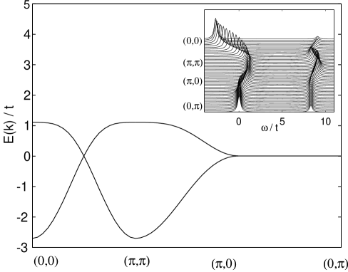
FIG. 1.: Momentum dependence of the lower Hubbard band for $U=8t$, $n=0.79$, and $T=0.01t$. From the spectral function shown in the inset, it clear that the spectral weight in the lower Hubbard band resides entirely on the curve with a flat dispersion near $(\pi,\pi)$. The spectral weight in the upper Hubbard band is also shown.

The two bands in Fig. (1) correspond to $E_{1}({\mathbf{k}})$ and $E_{2}({\mathbf{k}})=E_{1}({\mathbf{k}}+Q)$. As the spectral function attests (see inset Fig. (1)), only one of the bands has a non-zero weight as is expected in the absence of staggered currents. The spectral function shown in the inset $-1/\pi{\rm Im}\sum_{mn}\left(G^{AA}+G^{AB}\right)_{mn}$ in actuality consists of a series of $\delta$-functions. Each peak has been given an artificial width of $0.2t$.

To investigate the stability of staggered currents, we set $p_{1}$ to a fixed value, $p_{\rm in}$, and determine the self-consistent values of all correlation functions upon successive iteration. We then obtained the output value of $p_{1}=p_{\rm out}$ by using Eq. (22). Staggered current vorticity is stable if $p_{\rm in}=p_{\rm out}$ or equivalently, $\lambda(p_{\rm in})=p_{\rm out}/p_{\rm in}=1$ and $d\lambda/dp_{\rm in}<0$. As is evident from Fig. (2), $\lambda<1$ and it is a decreasing function of $p_{\rm in}$, proving that staggered currents are absent for $U=8t$, $V=0.0$ and $T=0.01t$. This can also be seen from the inset of Fig. (2) which contains the average energy per particle ($\langle H\rangle$) as a function of $p_{1}$. The minimum value of the energy corresponds to $p_{1}=0$, further affirming the absence of staggered currents.

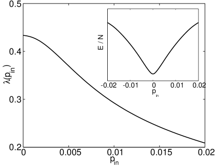
FIG. 2.: Staggered flux stability parameter $\lambda$ vs the input value ($p_{\rm in}$) for the imaginary part of the correlation function, $p$. The flux phase is stable if $\lambda=1$ and $d\lambda/\d{p}_{\rm in}<0$. Because $\lambda<1$, staggered currents are absent. The inset demonstrates that the energy per particle is a minimum when $p$ is real, thereby implying an absence of the staggered current phase. Here $U=8t$ and $V=0$.

Although the flux phase is absent for the parameters above, we can examine the tendency towards such ordering as a function of density for a sufficiently small value of $p_{1}$ such that $\lambda\approx\lambda(0)$, the maximum value of $\lambda$ as shown in Fig. (2). Shown in Fig. (3) is the density dependence of the tendency towards staggered flux ordering for $p_{1}=0.001$ for three values of the on-site Coulomb repulsion, $U=8t,4t,2t$, $V=0.0$ and $T=0.01t$.

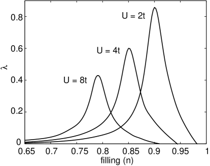
FIG. 3.: Density dependence of the staggered current stability parameter. Half-filling corresponds to $n=1$.

As is evident, stable staggered currents are most likely at small values of $U$ and as the density approaches half-filling as has been reported earlier in mean-field studies of the $t-J$ model[2]. However, for the parameters of the Hubbard model that are relevant for the copper oxides, $U\gg t$, such ordering is absent at this level of theory. Going beyond the static approximation involves including quantum fluctuations. Such processes can only suppress ordering. Hence, we conclude that for $U\gg t$, the Hubbard model (with $V=0$) cannot sustain staggered flux ordering.

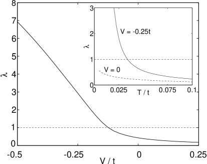
FIG. 4.: Staggered current stability parameter as a function of the nearest-neighbour Coulomb interaction, $V$ for $n=0.79$, $U=8t$ and $T=0.01t$. For $V<0$, the stability parameter exceeds unity leading to an onset of staggered flux order. From the inset, the onset temperature when $V=-0.25t$ is $T=0.33t\approx 160K$.

What about nearest-neighbour Coulomb interactions? As is evident from Fig. (4), the flux phase is destabilised even further for $V>0$. However, for $V<0$, $\lambda$ crosses unity and staggered flux ordering obtains. This is the primary result of this study. The inset shows the temperature dependence of $\lambda$ for $V=0.0$ as well as for $V=-0.25t$. The onset temperature for the flux phase is $T\approx 0.033t\approx 160K$. For $V=0.0$, $\lambda$ is relatively flat indicating further that even at $T=0$, such ordering is absent. To examine the impact of the staggered current on the band structure, we recalculated the lower Hubbard band for $V=-0.25t$, $n=0.79$, $U=8t$ and $T=0.01t$. From Fig. (5), we see that a non-zero staggered current vorticity has opened a gap near the Fermi energy along the $(\pi,0)-(0,\pi)$ direction. The inset shows more clearly that the Fermi level lies in the gap near the $(\pi,0)$ and $(0,\pi)$ regions. The position of the Fermi energy relative to the gap edge is doping dependent.

Our work clearly shows that for the parameters relevant to the copper oxides, staggered current vorticity cannot be stabilized unless attractive interactions are present. Further, the apparent doping dependence (see Fig. (3)) of the staggered current is not entirely consistent with competing order in the underdoped regime. Hence, either staggered flux order is irrelevant to the copper oxides or at least nearest neighbour attractions are essential to their stabilization. An obvious source of such an attraction are local phonon modes as has been discussed recently[8]. Our work suggests (assuming the flux phase is relevant) that the strange phenomenology of the cuprates arises from cooperation between phonons and strong on-site Coulomb repulsions.

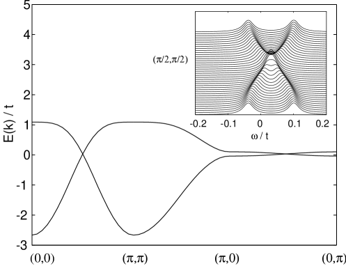
FIG. 5.: Lower Hubbard energy bands and spectral function for $n=0.79$, $V=-0.25t$ and $U=8t$. The presence of a gap along the $(\pi,0)-(0,\pi)$ direction with a node at $(\pi/2,\pi/2)$ is indicative of $d_{x^{2}-y^{2}}$ order.

REFERENCES

[1]S. Chakravarty, R. B. Laughlin, D. K. Morr, and C. Nayak,
cond-mat/0005443.
[2]I. Affleck and J. B. Marston, Phys. Rev. B 37,
3774 (1988); J. B. Marston and I. Affleck, Phys. Rev. B 39, 11538 (1989);
T. C. Hsu, J. B. Marston, and I. Affleck, Phys. Rev. B 43, 2866 (1991);
see also J. B. Marston and A. Sudbo, cond-mat/0103120.
[3]D. A. Ivanov,
P. A. Lee, X.-G. Wen, Phys. Rev. Lett. 84, 3958 (2000).
[4]P. W. Leung, cond-mat/0007068.
[5]D. J. Scalapino, S. R. White, and I. Affleck,
cond-mat/0011098.
[6]T. D. Stanescu, I. Martin, and P. Phillips,
Phys. Rev. B 62, 4300-4308 (2000).
[7]F. Mancini, Phys. Lett. A 249,
231 (1998); for a review see S. Avella, F. Mancini, D. Villani, L. Siurakshina, V. Yu. Yusahnkhai, Int. J. Mod. Phys. B 12, 81 (1998).
[8]A. Lanzara, et. al. cond-mat/0102227; see also
R. S. Markiewicz, cond-mat/0102453.