Free energy and molecular dynamics calculations for the cubic-tetragonal phase transition in zirconia

Abstract

The high-temperature cubic-tetragonal phase transition of pure stoichiometric zirconia is studied by molecular dynamics (MD) simulations and within the framework of the Landau theory of phase transformations. The interatomic forces are calculated using an empirical, self-consistent, orthogonal tight-binding (SC-TB) model, which includes atomic polarizabilities up to the quadrupolar level. A first set of standard MD calculations shows that, on increasing temperature, one particular vibrational frequency softens. The temperature evolution of the free energy surfaces around the phase transition is then studied with a second set of calculations. These combine the thermodynamic integration technique with constrained MD simulations. The results seem to support the thesis of a second-order phase transition but with unusual, very anharmonic behaviour above the transition temperature.

I Introduction

A large class of advanced ceramics are solid solutions of zirconia (ZrO₂) with cubic stabilising oxides like Y₂O₃, MgO or CeO, and are generally called stabilized zirconias. The long list of functional applications includes high-temperature devices, thermal barriers, and oxygen sensors. Moreover, partially stabilized zirconias represent a new generation of structural materials, by far the toughest ceramic oxides, strengthened by the mechanism called transformation toughening. The processing and service conditions of these materials involve phase transformations whose underlying physics is still a subject of controversy. One of these is the high-temperature cubic-tetragonal phase transition which is the subject of the present paper.

Zirconia is monoclinic ($m$) at low temperatures, [1, 2, 3] tetragonal ($t$) between 1400 and 2570 K, [4, 5] and cubic ($c$) up to the melting point of 2980 K. [6, 7] High-temperature X-ray experiments on stabilized zirconia revealed the existence of a $c\leftrightarrow t$ phase transition between 2300 and 2600 K, [8, 9, 10, 11] depending on the atmosphere, but the mechanism of the transformation still has not been fully explained. The $c$ and $t$ unit cells are shown in Figure 1: note the characteristic tetragonal distortion of the oxygen sublattice in the $t$ phase.

It is not possible to quench to low temperature the $c$ and $t$ forms of pure zirconia, hence the experiments are difficult because of the high temperatures involved. Alternatively, the $c$ and $t$ structures may be stabilized at low temperatures by impurities. The available measurements are mostly done on stabilized samples. This simplifies the experimental procedure but complicates the interpretation of the results, because, besides the equilibrium $t$ phase, other metastable tetragonal structures are observed in stabilized crystals, denoted by $t^{\prime}$ and $t^{\prime\prime}$. The former is the microstructure of a solid solution quenched from the field of stability of the $c$ phase into the biphasic $c+t$ one. [12, 13] The $t$ and $t^{\prime}$ forms are the same phase, they belong to the space group $P4_{2}/nmc$, but have different composition; [14] $t^{\prime}$ is also called non transformable because it does not spontaneously transform to the $m$ phase. The $t^{\prime\prime}$ structure is observed in the ZrO₂-ErO_1.5 [14] and ZrO₂-Y₂O₃ [15] systems, and has a cubic unit cell with the oxygen sublattice tetragonally distorted.

The microstructure of samples rapidly cooled from the $c$-phase region presents twinned domains separated by antiphase boundaries. The nature and composition of these domains is related to the phase transition mechanism and has been a subject of controversy. Originally they have been interpreted as the result of a diffusionless martensitic reaction. [16, 17, 18, 19] Later, Heuer and Rühle [20] suggested that the transformation could be $non$-martensitic: homogeneous, massive, and displacive. Similarly, the observations of Lantieri et al. [21] were interpreted to mean that the $c\rightarrow t^{\prime}$ transformation is diffusionless but non martensitic, and that the transformation always goes to completion. The same authors later proposed that the transition could be heterogeneous of the first-order with nucleation. [22] According to Sakuma, [23] the transition is instead second-order.

The temperature evolution of the tetragonality $c/a$ and of the anion sublattice distortion has been followed by Yashima et al. [14] in the ZrO₂-ErO_1.5 system. They showed that both order parameters depend continuously on the temperature and suggested that “the transition has the nature of a higher-order phase transition”.

Several attempts have been made in order to include this transformation in phenomenological theories. Hillert and Sakuma [24] expanded the free energy in terms of the defect concentration and assumed the transition to be second-order. Fan and Chen [25] used the time-dependent Ginzburg-Landau theory to expand the free energy of the transformation, treating it as a first-order one. The transformation was instead assumed to be second-order in the Landau energy expansion of Katamura and Sakuma. [26]

The theoretical treatment of the $c\leftrightarrow t$ transition is simpler in stoichiometric zirconia: this is a case similar to the $c\leftrightarrow t$ phase transition in BaTiO₃, where, according to symmetry considerations, the transformation could be either first or second order. A free energy Landau expansion for zirconia, involving the tetragonality of the cell only, without the distortion of the oxygen sublattice, inevitably predicts a first-order transformation. [27] But the inclusion of the latter in the Landau expansion opens the possibility for a second-order transition. [28] As already pointed out [29] the coupling between the order parameters may change the order of the transition from second to first.

In the case of BaTiO₃ it has been possible to measure the order parameters very close to the transition temperature [30, 31] and to establish the order and the mechanism of the transformation. Analogous experiments are difficult in pure zirconia because of the high transformation temperature. The neutron diffraction analysis of Aldebert and Traverse [6] provides the most complete thermomechanical description of pure $c$ and $t$ zirconia at high temperature. Aldebert and Traverse observe that: (i) The tetragonal distortion of the oxygen sublattice persists in the whole field of stability of the $t$ structure. (ii) The tetragonal distortion of the oxygen ions vanishes in the $c$ structure. (iii) The volume thermal expansion is linear and very close to isotropic up to near the transition point. As a consequence the $c/a$ ratio is almost temperature-independent over a wide range of temperatures, and sharply decreases near the transition temperature. (iv) The isotropic Debye-Waller factors of both species strongly increase before the transition temperature: the authors interpret it as a possible structural phenomenon anticipating the phase transition which could increase the ionic mobility.

The plan of the present paper is as follows. In Sec. II we introduce the main theoretical tools we have used to study the phase transition: the Landau theory of phase transformations, the thermodynamic integration technique, the constrained dynamics and the analysis of the order parameter fluctuations. The results are discussed in Sec. III. The phase transition mechanism was investigated using two sets of calculations. The first one, described in Sec. III A, is a traditional Molecular Dynamics (MD) analysis with which we observed the softening of a particular vibrational frequency. The second one, described in Sec. III B, combines the thermodynamic integration technique with constrained MD simulation to calculate the free energy surfaces around the phase transformation. We summarize the results in the final section.

II Theory

A Landau theory of the phase transition

1 Order parameters

The Landau theory of phase transformations [32] describes the relationship between two crystal structures which share a common symmetry group $G$₀. The disappearance of a particular symmetry operation is quantitatively described by order parameters, which are zero in the high symmetry phase and become non-zero in the low symmetry one.

Our preliminary analysis [29] of the $c\leftrightarrow t$ phase transformation, based on 0 K calculations, showed that the transformation is driven by the distortion of the anion sublattice which is described by the primary order parameter $\delta$. This is a measure of the distance between each oxygen atom and the corresponding centrosymmetric position it occupied in the $c$ structure. The $T=0$ K calculations of certain phonon frequencies of the $c$ phase show that a frequency of vibration at the $X$ point of the BZ is imaginary. [29, 33, 34] This phonon, labelled $X_{2}^{-}$, involves the oxygen sublattice only, and is shown in Figure 1. It transforms according to the $A_{2}$ irreducible representation of the little co-group of the $X$-point $D_{4h}$. The star of $D_{4h}$ contains three equivalent points, consequently the order parameter describing the tetragonal distortion has three components: $\delta_{x}$, $\delta_{y}$, and $\delta_{z}$.

In transforming to the $t$ phase, the primitive unit cell doubles, so that the phonon corresponding to $X_{2}^{-}$ is at the $\Gamma$ point, and is generally labelled $A_{1g}$. Nevertheless, in order to unify the description for both the $c$ and the $t$ structures, we will not use this convention and we will always refer to the soft mode as the $X_{2}^{-}$ one, also in the $t$ phase.

Besides the tetragonal distortion of the oxygen sublattice, it is necessary to capture the change of the unit cell shape. This is done by introducing auxiliary order parameters $\eta_{i}$ defined in terms of the strain tensor $\epsilon$. We decompose the six independent components of the strain tensor into irreducible representation of the $O_{h}$ cubic point group in Table I.

It was shown previously that, at equilibrium, each auxiliary order parameter is second-order in $\delta$. [29, 35] From now on, the order of the expansion terms will be expressed with respect to the order in $\delta$, therefore, as an example, a term like $\delta_{x}^{2}\eta_{1}$ is fourth order.

2 Energy expansion

The Landau theory assumes that the appropriate thermodynamic potential of the crystal $\Phi$ can be expanded in powers of the order parameters about the transition point. The Taylor expansion of $\Phi$ must be invariant under the symmetry operations of the high symmetry phase. As a consequence, the allowed terms in the expansion have to be symmetry-invariants as well, and can be found using group theory. The terms in the energy expansion will be polynomials in the strains $\epsilon_{i}$ and displacements $\delta_{i}$ of Table I. We constructed all the possible polynomials up to the sixth-order and symmetrized them with respect to the symmetry operations of the cubic point group $O_{h}$. The resulting invariants are shown in Table II.

This analysis showed that all the third-order invariants are identically zero, which is a necessary (but not sufficient) condition for a phase transition to be second-order. We already mentioned that the instability appears at the boundary of the BZ, therefore it halves the number of symmetry elements, and this is a further condition allowing the $c\leftrightarrow t$ phase transition to be second-order. [32]

In order to keep the discussion as simple as possible, at this stage we assume the phase transition to be second-order, truncating the Taylor expansion at the fourth-order term in $\delta$. The possible importance of the higher order terms will be discussed later. The energy expansion, expressed in terms of the basis function defined in Table II, is as follows:

$$F = F_{0}+\frac{a_{2}}{2}A_{2}\!\left(\delta^{2}\right)+\sum_{i=1}^{2}\frac{a_{4i}}{4}A_{4i}\!\left(\delta^{4}\right)$$ (2)

$$+\sum_{i=1}^{3}b_{i}B_{i}\!\left(\epsilon,\delta^{2}\right)+\sum_{i=1}^{3}\frac{c_{i}}{2}C_{i}\!\left(\epsilon^{2}\right)+{\cal O}\left(\delta^{6}\right).$$

$F_{0}$ is the energy of the high-symmetry phase and is a function of the hydrostatic strain $\eta_{1}=Tr($$\epsilon$$)$. The choice of the reference volume fixes $F_{0}$ and the expansion coefficients $a_{2},\,\dots,c_{3}$. In the present case, the energy $F$ was expanded about the minimum of the energy-volume curve for the $c$ structure predicted by the SC-TB calculations. [29]

B Free energy calculation

Free energy surfaces may be calculated directly from MD simulations in terms of ensemble averages by using the thermodynamic integration technique. [36, 37] Here we briefly describe how this method was applied to zirconia.

The thermodynamic integration method allows us to calculate free energy differences between a reference state, for which the internal energy $U_{0}$ is known, and another state of the same system, with internal energy $U$. The idea is to relate the two structures with a switching parameter $\gamma$ which is zero in the reference state and non-zero otherwise. The free energy variation in the infinitesimal change $d\gamma$ may be calculated using standard statistical mechanics:

$$dF=\left\langle\frac{\partial U(\gamma)}{\partial\gamma}\right\rangle_{\bar{\gamma}}d\gamma$$ (3)

This is equivalent to the reversible work done for the structural modification described by $d\gamma$, implicitly assumed to be adiabatic. By $\left\langle\cdots\right\rangle$ we indicate the ensemble average, which has to be calculated at a constant value of $\gamma=\bar{\gamma}$. The free energy difference can be obtained by integrating the previous equation. In the general case, $U(\gamma)$ is not known. The common strategy is to perform several constrained MD simulations at different values of $\gamma$ and then integrate Eq.(3) numerically. Many calculations may be necessary in order to integrate Eq.(3) with sufficient precision.

A knowledge of the functional form of the energy would greatly simplify this procedure, reducing the number of calculations and allowing the analytic integration of Eq.(3). The Landau theory in combination with MD simulations can provide such useful information. In order to apply this formalism, it is necessary to define the thermodynamic variables of Eq.(2) from a MD run at finite temperature. Statistical mechanics allows us to calculate the order parameters by averaging the corresponding time-dependent ones over all the available atomic configurations.

The primitive $c$ cell is unstable with respect to 3 modes of vibration whose frequency is degenerate. The instability appears at the $X$, $Y$, and $Z$ points of the primitive BZ and the corresponding eigenmodes distort the anion sublattice along the $x,y$, and $z$ directions. In the following we consider a supercell which is not the primitive one, and those points, originally at the border of the BZ, are folded in at the $\Gamma$ point. The eigenvectors are therefore real.

Let us denote by $\bf u$ the atomic displacements from a perfect site of the high symmetry phase. We expand $\bf u$ in normal coordinates using the notation of Maradudin et al. [38]:

$${\bf u}(\kappa)=\frac{1}{\sqrt{M_{\kappa}}}\sum_{j}{\bf e}(\kappa|j)\,Q(j).$$ (4)

$\kappa$ and $M_{\kappa}$ label the atoms and their mass in the cell, ${\bf e}(\kappa|j)$ is the eigenvector $j$ at the $\Gamma$ point of the BZ, and $Q(j)$ is the corresponding normal coordinate. We will denote by $|\alpha)$, where $\alpha=x,y,z$, the indexes $j$ describing the soft modes.

Given a general atomic configuration at time $t$ (we now include the time in the notation), we define the time-dependent order parameter as the average displacement along $X_{2}^{-}$ of the $r_{\rm O}$ oxygen atoms of the cell:

$$\delta_{\alpha}(t) \equiv \frac{1}{\sqrt{r_{\rm O}}}\sum_{\kappa}{\bf u}(\kappa,t)\cdot{\bf e}(\kappa|\alpha)$$ (5)

$$\equiv \frac{Q(\alpha,t)}{\sqrt{r_{\rm O}M_{\rm O}}}.$$ (6)

The time averages of these quantities, $\bar{\delta}_{\alpha}$, are the experimentally measurable order parameters which we now take as thermodynamic variables.

The factor $\partial U(t)/\partial\delta_{\alpha}$ entering in Eq.(3) can now be calculated at each time step by applying the definition of $\delta$ given in Eq.(5), and by using the chain rule:

$$\frac{\partial U(t)}{\partial\delta_{\alpha}(t)}=\sqrt{r_{\rm O}M_{\rm O}}\,\,\sum_{\kappa}\left(\frac{\partial U(t)}{\partial{\bf u}(\kappa,t)}\right)\cdot\frac{\partial{\bf u}(\kappa,t)}{\partial Q(\alpha,t)}.$$ (7)

Noting that the eigenvectors are orthonormal and that the first term of the sum is the force ${\bf F}$ acting on the atoms we end up with the following expression:

$$\frac{\partial U(t)}{\partial\delta_{\alpha}(t)}=\sqrt{r_{\rm O}}\,\sum_{\kappa}-{\bf F}(\kappa,t)\cdot{\bf e}(\kappa|\alpha)\,.$$ (8)

Therefore the free energy gradient is calculated from the time average of the atomic forces projected along the $X_{2}^{-}$ mode of vibration:

$$\frac{dF}{d\delta_{\alpha}}=\sqrt{r_{\rm O}}\,\left\langle\sum_{\kappa}-{\bf F}(\kappa,t)\cdot{\bf e}(\kappa|\alpha)\right\rangle_{\bar{\delta}_{\alpha}}\,.$$ (9)

Note that the above average has to be taken on an ensemble with a constant value of order parameter $\bar{\delta}_{\alpha}$, i.e. it is necessary to constrain the order parameters during the MD simulations.

C Constraining the order parameters

The dynamics of canonical and microcanonical ensembles with fixed cell shape automatically constrain the auxiliary order parameters. On the contrary, in order to constrain the dynamics of the primary order parameters and then integrate Eq.(9) from the results of the MD simulation, it is necessary to modify the Lagrangian of the system. [36]

The goal is to obtain an equation of motion describing the time evolution of a system with a fixed order parameter $\bar{\delta}$. This is done by extending the Lagrangian of the unconstrained system ${\cal L}^{u}$:

$${\cal L}={\cal L}^{u}-\sum_{\alpha}\lambda_{\alpha}\sigma_{\alpha}.$$ (10)

The superscript $u$ stands for unconstrained, the $\lambda$’s are the Lagrange multipliers to be calculated and the $\sigma$’s are the functions describing the constraints. Three of them are needed, one for each direction $\alpha$ of the tetragonal distortion:

$$\sigma_{\alpha}(t)=\delta_{\alpha}(t)-\bar{\delta}_{\alpha}=0.$$ (11)

The Lagrangian of the constrained system is obtained from equations (10) and (11), and the corresponding equations of motion are:

$$M_{\rm O}\ddot{\bf u}_{\alpha}(\kappa,t)={\bf F}_{\alpha}(\kappa,t)-\frac{\lambda_{\alpha}(t)}{\sqrt{r_{\rm O}}}\,{\bf e}(\kappa|\alpha).$$ (12)

Where ${\bf u}_{\alpha}$ and ${\bf F}_{\alpha}$ are the $\alpha=x,y,z$ components of the displacement and of the force. The orthonormality of the normal modes of vibration decouples the equations along the three crystallographic directions, simplifying the implementation of the method. Moreover, since the tetragonal distortion involves the anion sublattice only, we need apply the above modified equation only to the $r_{\rm O}$ oxygen atoms. In general, the Lagrange multipliers have to be found numerically, but in the present case (decoupled crystallographic directions and linear constraints) an analytical solution does exist.

The expression of the Lagrange multipliers may be found as follow: (i) Advance the atomic positions with a fake unconstrained MD step. (ii) Use these unconstrained coordinates to find the multipliers which exactly satisfy the constraints. (iii) Use these values of $\lambda$’s to perform the true MD step which satisfies the constraining equations by construction. Here we specify this procedure for the leapfrog Verlet algorithm.

Given a set of atomic positions ${\bf u}(t)$ which satisfy the constraining equations (11), the fake step involves solving the equation of motion corresponding to the Lagrangian ${\cal L}^{u}$. By doing so, the set of unconstrained coordinates ${\bf u}^{u}(t+\Delta t)$ is obtained. These are related to the constrained atomic positions ${\bf u}(t+\Delta t)$ as follows:

$${\bf u}_{\alpha}(\kappa,t+\Delta t)={\bf u}_{\alpha}^{u}(\kappa,t+\Delta t)-\frac{\lambda_{\alpha}(t)\,\Delta t^{2}}{\sqrt{r_{\rm O}}\,M_{\rm O}}\,{\bf e}(\kappa|\alpha).$$ (13)

Applying the definition (5) to these coordinates, a similar relationship may be found for the order parameters.

$$\delta_{\alpha}(t+\Delta t)=\delta_{\alpha}^{u}(t+\Delta t)-\frac{\lambda_{\alpha}(t)\,\Delta t^{2}}{r_{\rm O}\,M_{\rm O}}$$ (14)

The analytic solution of the Lagrange multipliers is obtained by imposing the constraining equations $\sigma(t+\Delta t)=0$ and then solving the resulting linear equation in $\lambda$:

$$\lambda_{\alpha}(t)=\frac{r_{\rm O}\,M_{\rm O}}{\Delta t^{2}}\left[\delta_{\alpha}^{u}(t+\Delta t)-\bar{\delta}_{\alpha}\right].$$ (15)

The substitution of (15) in (13) gives the constrained coordinates at $t+\Delta t$ in the NVE ensemble:

$${\bf u}_{\alpha}(\kappa,t+\Delta t) = {\bf u}_{\alpha}^{u}(\kappa,t+\Delta t)$$ (17)

$$-\sqrt{r_{\rm O}}\left[\delta_{\alpha}^{u}(t+\Delta t)-\bar{\delta}_{\alpha}\right]{\bf e}(\kappa|\alpha).$$

It is important to notice that using this method, the expressions for the multipliers are functions of both the integrating scheme and any other additional constraints, such as thermostats. The simple case of the leapfrog Verlet algorithm described here has to be slightly modified in order to include the Nosé-Hoover thermostat. [39, 40, 41] The same procedure may be repeated for the NVT ensemble and the resulting equations of motion are:

$$\ddot{\bf u}_{\alpha}(\kappa,t) = \frac{{\bf F}_{\alpha}(\kappa,t)}{M_{O}}$$ (19)

$$-\sqrt{r_{\rm O}}\left[\frac{\delta_{\alpha}(t+\Delta t)-\bar{\delta}_{\alpha}}{\Delta t^{2}}\left(1+\xi(t)\frac{\Delta t}{2}\right)\right]{\bf e}(\kappa|\alpha),$$

where $\xi$ is the thermostat variable.

D Fluctuations

The fluctuations of the instantaneous order parameter $\delta_{\alpha}(t)$ were used to calculate the frequency of a particular vibration directly from the MD run. The central point of this analysis is the calculation of the fluctuation correlation function spectrum:

$$S_{\alpha}(\nu)=\int e^{-i2\pi\nu t}\left\langle\delta_{\alpha}(t=0)\,\delta_{\alpha}(t)\right\rangle dt.$$ (20)

The above dynamic form factor is known to exhibit two important features, [42] a temperature-dependent resonant peak at $\bar{\nu}$, and an additional central peak at $\nu=0$. The relative magnitude of the two peaks depends on the transformation mechanism and on the temperature. This has been proved for phase transition mechanisms as different as order-disorder and displacive. [43] Therefore, without loss of generality, following Padlewski et al. [43], the power spectrum (20) can be modelled as a superposition of two peaks with the following functional form:

$$S_{\alpha}(\nu)=\frac{2AB}{B^{2}+\nu^{2}}+\frac{CD}{D^{2}+\left(\nu-\bar{\nu}_{\alpha}\right)^{2}},$$ (21)

where $A$, $B$, $C$, $D$ and $\bar{\nu}_{\alpha}$ are parameters to be fitted to the calculations. The analytical form of the time-dependent correlation function $S(t)=\left\langle\delta_{\alpha}(t=0)\,\delta_{\alpha}(t)\right\rangle$ may be found by substituting (21) in (20) and passing into the time domain with an inverse Fourier transform:

$$S_{\alpha}(t)=A\,e^{-B\,t}+C\,e^{-D\,t}\cos(2\pi\bar{\nu}_{\alpha}t).$$ (22)

The time-dependent order parameter is calculated from the MD atomic positions. The time correlation function of $\delta_{\alpha}(t)$ is then obtained using the multiple time-origin method [37] and fitted to Eq.(22). The fitting procedure provides both the time correlation function and its Fourier transform.

III MD Simulations

The polarizable self-consistent Tight-Binding model [29, 35] was used to perform two sets of MD simulations. In the first one, standard MD calculations were used to investigate the temperature dependence of the order parameters and to follow the softening of the $X_{2}^{-}$ mode of vibration up to the transition point. In the second one, we combined the constrained MD simulations and the thermodynamic integration technique to calculate the free energy of the $c\leftrightarrow t$ phase transition, to study the nature of the order parameter fluctuations and to explain the high temperature stability of the $c$ phase.

A Standard MD simulations

1 Softening of a vibrational frequency

The time evolution of a system of 96 particles with periodic boundary conditions has been followed at temperatures between 300 and 2200 K. The lattice parameter of the simulation cell were the correspondent experimental values of Aldebert and Traverse, which, where necessary, have been linearly extrapolated at lower temperatures. During each MD run, the temperature has been constrained with a Nosé-Hoover thermostat, [39, 40, 41] and the equations of motion have been integrated for not less then 5 ps with a typical time step of 5 fs. Near the transition point, the time step has been reduced to 2.5 fs and the total simulation time has been increased to 15 ps.

The cell size was constrained by the relatively high number of MD runs necessary to follow the phase transition. In total, we simulated the time evolution of 96 particles for more than 120 ps. As discussed later, the cell size does not change our qualitative description of the phase transition, and the 324-atom unit cell would have just implied a heavier computational effort, without adding further information to the physical picture provided by the smaller cell.

We started the simulations from the crystallographic positions of the tetragonal phase and equilibrated the system at the temperature of 300 K. This temperature is well inside the field of stability of the $m$ phase, however, during the MD simulations, the system remained in the $t$ phase because of the existence of an energy barrier between the two structures. We calculated the vibrational frequencies of the $t$ structure by diagonalising the dynamical matrix at the origin and at the borders of the Brillouin Zone (BZ) along the (100), (110), and (111) directions. This analysis showed that all the vibrational frequencies are real and that the $t$ phase does not spontaneously distort towards the $m$ structure.

In this set of MD simulations we followed the approach of Padlewski et al. [43] described in Section II D, focusing on the instantaneous order parameters $\delta_{\alpha}(t)$ [see Eq. (5)] which fluctuate about the mean value $\bar{\delta}_{\alpha}$. Figure 2 shows the typical time evolution of the primary order parameters for the MD run at T=700 K. Figure 3 shows the fluctuation autocorrelation function $S(\nu)$ and the corresponding frequency spectrum $S(t)$ for the MD run at 700 K: the arrow points at $\bar{\nu}_{z}$, the frequency which softens. It can be seen that the $x$ and $y$ components, corresponding to the transverse optical frequencies, are degenerate.

On increasing the temperature, the softening of the frequency $\bar{\nu}_{z}$ is evident from the dynamic form factor, where the resonant peak shifts. At the same time, the primary order parameter decreases continuously (Figure 4), as experimentally observed in the similar system ZrO₂-12%ErO_1.5. [14] The calculated temperature dependence of the macroscopic order parameter $\bar{\delta}_{z}$ and of the corresponding vibrational frequency, shown in Figure 5, was then interpreted using the Landau theory. We found that the critical exponent for this phase transition is $\beta$=0.35. According to the same theory, the critical exponent $\beta^{\prime}$ for the auxiliary order parameters ($\eta_{2},\eta_{3}$) describing the tetragonality of the cell is bigger then $\beta$. Therefore the $c/a$ ratio should depend more strongly on the temperature than $\delta$.

As the transition temperature is approached, the decrease of the order parameter and of the corresponding frequency is accompanied by an increase in the order parameter fluctuations, which theoretically diverge at $T_{c}$ for a second order phase transition. As a result, it was not possible to follow the complete softening of the frequency: there is a temperature window about $T_{c}$ where, even though long MD simulations allow one to evaluate the average order parameters, it is not possible to calculate the frequency. In this temperature range, the frequency $\bar{\nu}$ is so low that the corresponding peak in the dynamic form factor $S(\nu)$ merges with the central peak and it is not possible to separate them.

The theoretical transition temperature of $\approx$1800 K is $\approx$30% lower than the experimental value of $\approx$2600. [6] This may be explained by noting that the first-principles calculations underestimate the energy difference between the $c$ and $t$ structures $\Delta U^{t-c}$, which determines $T_{c}$.[29, 44, 45] This is the ab initio energy barrier between the minima of the double well, which was used to parametrize the SC-TB model. In particular the SC-TB results underestimate the experimental $\Delta U^{t-c}$ by 30%, which is consistent with the underestimate of the transition temperature.

According to the renormalized phonon group theory, [46] $\bar{\nu}^{2}$ depends linearly on the temperature in both the regions $T<T_{c}$ and $T>T_{c}$, and the correspondent slopes are related by the following relationship:

$$R=\left(\frac{d\bar{\nu}^{2}}{dT}\right)_{T<T_{c}}/\left(\frac{d\bar{\nu}^{2}}{dT}\right)_{T>T_{c}}=-2.$$ (23)

However, our simulations at $T>T_{c}$ suggest that the $c\leftrightarrow t$ phase transition in zirconia has a different behaviour from the ideal case described by Eq.(23), because no frequency was observed above $T_{c}$.

The exploration of the high temperature region of the zirconia phase diagram has been carried out in two stages. As a first attempt, we continued the MD simulations on the system described above, simply increasing the temperature. This has been done up to 2200 K. The time autocorrelation function (22) of these simulations exponentially decayed without showing any structure. As a result, the central peak dominated the corresponding dynamic form factor, and therefore it was not possible to isolate the resonant peak at $\bar{\nu}$ from the central one. A possible explanation of this may be proposed by noticing that, according to Eq.(23), for $T>T_{c}$ the slope of $(\frac{d\bar{\nu}^{2}}{dT})$ is half that for $T<T_{c}$. This means that the temperature window around $T_{c}$, in which it is not possible to calculate the frequency, extends more in the high temperature field than in the low temperature one. Probably 2200 K is still in the region of disturbance of the transition point.

In order to verify if the frequency does eventually increase in the high temperature region, we studied a similar system with the same properties of that one described above but with a lower transition temperature. The idea is based on the following argument. It is well established that the relative energetics of the two phases is governed by a double well in the potential energy that depends on volume and $c/a$. [47, 48, 49, 50] We studied in detail its dependence, [29] which is also captured by the Landau expansion (2). Both the hydrostatic and tetragonal strains modify the double well in the same way: the smaller the volume (or the $c/a$ ratio), the smaller the energy difference and therefore the smaller the transition temperature. Incidentally, this is connected to the ab initio underestimate of the energy barrier, which is calculated with the structural parameters corresponding to 0 K.

By exploiting this property of the energy surfaces, we made a new set of MD simulations aimed to explore the temperature range $T>T_{c}$. In these calculations the volume was chosen to lower the transition temperature to $\approx$1300 K and the cell was kept cubic ($c/a=1$) even in the low temperature region. As expected, for $T<T_{c}$, the linear softening of $\bar{\nu}^{2}$ (Figure 5 set b) was obtained for this system as well. The slope was slightly different because in the previous simulations the thermal expansion of the cell was included in the description, while in this case the volume was fixed to the initial value. Because of this we could calculate the frequency up to within $\approx$200 K of the transition temperature. The temperature was then increased to 2000 K. Surprisingly, even in this case, there was no structure in the autocorrelation function $S(t)$ and the expected hardening of the frequency was not observed. This suggests that in the $c$ phase the motion of the oxygen sublattice along the $X_{2}^{-}$ mode of vibration is, in terms of $S(t)$, uncorrelated. This behaviour will be clarified by the free energy surfaces described in Section III B.

B MD simulations at constant $\delta$

In our previous papers [29, 35] we restricted the analysis of the 0 K energy surface to one tetragonal invariant only. By doing so, we defined a simplified version of the energy expansion (2) involving the strain and one component of the primary order parameter. We then fitted the correspondent coefficients, $a_{2}$, $a_{41}$, $b_{1}$, $b_{2}$, $c_{1}$, and $c_{2}$, to the results of total energy calculations. We also showed how the coupling between the primary and auxiliary order parameters could create a critical point where the transformation becomes first order. Here that analysis is extended by exploring the topology of the energy surface in the whole $\delta$ domain, and by following its temperature evolution through the phase transition into the field of stability of the $c$ phase. This sheds light on the mechanism of the phase transformation and on the high-temperature stability of the $c$ phase.

The following results were obtained using a 12-atom unit cell with different $c/a$ ratios (1, 1.01, 1.02) at the 0 K theoretical equilibrium volume of the $c$ structure. Preliminary unconstrained MD simulations were done to explore the effect of the cell size on the physical picture of the phase transformation described in the previous Section. Even in this small system, the frequency $\bar{\nu}_{z}^{2}$ depends linearly on the temperature and the predicted transition temperature is of $\approx 1600$ K. The effect of using a small cell is to shift $T_{c}$ to higher temperatures. This is consistent with the physical picture proposed in Section III A: the autocorrelation function $S(t)$ measures the degree of correlation between the motion of the oxygen atoms along the $X_{2}^{-}$ mode of vibration. We described how the temperature acts on $S(t)$ by reducing the correlation until this is completely lost above $T_{c}$, where the corresponding frequency is soft, and where the structure is $c$. The small cell size and the periodic boundary conditions force the motion of atoms in adjacent cells to be correlated, and therefore counteract the effect of the temperature on $S(t)$. As a result, in the small system, higher temperatures are needed to observe the complete softening of the frequency $\bar{\nu}_{z}$.

The 12-atom and 96-atom supercells have the same temperature dependence of $\delta_{z}$ and $\bar{\nu}_{z}$ but the corresponding curves are shifted to different temperatures. We can therefore conclude that the phase transformation mechanism is the same in the two systems. We shall calculate the free energy of the transition from the MD simulations of the small cell, and assume that the resulting qualitative physical picture applies to bigger cell sizes.

Before exploring the free energy temperature dependence, it is useful to simplify the complete energy expansion (2) by neglecting the order parameters which are unlikely to play an important role in the phase transition. The transformation between the $c$ and $t$ structures does not distort the cell shape as described by the order parameters ($\eta_{4},\eta_{5},\eta_{6}$). It is therefore reasonable to neglect them in the discussion of the following results. Moreover, even though the transformation between the $c$ and the $t$ structure does involve a change in the volume, the energetic contribution of the associated order parameter $\eta_{1}$ is well understood and has already been discussed. Apart from the 0 K case, we will not consider the terms $B_{3}$ and $C_{3}$ in the energy expansion. However, their possible influence on the character of the phase transition in terms of softening of the corresponding elastic constant, will be discussed a posteriori in the final Section III B 3.

1 Topology of the 0 K surface

We start our analysis with the primary order parameter. Two sets of calculations on a stress-free cubic unit cell were used to fit the coefficients $a_{2}$, $a_{41}$, and $a_{42}$. These have been determined by distorting the oxygen sublattice along $\langle\delta 00\rangle$ and along $\langle\delta\delta 0\rangle$. We plot the resulting energy surface, which we take as starting point of our analysis, as a function of two tetragonal invariants in Figure 6. In this simple case, because of the cubic cell, the three components of the primary order parameter are equivalent.

The same set of calculations was then done on a tetragonal cell ($c/a=1.01$), by which we determined the parameters $b_{2}$ and $c_{2}$. The latter is proportional to the elastic constant $C^{\prime}$. The transferability of the parameters was then checked by redoing the calculations for a different tetragonal cell ($c/a=1.02$): Figure 8 shows that the same set of coefficients fit the results for this cell as well. If $z$ is the tetragonal axis, the tetragonality of the unit cell shortens the average interatomic distances in the transverse $x,y$ plane and lengthens them along the tetragonal axis. As a consequence, the energy surface section in the transverse plane $\delta_{x},\delta_{y}$, shown in Figure 7 (a), is similar to the reference one of Figure 6 but shallower and tighter, while it is deeper and broader along $\delta_{z}$ [Figure 7 (b)].

Finally, the same procedure described above was used to fit the remaining coefficients $b_{1}$ and $c_{1}$ by distorting the cell with respect to the order parameter $\eta_{1}$ defined in Table I.

In conclusion, the static calculations show that the 0 K energy surfaces can be captured by Taylor expansion up to fourth-order and are therefore completely defined by the set of coefficients given in Table III.

2 Free energy surfaces

The MD simulations were carried out in the temperature range from 50 K to 2000 K, constraining the primary and secondary order parameters. Let us first focus on the results for the cubic cell, commenting later on the effect of the $c/a$ ratio. The explorations along the directions $\langle\delta 00\rangle$ and $\langle\delta\delta 0\rangle$ fully determine the free energy surfaces to fourth order, therefore we constrained the order parameters along these directions from 0 to 0.7 a.u., using the dynamics described in Section II C. The quantity defined in Eq.(8) was accumulated during the MD run and its time average provided the ensemble average required in Eq.(9). The analytical form (2) of the energy surface was then differentiated along the corresponding direction and fitted to the results of the simulations. For this particular case, the fit provided both the free energy gradient and the free energy itself. This is because we chose the reference energy as the top of the double well for a cubic crystal. The integration of Eq.(9) provides the energy difference $\Delta F$:

$$\Delta F=F(\epsilon,\bar{\delta})-F(\epsilon,\bar{\delta}=0)=\int_{0}^{\bar{\delta}}\left\langle\frac{\partial U}{\partial\delta}\right\rangle_{\bar{\delta}}d\delta.$$ (24)

We arbitrarily set to zero the integration constant for the cubic cell $F(\epsilon=0,\bar{\delta}=0)$. If the cell is tetragonal the same constant is $c_{2}\,C_{2}(\epsilon^{2})/2$. Therefore, the fit of the free energy gradient to the MD simulations of the cubic cell provided the coefficients $a_{2}$, $a_{41}$, $a_{42}$ and $b_{2}$ at the corresponding temperature.

The fit to the computed results along the $\langle\delta 00\rangle$ and the corresponding free energy profiles obtained from Eq.(24) are shown in Figures 9 and 10 respectively. The corresponding expansion coefficients are included in Table III. Also at high temperature the fourth order energy expansion well describes the calculated free energy gradients. The temperature acts on the double well by gradually reducing the energy difference between the distorted and undistorted structure. As expected, the energy surface is very flat near the critical temperature, but, surprisingly, it remains quite flat even at higher temperatures, well inside the field of stability of the cubic phase. The energy surfaces above the transition temperature are highly anharmonic.

The unconstrained MD simulations described in the previous Section generated the temperature dependence of the $X_{2}^{-}$ vibration frequency (Figure 5) up to the transition point only. Above the critical temperature it was impossible to calculate the frequency $\bar{\nu}_{z}$, the dynamic form factor $S(\nu)$ being dominated by a wide central peak. The soft frequency $\bar{\nu}_{z}$, together with the large fluctuations of the order parameters $\delta_{z}$, suggests a disordered dynamics of the oxygen sublattice along the $X_{2}^{-}$ mode of vibration. The anharmonicity of the energy surfaces explains this behaviour. It may also explain the fact that the optical-phonon branches are not experimentally observed [51] in cubic stabilized zirconia.

As in other perfect fluorite structures, [52] the vibrational motion of the anions in $c$ zirconia appears to be anharmonic. This is consistent with the neutron powder diffraction experiments of Kisi and Yuxiang [53] on cubic stabilized zirconia (ZrO₂-9.4%Y₂O₃). They measured the temperature dependence of the Debye-Waller factor and proposed different models to fit the data. Both a simple Debye model and a Debye model plus a static disorder component provided a poor fit of the data. A radical improvement of the fit was obtained when an isotropic anharmonic vibration of both species was included in the description.

We may further investigate the nature of the double well temperature dependence by splitting the free energy into its energetic and entropic contributions. The time average of the internal energy $U$ from each constrained MD simulations is plotted in Figure 11. It is clear that the double well in the internal energy is present even at $T>T_{c}$. The internal energy double well is relatively insensitive to the temperature and the 0 K coefficients of Table III provide an excellent fit of the finite temperature results for both the low and high temperature structures. From the definition of $F$, the difference between the free energy calculated with Eq.(24) and the internal energy gives the entropic contribution $TS$ plotted in Figure 12. The high temperature stability of the $c$ phase is therefore ensured by this entropic term which change the shape of the energy surface from double to single welled.

3 Coupling to the elastic strains

The fit of the Landau energy expansion (2) to the calculation results has allowed us to follow the temperature evolution of the free energy surface through the phase transition. The fitting coefficients for each temperature are included in Table III. We can see that at the critical temperature of $\approx 1600$ K, when $a_{2}$ goes to zero, the fourth order coefficient $a_{4}$ is positive. Therefore, in this cell, the phase transition is diffusionless displacive and second order.

If the thermodynamic potential $F$ is expanded in terms of elastic strains as well as $\delta$, the coupling between the primary order parameter and the strain in (2) renormalizes the fourth-order coefficient [32, 54, 55] and could make it small or negative near the transition point. As a result, the transformation may become first-order. This could happen if the temperature reduces an elastic constant $c_{i}$.

In order to see this, let us consider a tetragonal cell at the reference volume, whose tetragonal axis is $z$ and where the oxygen sublattice is distorted along the order parameter direction $\langle 00\delta_{z}\rangle$. With these restrictions the energy expansion (2) has a simplified form:

$$F=F_{0}+\frac{a_{2}}{2}\delta_{z}^{2}+\frac{a_{41}}{4}\delta_{z}^{4}+b_{2}\,\,2\delta_{z}^{2}\,\,\eta_{2}+\frac{c_{2}}{2}\,\,\eta_{2}^{2}+{\cal O}\left(\delta_{L}^{6}\right)\,.$$ (25)

At equilibrium the two order parameters $\delta_{z}$ and $\eta_{2}$ are not independent and the relationship between the two may be found by imposing the equilibrium condition:

$$\frac{\partial F}{\partial\eta_{2}}=0\hskip 14.22636pt\Rightarrow\hskip 14.22636pt\eta_{2}=-\frac{2b_{2}}{c_{2}}\delta_{z}^{2}.$$ (26)

A similar procedure may be repeated for the hydrostatic strain $\epsilon_{xx}+\epsilon_{yy}+\epsilon_{zz}=\eta_{1}$ and the substitution of Eq.(26) back in Eq.(25), together with the corresponding one for $\eta_{1}$, clarifies the combined effect of the coefficients $b_{i}$ and $c_{i}$ on the renormalization of the fourth order coefficient:

$$F=F_{0}+\frac{a_{2}}{2}\delta_{z}^{2}+\left(\frac{a_{41}}{4}-\frac{2b_{2}^{2}}{c_{2}}-\frac{b_{1}^{2}}{2c_{1}}\right)\delta_{z}^{4}+{\cal O}\left(\delta_{z}^{6}\right)\,.$$ (27)

It may be verified that the above formulation is independent of the initial choice of the tetragonal axis.

The coefficients $c_{1}$ and $c_{2}$ are proportional to the bulk modulus and to the elastic constant $C^{\prime}$, respectively. If one or both of these quantities significantly decrease with temperature, the correspondent term in Eq.(27) may dominate the sign of the fourth-order coefficient, making it very small or negative. At 0 K the coupling terms $2b_{2}^{2}/c_{2}$ and $b_{1}^{2}/2c_{1}$ reduce the fourth-order coefficient by $16$% and $4$% respectively. Because of this difference we focused our attention on the elastic constant $C^{\prime}$. Experimentally, the high temperature data [51, 56, 57] do not show any anomalous temperature dependence of the elastic constants, with a general decrease of $\approx 15-20$% between 300 and 1700 K. If this is valid for pure zirconia as well, we may anticipate that the degree of softening of the elastic constants will not affect the character of the phase transition.

The calculations described above for the cubic cell have been repeated for two tetragonal cells with $c/a=1.01$ and $1.02$. The constrained MD simulations along the $\langle\delta 00\rangle$ direction allowed the fit of the coupling coefficient $b_{2}$ to each temperature. Therefore it has been possible to obtain the temperature and $c/a$ dependent free energy curve along this direction. However, in this case we are interested in the relative position of the free energy surfaces for the different cells, depending on the integration constant $F(\epsilon,\delta=0)=c_{2}\,C_{2}(\epsilon^{2})/2$. In principle one could calculate $c_{2}$ by a simple thermodynamic integration, but this would require monitoring the stress, which is not yet implemented in the current program. Therefore we decided to continue the analysis by choosing an extreme scenario, which would be a strong temperature dependence of $C^{\prime}$. With a large safety margin with respect to the experimental values, we linearly reduced this elastic constant by $75$ % from 200 to 50 MPa between 0 and 2000 K.

With this assumption, the sections of the free energy surfaces at different temperatures between 500 and 2000 K are plotted in Figure 13 as a function of $\delta$ and $c/a$. As experimentally observed, [6] the tetragonal cell with $c/a=1.02$ is thermodynamically stable up to very near $T_{c}$ where the minimum configuration goes from $(c/a=1.02,\delta=0.4)$ to $(c/a=1,\delta=0)$ quickly but continuously. We believe that the sudden change of the order parameters, due to the flat energy surfaces near the transition point and therefore to the anharmonicity of the material, may explain the fact that this phase transition has been considered to be first order in the early studies.

It is interesting to note that both the $a_{41}$ and the coupling coefficient $b_{2}$ decrease with temperature (Table III). Because of this, even with the large postulated softening of $C^{\prime}$, the renormalization of the fourth-order coefficient in Eq.(27) does not increase with temperature. From the data of Table III, we find that at $T_{c}$, the term $2b_{2}^{2}/c_{2}$ is still only $10$% of $a_{41}/4$, less than in the 0 K case. These results show that even a large softening of the elastic constant $C^{\prime}$ does not change the character of the phase transition, which remains displacive second order.

Figure 13 shows also that, above the transition temperature, the minimum energy corresponds to the cubic cell and therefore the results about the high temperature structural stability of the $c$ phase discussed in the previous Section remain valid.

IV Conclusions

The $c\leftrightarrow t$ phase transition of pure stoichiometric zirconia has been studied from different theoretical perspectives. Both symmetry arguments and the lattice dynamical analysis suggested that this transformation might be second-order. In the 0 K perfect $t$ structure, the primary order parameter $\delta$ has a clear definition in terms of the displacement of the oxygen atoms away from their centrosymmetric position, which define a zone boundary phonon $X_{2}^{-}$. But the same definition cannot be directly applied to a finite temperature atomic configuration. Instead, we defined the more general macroscopic thermodynamic variable as an ensemble average of the displacements of the O atoms projected onto the $X_{2}^{-}$ zone boundary phonon coordinate. The corresponding frequency of vibration was then calculated directly from the MD simulations by applying standard statistical mechanics techniques.

The temperature evolution of both the equilibrium order parameter $\delta$ and of the corresponding frequency $\nu$ was then followed during the MD run. The results of these simulations have been interpreted with the Landau theory: the critical exponent of 0.35 fitted to the results is between the extreme values of 0.5 and 0.25 corresponding to a second-order and to a tricritical phase transition.

Approaching $T_{c}$ from the field of stability of the $t$ phase, the order parameter $\delta$ gradually decreases up to very near the transition point, as in a displacive second-order phase transformation. In a temperature window about $T_{c}$, the large fluctuations of the order parameter degrade the quality of the averages achievable from MD simulations, but we were able to observe $\nu^{2}$ decreasing linearly with $T$ by some 70 %. In contrast to the prediction of the Landau theory, no increase of that frequency in the field of stability of the $c$ phase was observed. At high temperatures the dynamics of the oxygen sublattice revealed a high degree of mobility of the anions and a low correlation between their motion along the $X_{2}^{-}$ vibrational mode.

In order to clarify these observations, we calculated the free energy surfaces relating the two structures at different temperatures, combining constrained MD simulations and the thermodynamic integration technique. These calculations showed that the high temperature stability of the $c$ structure is due to the entropic contribution $T\Delta S$ and not to a variation of the internal energy profile. Moreover, we showed that the energy surfaces of the $c$ phase are highly anharmonic, not only at the transition temperature, but also well above $T_{c}$. This confirms and may explain in terms of thermodynamic quantities the absence of the optical modes of vibration in the experimental spectra of Liu et al., [51] and the postulated uncorrelated “fluidlike” motion of the oxygens about their centrosymmetric position. Similarly, the experimentally observed increase of the ionic conductivity and the “structural phenomenon” mentioned by Aldebert and Traverse [6] may possibly be connected with the soft dynamics of the oxygen sublattice caused by the flat energy surfaces.

Our analysis revealed the peculiar character of the $c\leftrightarrow t$ transformation in zirconia. Approaching $T_{c}$ from below, the variation of the free energy surfaces seems to support the thesis of a $t\rightarrow c$ displacive second-order phase transition. On the contrary, approaching $T_{c}$ from above, it is not possible to follow the softening of a particular phonon mode. The entropic term $T\Delta S$ eliminates the double well in the free energy, and frees the atoms to move along that mode without an energy cost and without a well defined vibrational frequency. This is more akin to the high temperature phase in an order-disorder phase transformation.

TABLE I.: Order parameters for the $c\leftrightarrow t$ phase transition decomposed into irreducible representations of the $O_{h}$ cubic group.

order parameters	irrep
$\left(\delta_{x},\delta_{y},\delta_{z}\right)$		$T_{1}$
$\,\,\,\eta_{1}$	$\left(\epsilon_{xx}+\epsilon_{yy}+\epsilon_{zz}\right)$	$A_{1}$
$(\eta_{2},\eta_{3})$	$\left[\left(2\epsilon_{zz}-\epsilon_{xx}-\epsilon_{yy}\right),\sqrt{3}\left(\epsilon_{xx}-\epsilon_{yy}\right)\right]$	$E$
$(\eta_{4},\eta_{5},\eta_{6})$	$\left(\epsilon_{xy},\epsilon_{yz},\epsilon_{zx}\right)$	$T_{2}$

TABLE II.: Polynomials in the order parameters of Table I which are invariants under the set of transformations belonging to $O_{h}$.

$A_{2}(\delta^{2})$	$(\delta^{2}_{x}+\delta^{2}_{y}+\delta^{2}_{z})$
$A_{41}(\delta^{4})$	$(\delta^{4}_{x}+\delta^{4}_{y}+\delta^{4}_{z})$
$A_{42}(\delta^{4})$	$(\delta^{2}_{x}\delta^{2}_{y}+\delta^{2}_{y}\delta^{2}_{z}+\delta^{2}_{z}\delta^{2}_{x})$
$B_{1}(\epsilon,\delta^{2})$	$(\delta^{2}_{x}+\delta^{2}_{y}+\delta^{2}_{z})(\epsilon_{xx}+\epsilon_{yy}+\epsilon_{zz})$
$B_{2}(\epsilon,\delta^{2})$	$(2\delta^{2}_{z}-\delta^{2}_{x}-\delta^{2}_{y})(2\epsilon_{zz}-\epsilon_{xx}-\epsilon_{yy})$
	$\,+3(\delta^{2}_{x}-\delta^{2}_{y})(\epsilon_{xx}-\epsilon_{yy})$
$B_{3}(\epsilon,\delta^{2})$	$(\delta_{x}\delta_{y}+\delta_{y}\delta_{z}+\delta_{z}\delta_{x})(\epsilon_{xy}+\epsilon_{yz}+\epsilon_{zx})$
$C_{1}(\epsilon^{2})$	$(\epsilon_{xx}+\epsilon_{yy}+\epsilon_{zz})^{2}$
$C_{2}(\epsilon^{2})$	$(2\epsilon_{zz}-\epsilon_{xx}-\epsilon_{yy})^{2}+3(\epsilon_{xx}-\epsilon_{yy})^{2}$
$C_{3}(\epsilon^{2})$	$(\epsilon^{2}_{xy}+\epsilon^{2}_{yz}+\epsilon^{2}_{zx})$

TABLE III.: Coefficients for the Landau energy expansion (2) at the 0 K equilibrium volume of the $c$ cell: $a_{2}$ and $a_{42}$ in Ry/$a_{0}^{2}$, $a_{41}$ in Ry/$a_{0}^{4}$, and $c_{2}$ in Ry, where $a_{0}$ is the Bohr radius. The coefficients $b_{1}=-0.363$ Ry/$a_{0}$ and $c_{1}=16.768$ Ry complete the 0 K set. See text for the temperature dependence of $c_{2}$.

T (K)	$a_{2}$	$a_{41}$	$a_{42}$	$b_{2}$	$c_{2}$
0	-0.0534	0.347	1.825	-0.0763	1.228
50	-0.0478	0.330	1.191	-0.0749	1.204
500	-0.0258	0.235	0.873	-0.0705	0.998
1000	-0.0143	0.191	0.751	-0.0384	0.768
1500	-0.0058	0.184	0.661	-0.0354	0.537
2000	0.0030	0.152	0.273	—	0.307

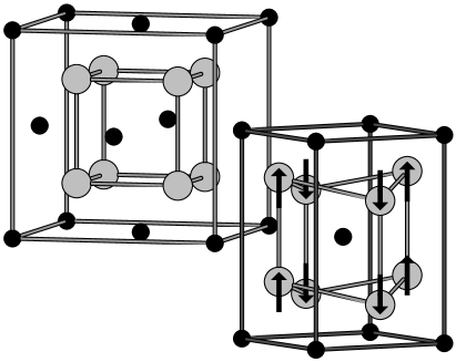
FIG. 1.: Cubic and tetragonal structures of ZrO₂. Light and dark circles denote oxygen and zirconium atoms respectively. Arrows represent the structural instability of the oxygen sublattice along the $X_{2}^{-}$ mode of vibration.

FIG. 2.: Time-dependent order parameters at 700 K: $\delta_{x}$ and $\delta_{y}$ oscillate around 0, $\delta_{z}$ around $\bar{\delta}_{z}$, the value of the macroscopic order parameter.

FIG. 3.: Time correlation functions (top) and corresponding Fourier transforms (bottom) of the time-dependent order parameters $\delta_{x}$, $\delta_{y}$, and $\delta_{z}$.

FIG. 4.: Temperature dependence of the macroscopic order parameter $\bar{\delta}_{z}$. The symbols ($\bullet$) are the results of the calculations. The continuous solid eye-line is extrapolated in the region near $T_{c}$ where the large fluctuations in $\delta_{z}$ make the averaging procedure inaccurate.

FIG. 5.: Calculation results of the frequency squared $\bar{\nu}_{z}^{2}$ vs. temperature for two simulation sets : (a) tetragonal cell with temperature-dependent lattice parameters taken from experiment, [6] (b) Cubic cell with temperature-independent lattice parameter (see text).

FIG. 6.: Section of the 0 K energy surface for the cubic cell. The isoenergetic contours are plotted on the base every 0.3 mRy/ZrO₂.

FIG. 7.: 0 K energy surfaces for a tetragonal cell with the tetragonal axis along $z$: (a) section in the $\delta_{y},\delta_{x}$ plane, (b) section in the $\delta_{z},\delta_{x}$ plane. The isoenergetic contours are plotted on the base every 0.3 mRy/ZrO₂.

FIG. 8.: Transferability of the 0 K energy-expansion coefficients between different tetragonal cells with the tetragonal axis along $z$. Projections of the corresponding energy surfaces along the high-symmetry order-parameter directions $\langle 00\delta\rangle$ (a), and $\langle\delta\delta 0\rangle$ (b).

FIG. 9.: Temperature-dependent free energy gradients calculated using Eq.(9) and corresponding fit via the analytic form derived from the Landau theory (2). Projection along the order parameter direction $\langle 00\delta\rangle$.

FIG. 10.: Temperature evolution of the free energy profiles projected along the order parameter direction $\langle 00\delta\rangle$. The symbols ($\bullet$) are the 0 K calculations, the thick solid lines are the result of the thermodynamic integration and correspond to the temperatures 50, 500, 1000, 1500, and 2000 K.

FIG. 11.: Double well in the internal energy along the order parameter direction $\langle 00\delta\rangle$: the solid line correspond to the 0 K calculation, the symbols are the averaged internal energies from the constrained MD simulation.

FIG. 12.: Entropic contribution to the phase transition obtained by applying the definition of the Helmholtz free energy $\Delta F=\Delta U-T\Delta S$ to the data shown in Figures 10 and 11.

FIG. 13.: Free energy profiles projected along the order parameter direction $\langle 00\delta\rangle$ for cubic and tetragonal cells below and above the transition temperature.