A Microscopic Model for Packet Transport in the Internet

Abstract

A microscopic description of packet transport in the Internet by using a simple cellular automaton model is presented. A generalised exclusion process is introduced which allows to study travel times of the particles (’data packets’) along a fixed path in the network. Computer simulations reveal the appearance of a free flow and a jammed phase separated by a (critical) transition regime. The power spectra are compared to empirical data for the RTT (Round Trip Time) obtained from measurements in the Internet. We find that the model is able to reproduce the characteristic statistical behaviour in agreement with the empirical data for both phases (free flow and congested). The phases are therefore jamming properties and not related to the structure of the network. Moreover the model shows, as observed in reality, critical behaviour ($1/f$-noise) for paths with critical load.

, , , , and

1 Introduction

In recent years the Internet has become the most popular medium for information transfer in the world. Terms like ‘e-mail’ and ‘e-commerce’ are nowadays well known to almost everybody. Due to the enormous increase of Internet users and a still growing demand the network already reaches its maximum capacity at some times. Almost every user has been annoyed by decreasing transfer rates and increasing waiting times caused by congestions in the Internet. The heterogeneity of the network, e.g., due to different transport protocols and operating systems, and its enormous expansion in the last years make it necessary to understand the basic properties of data transport in the Internet for planning new connections and optimising the usage of the existing resources. Especially the influence of routers (network nodes) with low transfer rates, which are considered to be the reason for the congestions, and the collective behaviour of routers are main targets of recent investigations. Real data measurements like those for the ping statistics [1, 2, 3, 4] or the load of a single router [5, 6] on various kinds of networks and their analysis are the basis for a better understanding of Internet traffic. Moreover there are investigations by Huberman and Lukose [7] on the social aspects of the Internet and the “human factor” in the system. Empirical results for the load of single routers show a self-similar behaviour of Internet traffic which Willinger et al. [6] explained as a superposition of ON/OFF sources with heavy tailed distributions of the duration lengths of the ON/OFF-periods. Another method to characterise a nonequilibrium system like an Internet connection is the survey of ping time series, first presented by Csabai [1] and later by Takayasu et al. [2, 8]. Here the travel times of data packets from a source to a destination host and back to the source host, the so-called Round Trip Times (RTT), are measured. The analysis of the respective power spectra shows characteristic statistics for different “traffic” states. One can distinguish a free flow and a jammed phase separated by a transition regime. On the basis of these measurements various models were introduced to reproduce the characteristic stochastic properties. Takayasu et al. [3] proposed a simple model based on the contact process [9] to explain $1/f$-noise in the travel times of data packets and to reproduce the distribution of the congestion duration length of routers. The model of Yuan et al. [10] is based on a reinterpretation of the well-known cellular automaton approach for vehicular traffic [11, 12]. Data transport is realised by changing headways between “moving routers”. This method does not give any access to the travel times of data packets. In [13] a two-dimensional model has been suggested. Measurements of the travel times indicate the existence of a phase transition into a jammed phase. The influence of the structure of the network, namely the branching number, has been investigated in [14] for a simple stochastic model on a Cayley tree.

2 Model

In the Internet traffic data files are divided into small data packets of a definite size. These data packets move, for fixed source and destination hosts, due to the structure of the Internet transportation protocol (TCP/IP), along a temporally fixed route. Therefore the transport between two specific hosts can be viewed as a one-dimensional process. Here we want to investigate the question which properties of Internet traffic can already be understood by considering just the one-dimensionality of these routes, i.e., as jamming properties of the routers. A well known cellular automaton model to describe one-dimensional transportation systems from different fields like the kinetics of biopolymerisation and vehicular traffic is the Asymmetric Simple Exclusion Process (ASEP) [12, 15]. Because of its simple structure it is a well studied nonequilibrium system. An important property of the ASEP is the occurrence of boundary-induced phase transitions [16]. Depending on the inflow and outflow the system can be in different phases separated by (bulk) phase transitions. In order to reproduce the statistical characteristics of Internet traffic we introduce a simple microscopic cellular automaton model with open boundary conditions based on the ASEP by allowing a finite number $B_{n}$ of particles (data packets) on each site (router) $n$. Hereby we take into account that each router has a buffer of finite capacity so that more than one data packet can be stored (multi-allocation of sites). The data packets move with a router specific probability $p_{n}$ to the the next router. This probability determines the amount of traffic at the network node (the current) as well as the statistical behaviour of processing times. The dynamics of the system do not only depend on the probability a data packet moves to the next router, but also on the restriction of the buffers so that a data packet only moves to the next router as far as there is enough space left.
The model is defined on a linear array of $N$ sites (Fig. 1). Each site $n=1,\ldots,N$ represents a router with a buffer which stores $Z_{n}(t)$ particles at time $t$. Each router has a finite capacity $B_{n}$, i.e., $Z_{n}(t)\leq B_{n}$. A particle $i$, representing a data packet, moves with probability $p_{n}$ from site $n$ to the next site $n+1$ as long as the buffer ${n+1}$ is not completely occupied. $p_{n}$ is a time-independent characteristic property of the router $n$, i.e., it does not depend on the load of the buffer itself. The update is performed in parallel for all buffers and the travel times $T_{i}$ of all packets in the system are increased by the discrete time $\Delta t$. The data packets arriving at the last site $N$ are removed with probability $p_{N}$ and their travel times $T_{i}$, i.e., the times needed to travel through the system, are stored.

Figure 1: System consisting of $N=7$ routers with buffer size $B=8$.

At $t=0$ we start with empty buffers at all routers, i.e., $Z_{n}(t=0)=0$. In each time step the following update steps are applied in parallel:

1. As long as the first router $n=1$ is not completely occupied $j_{\text{in}}$ data packets are inserted: $Z_{1}(t+1)=\min(Z_{1}(t)+j_{\text{in}},B_{1})$. The travel times of these packets are set to zero: $T_{i}=0$.

2. The travel times $T_{i}$ of those data packets $i$ present in the system are increased by $\Delta t=1$.

3. At each router $n=1,\ldots,N-1$ the data packets are picked up sequentially in the order of their arrival in the buffer and move with probability $p_{n}$ to the next router $n+1$ as long as this router is not completely occupied ($Z_{n+1}(t)<B_{n+1}$).

4. Data packets in the last router which have not already been moved in the same time step are removed with probability $p_{N}$ and their travel times $T_{i}$ are stored.

Note that data packets in a buffer are stored in a waiting queue and therefore the packets with the highest waiting times in the buffer (not to be confused with the travel time) try to move first. Moreover it is to mention that, due to the stochastic character of the movement and the multi occupation of sites, particles can overtake each other which can not be found in the ASEP. Because of the parallel update each data packet can move only once during each time step. In contrast to [14] no data packets are lost. If $B_{n}=1$ for all $n$ the model is identical to the ASEP (with disorder in the hopping rates) with boundary probabilities $\alpha=1$ and $\beta=p_{N}$.

3 Simulations

First we investigate the phenomenological behaviour of the model. A typical sequence of travel times is shown in Fig. 2. Here the travel times of the data packets are plotted as function of the system time, i.e., the time at which the packet arrives at the end of the system.

Figure 2: Typical sequence of travel times in a system of $N=5$ routers with buffer size $B=128$, $p=0.2$, and $j_{in}=1$.

For the following investigations all routers have an identical buffer size $B=128$. Note that with regard to reality we restrict the number of routers to $N=15$ and the probabilities $p_{n}$ are chosen in such a way to obtain a good agreement with empirical data.

As in the ASEP [15] the state of the system is determined by the smallest of three currents, namely the maximal possible inflow, bulk flow and outflow. The mean maximal flow $j^{\text{max}}_{n}$ through a single router $n$ is given by

$$j^{\text{max}}_{n}=Bp_{n}.$$ (1)

For $j^{\text{in}}_{\text{n}}<j^{\text{max}}_{n}$ the dynamics of the system is governed by the dynamics of the collective behaviour of the routers. In reality congestions occur, when the amount of traffic at a router exceeds its maximum capacity. In order to observe congestion in the simulation we insert one single slow router with the same capacity $B_{\text{def}}=B$, but with a lower moving probability $p_{\text{def}}$. This router then behaves like a bottleneck restricting the mean maximum flow to $j_{\text{def}}=Bp_{\text{def}}$. Because there is no major influence of the unrestricted routers behind the bottleneck on the statistics of travel times in the system, we associate the bottleneck of a path with the boundary condition at the right end, i.e., $p_{N}=p_{\text{def}}$. Since we are mainly interested in the impact of the slow router we restrict the inflow $j_{\text{in}}$ to one data packet per update.

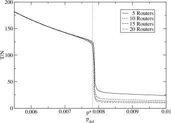
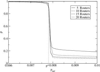
Figure 3: Left: Diagram of the mean travel times $T$ of data packets versus the probability $p_{\text{def}}$ of the last router for ($N=5,10,15,20$), $B=128$, and $p_{n}=0.2$. The mean travel times have been sampled over 500.000 updates after relaxation into the steady state. Right: Relation between the density $\rho$ of data packets and the probability $p_{\text{def}}$ of the last router. The parameters correspond to the ones used for the left diagram.

Varying $p_{\text{def}}$, computer simulations reveal the existence of two phases which can be distinguished by the behaviour of the travel times and the average density in the system (Fig. 3). The travel times are obtained from the simulations by summing up the waiting times $\tau_{i,n}$ of every single data packet $i$ in the routers along the path: $T_{i}=\sum_{n=1}^{N}\tau_{i,n}$. For a free flow system the mean waiting time for an arbitrary data packet in router $n$ can be estimated by

$$\tau_{n}=\sum_{t=0}^{\infty}tp_{n}(1-p_{n})^{t-1}=\frac{1}{p_{n}}.$$ (2)

The behaviour of the system is determined by the relation between $p_{\text{def}}$ and $p^{*}$ where $p^{*}$ corresponds to the point of maximum bulk flow. A simple estimation for $p^{*}$ is

$$p^{*}=\frac{j_{\text{in}}}{B_{\text{def}}}=\frac{1}{B},$$ (3)

i.e., for $p_{\text{def}}=p^{*}$ the inflow is equal to the mean maximum flow $p_{\text{def}}B_{\text{def}}$ through the last router.

For moving probabilities $p_{\text{def}}>p^{*}$ the maximum flow through the bottleneck is higher than the inflow $j_{\text{in}}$. In this free flow system the mean travel time only depends on the average capacity of each single router and can be described by

$$T_{\text{free}}=\sum_{n=1}^{N}\tau_{n}=\sum_{n=1}^{N}\frac{1}{p_{n}}=\sum_{n=1}^{N-1}\frac{1}{p_{n}}+\frac{1}{p_{\text{def}}}.$$ (4)

For lower moving probabilities ($p_{\text{def}}<p^{*}$) the mean flow through the bottleneck is lower than the inflow $j_{\text{in}}$ and the system gets jammed. In the jammed state, the maximum system flow is determined by the maximum capacity of the bottleneck. Data packets can only move to the next router when a data packet left it a time step before. This means that the mean travel time through the system is given by

$$T_{\text{jam}}=\frac{N}{p_{\text{def}}}.$$ (5)

For $p_{\text{def}}\approx p^{*}$ the mean flow through the bottleneck is equal to the inflow $j_{\text{in}}$ which means that the system operates at its maximum capacity. Simulations show that (4) and (5) are in excellent agreement with the results from Fig. 3.

The existence of two well defined regimes in the presence of a defect router $p_{\text{def}}$ is also confirmed by measurements of the mean density $\rho$ of the system (see Fig. 3) which is defined by $\rho=\sum_{n=1}^{N}\frac{Z_{n}}{B}$. In Fig. 3 one can distinguish a free flow state with low density for $p_{\text{def}}>p^{*}$ and a jammed state with high density for $p_{\text{def}}<p^{*}$ in agreement with the results for the travel time.

To compare the simulation results with empirical travel times from ping experiments, we investigated the statistics in the jammed and the free flow regime as well as in the transition region between these two regimes at $p_{\text{def}}=p^{*}$. Therefore we generated the power spectra of the travel times and analysed the spectral density. The left part of Fig. 4 shows the power spectrum of a free flow system ($p_{\text{def}}\gg p^{*}=1/B$). White noise is found for the whole frequency range. This means that correlations in the travel times of the data packets are negligible small. The data packets move with probability $p_{n}$ from one router to the next one without any limitation caused by the buffer restrictions. In contrast, jammed systems ($p_{\text{def}}\ll p^{*}$) show a algebraic decay with an approximately $1/f^{1/2}$ dependence at low frequencies (see right part of Fig. 4). Considering the occupancy of the buffer as a time dependent variable, the interval distribution of one jammed buffer corresponds to the first recurrence time in the random walk problem. Such a system then shows $1/f^{1/2}$-noise in the power spectrum and white noise at higher frequencies [2]. In the transition regime in the vicinity of $p^{*}$ the power spectra of the travel times show characteristic $1/f$-noise (see Fig. 5) at low frequencies (long range correlations, critical behaviour). All of the above findings of the statistical analysis of travel times generated by simulations of our simple model are in full agreement with the characteristic properties of measurements of ping time series in the Internet [2, 4].

Figure 4: Left: Power spectrum of a free flow system showing white noise ($N=15$, $B=128$, $p=0.2$, and $p_{\text{def}}=0.1$). Right: Power spectrum of a jammed system with $1/f^{1/2}$-noise at low and white noise at high frequencies ($N=15$, $B=128$, $p=0.2$, and $p_{\text{def}}=0.003$).

Figure 5: Power spectrum of a system at critical load ($N=15$, $B=128$, $p=0.2$, and $p_{\text{def}}=0.788$). One finds $1/f$-noise at low frequencies and white noise at high frequencies.

4 Discussion

We have introduced a simple cellular automaton model for the Internet data packet transport along a fixed path in the Internet. It is an asymmetric exclusion process where occupation of sites (buffers) by more than one particle (data packet) is allowed. Computer simulations have revealed the occurrence of a jammed and free flow phase in the presence of a slow router. To compare our model with real Internet data we focused on the dynamic behaviour of the travel times and their correlations. The analysis of travel times shows the typical power spectra of real Internet traffic in the two regimes, i.e., white noise for free flow and $1/f^{1/2}$ for the jammed system. In the transition regime between these two phases the model shows a characteristic $1/f$-noise.
In this work we focused on the effects due to one slow router in a fixed packet transport path, i.e., $p_{\text{def}}$. The influence of other parameters, e.g., $j_{\text{in}}$, $B_{\text{def}}$, $p_{n}$, etc., has been investigated in [4]. The results will be reported elsewhere. Future work should characterise the transition in more detail. In order to simulate the behaviour of networks where the nodes act as source and destination hosts the model has to be extended to two dimensions. However, our investigations indicate that many of the statistical properties of Internet traffic can already be understood by the simple one-dimensional model.

References

- [1] I. Csabai: J. Phys. A27, 417 (1994).
- [2] M. Takayasu, H. Takayasu: Physica A233, 924 (1996)
- [3] M. Takayasu, H. Takayasu, K. Fukuda: Physica A274, 144 (1999); Physica A277, 248 (2000).
- [4] T. Huisinga: Diploma Thesis, Duisburg University (2000).
- [5] W.E. Leland, M.S. Taqqu, W. Willinger, D.V. Willson: IEEE/ACM Trans. Networking 2, 1 (1994).
- [6] W. Willinger, M.S. Taqqu, R. Sherman, D.V. Wilson: IEEE/ACM Trans. Networking 5, 71 (1997).
- [7] B.A. Huberman, R.M. Lukose: Science 277, 535 (1997).
- [8] M. Takayasu, A.Yu. Tretyakov, K. Fukuda, H. Takayasu: in Traffic and Granular Flow ’97, edited by M. Schreckenberg and D. E. Wolf, p. 57 (Springer, 1998).
- [9] H. Hinrichsen: Adv. Phys. 49, 815 (2000).
- [10] J. Yuan, Y. Ren, X. Shan: Phys. Rev. E61, 1067 (2000).
- [11] K. Nagel, M. Schreckenberg: J. Phys. I France 2, 2221 (1992).
- [12] D. Chowdhury, L. Santen, A. Schadschneider: Phys. Rep. 329, 199 (2000), and references therein.
- [13] T. Ohira, R. Sawatari: Phys. Rev. E58, 193 (1998).
- [14] N. Vandewalle, D. Strivay, H.P. Garnir, M. Ausloos: in Traffic and Granular Flow ’97, edited by M. Schreckenberg and D.E. Wolf p. 75 (Springer, 1998).
- [15] G.M. Schütz, in: Phase Transitions and Critical Phenomena, Vol. 19, edited by C. Domb and J.L. Lebowitz (Academic Press, 2000), and references therein.
- [16] J. Krug: Phys. Rev. Lett. 67, 1882 (1991).