A Measure of data-collapse for scaling

Abstract

Data-collapse is a way of establishing scaling and extracting associated exponents in problems showing self-similar or self-affine characteristics as e.g. in equilibrium or non-equilibrium phase transitions, in critical phases, in dynamics of complex systems and many others. We propose a measure to quantify the nature of data collapse. Via a minimization of this measure, the exponents and their error-bars can be obtained. The procedure is illustrated by considering finite-size-scaling near phase transitions and quite strikingly recovering the exact exponents.

Scaling, especially finite size scaling (FSS), has emerged as an important framework for understanding and analyzing problems involving diverging length scales. Such problems abound in condensed matter, high energy and nuclear physics, equilibrium and non-equilibrium situations, thermal and non-thermal problems, and many more. The operational definition of scaling is this: A quantity $m(t,L)$ depending on two variables, $t$ and $L$, is considered to have scaling if it can be expressed as

$$m(t,L)=L^{d}f(t/L^{c}).$$ (1)

Depending on the nature of the problem of interest, $m$ may refer to magnetization, specific heat, size or some other characteristic of a polymer, width of a growing or fluctuating surface etc. Eq. 1 is the FSS form if $L$ is a linear dimension of the system and $t$ is any other variable, could even be time in dynamics. In the thermodynamic limit of infinite-sized systems, such a scaling would have $t$ and $L$ representing two thermodynamic parameters like magnetic field, pressure, chemical potential etc or one could be time. If $L$ is a length scale, then $d$ would look like the dimension of this quantity $m$, and $c$ of variable $t$. In fluctuation-dominated cases, it is generally a rule, rather than an exception, that $d$ and $c$ assume nontrivial values, different from what one expects from a dimensional analysis. The exponents and the scaling function $f(x)$ then characterize the behavior of the system. The fact that two completely independent variables (both conceptually and as controlled in experiments) combine in a nontrivial way to form a single one leads to an enormous simplification in the description of the phenomenon. This underlies the importance of scaling.

A quantitative way of showing scaling is data-collapse (also called scaling plot) that goes back to the original observation of Rushbrooke that the coexistence curves for many simple systems could be made to fall on a single curve[3]. For example, the values of $m(t,L)$ (Eq. 1) for various $t$ and $L$ can be made to collapse on a single curve if $mL^{-d}$ is plotted against $tL^{-c}$. The method of data-collapse therefore comes as a powerful means of establishing scaling. It is in fact now used extensively to analyze and extract exponents especially from numerical simulations. Given the importance of scaling in wide varieties of problems, it is imperative to have an appropriate measure to determine the “goodness of collapse” - not to be left to the eyes of the beholder.

In this paper, we propose a measure that can be used to quantify “collapse”. This measure can be used, via a minimization principle, for an automatic search for the exponents thereby removing the subjectiveness of the approach. To show the power of the method and the measure, we use it for two exactly known cases, namely the finite-size-scaling of the specific heat for (1) the one-dimensional ferro-electric six vertex model[4] showing a first order transition [5], and (2) the Kasteleyn dimer model[6] exhibiting the continuous anisotropic Pokrovsky-Talapov transition[7, 8]. In addition, to show the usefulness of the method in case of noisy data as expected in any numerical simulation, we consider the one-dimensional case with extra Gaussian noise added (by hand). It is worth emphasizing that the proposed procedure, without any bias, recovered the exactly known exponents from the specific heat data for finite systems.

If the scaling function $f(x)$ of Eq. 1 is known, then the sum of residuals

$$R=\frac{1}{N}\ \sum\mid L^{-d}\ m-f(t/L^{c})\mid,$$ (2)

where the sum is over all the data points, is minimum for the right choice of $(d,c)$. In absence of any statistical or systematic error, the minimum value is zero.

However in most situations the function itself is not known but is generally an analytic function. In case of a perfect collapse, any one of the sets (say set $p$) can be used for $f(x)$. An interpolation scheme can then be used to estimate the values for other sets in the overlapping regions . The residuals are then calculated. Since this can be done for any set as the basis, we repeat the procedure for all sets. Let the tabulated values of $m$ and $t$ be denoted by $m_{ij},t_{ij}$ ( $i$th value of $t$ for the $j$th set of $L$ (i.e.$L=L_{j}$ for set $j$ )). We now define a quantity $P_{b}$,

$$P_{b}=\left[\frac{1}{{\cal N}_{\rm over}}\ \sum_{p}\ \sum_{j\neq p}\ \sum_{i,{\rm over}}\mid L_{j}^{-d}\ m_{i,j}-{\cal E}_{p}(L_{j}^{-c}\,t_{ij})\mid^{q}\right]^{{}^{1/q}},$$ (3)

where ${\cal E}_{p}(x)$ is the interpolating function based on the values of set $p$ bracketing the argument in question (of set $j$). The innermost sum over $i$ is done only for overlapping points (denoted by the “$i$, over”), ${\cal N}_{\rm over}$ being the number of pairs. Though defined with a general $q$, we use $q=1$. For ${\cal E}_{p}(x)$, a 4-point polynomial interpolation can be used and if any complex singularity is suspected a rational approximation may be used. Extrapolations are avoided. The minimum of this function $P_{b}$ is zero[9] and is achievable in the ideal case of perfect collapse with correct values of $(d,c)$, i.e.,

$$P_{b}\geq P_{b}|_{\rm abs\ min}=0$$ (4)

This inequality can then be exploited and a minimization of $P_{b}$ over $(d,c)$ can be used to extract the optimal values of the parameters.

In addition to the values of the exponents, estimates of errors can be obtained from the width of the minimum. A simple approach is to take the quadratic part in the individual directions along the (d,c) plane. From an expansion of $\ln P_{b}$ around the minimum at $(d_{0},c_{0})$, the width is estimated as

$$\Delta d=\eta d_{0}\left[2\ln\frac{P_{b}(d_{0}\pm\eta d_{0},c_{0})}{P_{b}(d_{0},c_{0})}\right]^{{}^{-1/2}},$$ (6)

and

$$\Delta c=\eta c_{0}\left[2\ln\frac{P_{b}(d_{0},c_{0}\pm\eta c_{0})}{P_{b}(d_{0},c_{0})}\right]^{{}^{-1/2}},$$ (7)

for a given $\eta$. Choosing $\eta=1\%$, the final estimate for the exponents would be $d_{0}\pm\Delta d,c_{0}\pm\Delta c$ with the error bar reflecting the width of the minimum at $1\%$ level.

We now use the proposed method for different test cases. In order to implement the program[10], we have used the routines of numerical recipes[11]. To calculate $P_{b}$, POLINT or RATINT has been used for interpolation with HUNT to place a point in the table. For minimization, AMOEBA has been used thrice to locate the minimum, each time using the current estimates to generate a new triangle enclosing the minimum. In the examples given below, there was no need for more sophisticated minimization routines, which could be needed in case of subtle crossover behaviors or with nearby minima.

Let us first consider the one-dimensional six-vertex model which shows a first-order transition[5]. With the partition function $Z=2+(2x)^{N}$ for $N$ sites with $x=\exp(-\epsilon/k_{B}T)$ as the Boltzmann factor, $\epsilon$ being the energy of the high-energy vertices, $T$ the temperature and $k_{B}$ the Boltzmann factor, the specific heat can be computed exactly. The first-order transition is at $x=1/2$, for $N\rightarrow\infty$, with a $\delta$-function jump in specific heat. The $N$-dependent specific heat (per site),$c_{N}$, is given by[5]

$$c_{N}=k_{B}(\ln x)^{2}2N\frac{(2x)^{N}}{[2+(2x)^{N}]^{2}},$$ (8)

which for large $N$ and small $t=1-2x$ has the scaling form of Eq. 1 with $d=1$, $c=-1$ and

$$f(z)=k_{B}(\ln 2)^{2}2\frac{e^{z}}{(2+e^{z})^{2}}.$$ (9)

From the exact formula, Eq. 8, data were generated for $N=10,30,50,70$ and $90$, for various values of temperatures. A minimization of $P_{b}$ gave us the estimate $d=.997\pm 0.04,c=.98\pm.06$, with $P_{b}=0.56881E-01$. The exponents are very close to the exact ones. The error-bars or the width of the minimum is to be interpreted as an indication of the presence of non-scaling corrections. To test this, we have generated data from the exact scaling function of Eq. 9. An unbiased minimization of $P_{b}$ then gave $d=1\pm 0.004,c=-1\pm 0.004$ with $P_{b}=0.34876E-03$. The smallness of the residue and of the errors (or the width of the minimum) represents a good data collapse. The nature of the data-collapse for both the cases is shown in Fig. 1.

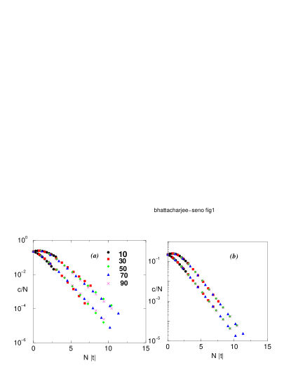
FIG. 1.: The collapse of the specific heat for the 1-d vertex model as calculated from Eq. 8 [Fig.(a)] and from Eq. 9 [Fig. (b)]. The x-axis in both the plots is $\mid t\mid/N^{c}$. The upper (lower) branch is for $t>0$ ($t<0$). For both, the exact values $d=1,c=-1$ are used.

A similar minimization of $P_{b}$ was carried out for the two-dimensional Kasteleyn dimer model ( also isomorphic to a two-dimensional 5 vertex model). This is an exactly solvable lattice model of the continuous anisotropic Pokrovsky-Talapov transition for surfaces, and shows a square-root singularity for specific heat with different correlations lengths in the two directions[8, 12]. The specific heat for lattices of size $M$ along the direction of the “walls” and infinite in the transverse direction is known exactly and its finite size scaling form has been discussed in Ref [8]. Using the following formula for the specific heat per site $c_{M}$

$$\frac{c_{M}}{k_{B}a}=M\int_{0}^{2\pi}\ \frac{(2x\cos\phi)^{M}}{[1+(2x\cos\phi)^{M}]^{2}}\ d\phi,$$ (10)

specific heats data were generated for $M=10,30,50,70$ and $90$. In this formula, a few unimportant factors are put under $a$ and not explicitly shown. The critical point is at $x=1/2$. A minimization of $P_{b}$ gave $d=.5\pm 0.03,c=-.945\pm.02$ to be compared with the exact values $d=.5,c=-1$. The residue factor is $P_{b}=0.12424E-01$. The importance of correction terms are clear from Fig. 5 of Ref. [8], and in our approach it gets reflected in the not too small value of $P_{b}$.

The function $P_{b}$ for $q=1$ for the above two-dimensional problem is shown as a surface plot over the $(d,c)$ plane in Fig. 1. The sharpness of the minimum is note-worthy. In both the examples considered, the performance of the method is remarkable.

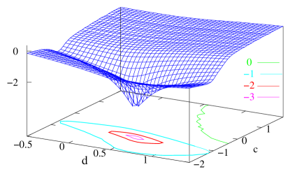
FIG. 2.: The residue $P_{b}$ with $q=1$ is shown over the $(d,c)$ plane. The $z$-axis is in log scale. A few contours of constant $\ln(P_{b})$ are shown in different colors on the $(d,c)$ plane.

The last example we consider is the set of noisy data[13] where $c$ is calculated from Eq. 9 and Gaussian noise was added to it so that $c_{N,\eta}=|c_{N}\ (1+A\eta)|$ where $\eta$ is a Gaussian deviate and $A$ is the amplitude of the noise added. The absolute value is taken to keep $c_{n}$ positive. The values of the exponents are found to be insensitive to $A$ for $A<0.1$ and starts changing for higher values of $A$. In Fig. 3 we show $P_{b}$ against $A$. The larger values of $P_{b}$ for larger $A$ is a sign of poor collapse, as one finds by direct plotting with the estimated values or exact values.

FIG. 3.: Noisy data. Plots of $P_{b}$ against $A$. Inset shows the estimated value of $d$ as a function of $A$.

To summarize, we have proposed a measure to quantify the nature of data collapse in any scaling analysis of the form given by Eq. (1). This measure can be used for an automated search for the exponents. The method is quite general and even-though we formulated it in terms of power-laws as in Eq. 1, it can very easily be adopted to other forms of scaling[14]. We conclude that the subjectiveness of data-collapse can be removed and $P_{b}$ could be used as a quantitative measure to test or compare “goodness of collapse” in any scaling analysis.

We acknowledge financial support from MURST(COFIN-99).

REFERENCES

- [1] email:somen@iopb.res.in
- [2] email:flavio.seno@pd.infn.it
- [3] H. E. Stanley, Rev. Mod. Phys. 71, S358 (1999).
- [4] E. Lieb and F. Y. Wu in Phase transitions and critical phenomena, Vol. 1, ed by C. Domb and M. Green (Academic, 1971).
- [5] S. M. Bhattacharjee, cond-mat/0011011 .
- [6] P. W. Kasteleyn, J. Math. Phys. 4, 287 (1963).
- [7] V. L. Pokrovksy and A. L. Talapov, Phys. Rev. Lett. 42, 65 (1979). J. F. Nagle, Phys. Rev. Lett. 34, 1150 (1975).
- [8] S. M. Bhattacharjee and J. F. Nagle, Phys. Rev. A31, 3199 (1985).
- [9] Pathological cases of no overlap are avoided.
- [10] This program is available on request from the authors. It is flexible enough that the Numerical Recipes[11] routines could be replaced by any other suitable package.
- [11] W. H. Press, S. A. Teukolsky, W. T. Vetterling, B. P. Flannery, Numerical recipes in FORTRAN 77, Cambridge University Press 1992.
- [12] Along the direction of the “walls” the bulk length-scale exponent is while in the transverse direction .
- [13] For analysis of noisy series, see, e.g., R. Dekeyser, F. Iglói, F. Mallezie, and F. Seno, Phys. Rev. A 42, 1923 (1990).
- [14] . For example, when tested on a log-type singularity as one finds for the specific heat in the two-dimensional Ising model, the method does not give a good collapse with power laws, but yields the correct results when the power-laws are changed to log’s.