[

Exact Bond-Located Spin Ground State in the Hubbard Chain with Off-Diagonal Coulomb Interactions

Abstract

We show the existence of an exact ground state in certain parameter regimes of one-dimensional half-filled extended Hubbard model with site-off-diagonal interactions. In this ground state, the bond-located spin correlation exhibits a long-range order. In the case when the spin space is SU(2) symmetric, this ground state degenerates with higher spin states including a fully ferromagnetic state. We also discuss the relation between the exact bond-ordered ground state and the critical bond-spin-density-wave phase.

]

The Hubbard model is one of the generic models to describe interacting electrons in narrow-band systems [1]. The on-site repulsion of this model is due to the matrix elements of the Coulomb interaction corresponding to the on-site Wannier states, and the other matrix elements are neglected. The importance of the neglected nearest-neighbor exchange interactions was, however, stressed and discussed for stabilization of ferromagnetism or a dimerized state [2, 3].

Japaridze first discussed using the weak-coupling theory the possibility of the bond-spin-density-wave (BSDW) ground state connected with the site-off-diagonal nature of the pair-hopping term [4]. He introduced the BSDW order parameters ${\mbox{\boldmath$\cal O$}_{i}}=({\cal O}_{i}^{\mathstrut x},{\cal O}_{i}^{y},{\cal O}_{i}^{\mathstrut z})$:

$${\mbox{\boldmath$\cal O$}}_{i}={\textstyle\frac{1}{2}}(-1)^{i}\sum_{\sigma\sigma^{\prime}}(c_{i\sigma}^{\dagger}\mbox{\boldmath$\tau$}_{\sigma\sigma^{\prime}}^{\mathstrut}c_{i+1\sigma^{\prime}}^{\mathstrut}+{\rm h.c.})$$ (1)

with the Pauli matrices $\mbox{\boldmath$\tau$}=(\tau^{x},\tau^{y},\tau^{z})$, where the operator $c_{i\sigma}^{\dagger}$ ($c_{i\sigma}^{\mathstrut}$) creates (annihilates) an electron with spin $\sigma$ ($=\uparrow,\downarrow)$ at the $i$-th site. The $z$-component of these order parameters (BSDW-$z$) ${\cal O}_{i}^{z}$ describes a staggered magnetization with spins located on bonds between adjacent sites (see Fig. 1).

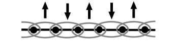
FIG. 1.: The BNéel state given by Eq. (16). The enclosed pairs of sites (gray ovals) indicate electron-hole dimers.

First in this Letter, we exactly demonstrate that the half-filled one-dimensional (1D) Hubbard model with site-off-diagonal interactions and a spin anisotropy has a doubly degenerate bond-ordered ground state in an intermediate coupling regime, using the optimal ground state approach [5, 6, 7, 8, 9]. This bond-ordered state is interpreted as a Néel state of bond-located spins, and the state realizes the fully BSDW long-range order with respect to the z-direction. For this reason we call the state the Bond-Néel (BNéel) state in the following. In this state there are no correlations with respect to both of site-located charge and spin density operators except for the nearest neighbor. The system possesses, therefore, charge and spin gaps between the ground state and excited states.

Next we consider a spin SU(2) symmetric case, and we show that the existence of the phase in which the BSDW correlation is dominant by using numerical methods as the level-crossing approach [10, 11]. The BSDW correlation shows a power-law decay at large distances and the system has a gapless spin excitation. This BSDW phase borders on the BNéel phase on the multicritical point. We discuss the relation between the BNéel state and the critical BSDW state.

We consider the 1D extended Hubbard model with on-site and nearest-neighbor interaction given by

$${\textstyle\frac{1}{2}}\sum_{ijkl}\sum_{\sigma\sigma^{\prime}}\langle{ij}|v_{\sigma\sigma^{\prime}}|{kl}\rangle c_{i\sigma}^{\dagger}c_{j\sigma^{\prime}}^{\dagger}c_{l\sigma^{\prime}}^{\mathstrut}c_{k\sigma}^{\mathstrut},$$

where the matrix elements with respect to on-site or nearest-neighbor only are nonzero. The Hamiltonian is ${\cal H}=\sum_{\langle{i,j}\rangle}h_{ij}$, where the local Hamiltonian $h_{ij}$ is given by

$$h_{ij} = \sum_{\sigma}(c_{i\sigma}^{\dagger}c_{j\sigma}^{\mathstrut}+{\rm h.c.})\bigl{[}-t+X(n_{i-\sigma}+n_{j-\sigma})\bigr{]}$$ (5)

$$\vphantom{\sum_{\sigma}}+{\textstyle\frac{1}{2}}U\bigl{[}(n_{i\uparrow}-{\textstyle\frac{1}{2}})(n_{i\downarrow}-{\textstyle\frac{1}{2}})+(n_{j\uparrow}-{\textstyle\frac{1}{2}})(n_{j\downarrow}-{\textstyle\frac{1}{2}})\bigr{]}$$

$${}+\sum_{\sigma\sigma^{\prime}}V_{\sigma\sigma^{\prime}}(n_{i\sigma}-{\textstyle\frac{1}{2}})(n_{j\sigma^{\prime}}-{\textstyle\frac{1}{2}})$$

$${}+{\textstyle\frac{1}{2}}W\sum_{\sigma\sigma^{\prime}}(c_{i\sigma}^{\dagger}c_{j\sigma}^{\mathstrut}+c_{j\sigma}^{\dagger}c_{i\sigma}^{\mathstrut})(c_{i\sigma^{\prime}}^{\dagger}c_{j\sigma^{\prime}}^{\mathstrut}+c_{j\sigma^{\prime}}^{\dagger}c_{i\sigma^{\prime}}^{\mathstrut}).$$

Here the summation is taken over pairs of neighboring sites $\langle{i,j}\rangle$, and the number operators is defined as $n_{i\sigma}=c_{i\sigma}^{\dagger}c_{i\sigma}^{\mathstrut}$. The first term in the Hamiltonian (5) is the single-particle hopping ($t$-term) including the bond-charge interaction $X=\langle{ii}|v_{\sigma\sigma^{\prime}}|{ij}\rangle$. The on-site coupling is $U=\langle{ii}|v_{\sigma,-\sigma}|{ii}\rangle$. Nearest-neighbor density interaction with opposite and parallel spins are parametrized by $V_{\sigma,-\sigma}=V_{\bot}=\langle{ij}|v_{\sigma,-\sigma}|{ij}\rangle$ and $V_{\sigma\sigma}=V_{\parallel}=\langle{ij}|v_{\sigma\sigma}|{ij}\rangle$, respectively. Here we introduce spin anisotropy due to some factors, such as the crystal structure and spin-orbit interaction. The bond-bond interaction is controlled by $W=\langle{ij}|v_{\sigma\sigma^{\prime}}|{ji}\rangle=\langle{ii}|v_{\sigma\sigma^{\prime}}|{jj}\rangle$.

Now let us show that the above Hamiltonian can be factorized in some parameter space. For this purpose, we introduce a local bond operator with spin $\sigma$ defined by

$$R_{ij}^{\sigma}(\lambda,\mu)=\lambda\,a_{ij\sigma}^{\dagger}a_{ij\sigma}^{\mathstrut}+\mu\,s_{ij\sigma}^{\mathstrut}s_{ij\sigma}^{\dagger},$$ (6)

where the operators $s_{ij\sigma}^{\dagger}$ and $a_{ij\sigma}^{\dagger}$ denote the symmetric and antisymmetric bond-creation operators, respectively: $s_{ij\sigma}^{\dagger}=\bigl{(}c_{i\sigma}^{\dagger}+c_{j\sigma}^{\dagger}\bigr{)}/\sqrt{2}$, $a_{ij\sigma}^{\dagger}=\bigl{(}c_{i\sigma}^{\dagger}-c_{j\sigma}^{\dagger}\bigr{)}/\sqrt{2}$. The bond operator $R_{ij}^{\sigma}(\lambda,\mu)^{\mathstrut}$ can be rewritten by using the operators $B_{ij}^{\sigma}=c_{i\sigma}^{\dagger}c_{j\sigma}^{\mathstrut}+{\rm h.c.}$ and $N_{ij}^{\sigma}=n_{i\sigma}+n_{j\sigma}$:

$$R_{ij}^{\sigma}(\lambda,\mu)=\frac{\lambda+\mu}{2}\bigl{(}1-B_{ij}^{\sigma}\bigr{)}+\frac{\lambda-\mu}{2}\bigl{(}N_{ij}^{\sigma}-1\bigr{)}.$$ (7)

The local Hamiltonian (5) can be written as follows:

$$h_{ij} = \vphantom{\frac{U}{2}}R_{ij}^{\uparrow}(\alpha,\beta)\,R_{ij}^{\downarrow}(\alpha^{\prime},\beta^{\prime})+R_{ij}^{\uparrow}(\lambda,\mu)\,R_{ij}^{\downarrow}(\lambda^{\prime},\mu^{\prime})$$ (10)

$${}+\sum_{\sigma\sigma^{\prime}}\tilde{V}_{\sigma\sigma^{\prime}}(n_{i\sigma}-{\textstyle\frac{1}{2}})(n_{j\sigma^{\prime}}-{\textstyle\frac{1}{2}})$$

$${}+(W+X-t)\sum_{\sigma}B_{ij}^{\sigma}+X(n_{i}+n_{j})-(t+X),$$

where $\tilde{V}_{\sigma\sigma}=V_{\parallel}-W$ and $\tilde{V}_{\sigma\sigma^{\prime}}=V_{\bot}-U/2$ ($\sigma\neq\sigma^{\prime}$). Here the parameters of operators $R_{ij}^{\sigma}$ in (10) are constrained to satisfy the relations:

$$2(\alpha\alpha^{\prime}+\lambda\lambda^{\prime}) = U+6W-4t,$$ (11)

$$2(\beta\beta^{\prime}+\mu\mu^{\prime}) = U-2W+4t,$$ (12)

$$2(\alpha\beta^{\prime}+\lambda\mu^{\prime}) = 2(\alpha^{\prime}\beta+\lambda^{\prime}\mu)=-U+2W.$$ (13)

When $\lambda,\mu\geq 0$, we see from the Eq. (6) that the bond operator is positive semidefinite: $\bigl{\langle}R_{ij}^{\sigma}(\lambda,\mu)\bigr{\rangle}\geq 0$. Then for $U=2V_{\bot}$, $W=V_{\parallel}=t-X$ the local operator ${\tilde{h}}_{ij}=h_{ij}-X(n_{i}+n_{j})+t+X$ is also positive semidefinite as long as $\alpha,\alpha^{\prime},\beta,\beta^{\prime},\lambda,\lambda^{\prime},\mu,\mu^{\prime}\geq 0$.

From these facts, we find that the energy of the global Hamiltonian ${\cal H}$ is bounded from below in the following regime:

$$U=2V_{\bot},\quad W=V_{\parallel}=t-X,$$ (14)

$$\max\{2W-4t,\ -6W+4t\}\leq U\leq 2W.$$ (15)

We denote the global Hamiltonian ${\cal H}$ in this regime as ${\cal H}_{\rm b}$. We impose the periodic boundary condition on the system and choose the number of lattice sites $L$ to be even in the following. The lower bound is given as $E_{\rm lower}=-(t+X)L+2XN$, where $N$ denotes the total number of electrons. To obtain an upper bound of the ground-state energy, we consider the following trial wave functions:

$$\bigl{|}\Psi_{0}^{\sigma}\bigr{\rangle}=\prod_{i\in\{{\rm odd}\}}s_{i,i+1,\sigma}^{\dagger}\prod_{j\in\{{\rm even}\}}s_{j,j+1,-\sigma}^{\dagger}|0\rangle,$$ (16)

where $|0\rangle$ denotes the vacuum. A schematic illustration of this state is given in Fig. 1. The state corresponds to a half-filled state with a density $N/L=1$. Since $R_{ij}^{\sigma}(\lambda,\mu)\,s_{ij\sigma}^{\dagger}|0\rangle=0$, the state $s_{ij\sigma}^{\dagger}|0\rangle$ is an eigenstate of the local Hamiltonian ${\tilde{h}}_{ij}$ with eigenvalue zero: ${\tilde{h}}_{ij}^{\mathstrut}s_{ij\sigma}^{\dagger}|0\rangle=0$. Rewriting the global Hamiltonian as ${\cal H}_{\rm b}=\sum_{\langle i,j\rangle}\bigl{[}\,{\tilde{h}}_{ij}+X(n_{i}+n_{j})-(t+X)\bigr{]}$, we can see that the state (16) is also an eigenstate:

$${\cal H}_{\rm b}\,\bigl{|}\Psi_{0}^{\sigma}\bigr{\rangle}=-(t-X)L\,\bigl{|}\Psi_{0}^{\sigma}\bigr{\rangle}.$$ (17)

This means that the ground-state energy is bounded from above at $E_{\rm upper}=-(t-X)L$. At half filling, therefore, the upper and lower bound coincide, and the eigenstate $\bigl{|}\Psi_{0}^{\sigma}\bigr{\rangle}$ is the ground state in the regime (15). The ground-state energy is given as $E=-(t-X)L$.

FIG. 2.: Energies in the $L=N=8$ system at $V=W=t$. In the region where the singlet excitation (dotted line) is lower than the triplet one, the spin excitation has a gap. The singlet-triplet level crossing point corresponds to the CDW-BSDW phase boundary.

When $U=2W\geq t$, the system is in the the regime (15), and the spin exchange interaction obtains the SU(2) symmetry, $V_{\parallel}=V_{\bot}=V$. Then the operators $S_{\rm tot}^{\alpha}=\sum_{i}S^{\alpha}_{i}$, $\alpha=+,-,z$ commute with the Hamiltonian. In this case, we can deduce that the ground state $\bigl{|}\Psi_{0}^{\sigma}\bigr{\rangle}$ and a fully polarized ferromagnetic (FM) state, $|{\rm FM}\rangle=\prod_{i}\,c_{i\uparrow}^{\dagger}\,|0\rangle$, are degenerate. Since $S_{\rm tot}^{+}\bigl{|}\Psi_{0}^{\sigma}\bigr{\rangle}$ does not vanish, the states

$$\biggl{|}{l_{1}\atop m_{1}}{l_{2}\atop m_{2}}{\dots\atop\dots}\biggr{\rangle}^{\sigma}=\prod_{k}\,\bigl{(}S_{\rm tot}^{+}\bigr{)}^{{l}_{k}}\bigl{(}S_{\rm tot}^{-}\bigr{)}^{{m}_{k}}\,\bigl{|}\Psi_{0}^{\sigma}\bigr{\rangle}$$ (18)

are also eigenstates with the lowest energy eigenvalue and with $S_{\rm tot}^{z}=\sum_{k}(l_{k}-m_{k})_{\mathstrut}$, ($|S_{\rm tot}^{z}|\leq L/2$) as long as $\bigl{|}{l_{1}\atop m_{1}}{l_{2}\atop m_{2}}{\dots\atop\dots}\,\bigr{\rangle}^{\mathstrut\sigma}_{\displaystyle\mathstrut}\neq 0$. These states, however, may not be linearly independent each other. The eigenstates of $\mbox{\boldmath$S$}_{\rm tot}^{2}$ with $S_{\rm tot}^{z}$ may be constructed by linear combinations of the states (18) with $S_{\rm tot}^{z}$. Then these $\mbox{\boldmath$S$}_{\rm tot}$ states $(|\mbox{\boldmath$S$}_{\rm tot}|\leq L/2)$ may degenerate. In Fig. 2 we show energies in the $L=8$ system at $W=V=t$ in Eq. (5) using the exact diagonalization. At the exactly solvable point ($U=2t$), all the lowest states with total spin $|\mbox{\boldmath$S$}_{\rm tot}|\leq L/2$ and the density $N/L=1$ degenerate.

For $V_{\bot}>V_{\parallel}$, i.e., $t\leq 2W<U$, the Hamiltonian can be expressed as

$${\cal H}={\cal H}_{\rm b}\bigr{|}_{U=2W}+\gamma\sum_{\langle i,j\rangle}\bigl{(}N_{ij}^{\uparrow}-1\bigr{)}\bigl{(}N_{ij}^{\downarrow}-1\bigr{)}$$ (19)

with $\gamma=U/2-W>0$. The ground state is the FM state, since $|{\rm FM}\rangle$ gives the lowest eigenvalue both of ${\cal H}_{\rm b}\bigr{|}_{U=2W}$ and $\sum_{\langle{i,j}\rangle}\bigl{(}N_{ij}^{\uparrow}-1\bigr{)}\bigl{(}N_{ij}^{\downarrow}-1\bigr{)}$. The system undergoes, therefore, a first-order phase transition at this level-crossing point $\gamma=0$. At $U=-2W=-2t$, $X=0$, the $\eta$-paring operator with momentum $\pi$, $\eta^{\dagger}=\sum_{j}(-1)^{j}c_{j\downarrow}^{\dagger}c_{j\uparrow}^{\dagger}$, commutes with the Hamiltonian. Therefore the $\eta$-paring state: $|\eta\rangle=(\eta^{\dagger})^{N/2}|0\rangle$ is also an exact ground state, which agrees with the result by de Boer and Schadschneider [6]. From the above discussion, we obtain the phase diagram of the model (5) as shown in Fig. 3.

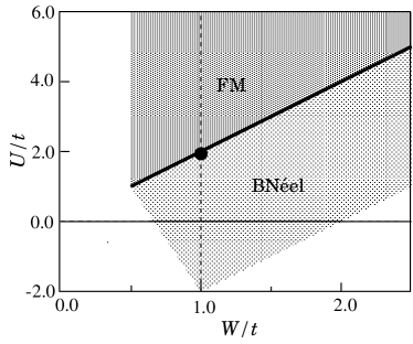
FIG. 3.: The phase diagram of the present model (5) in the $U$–$W$ plain. The parameters of the model are fixed as $U=2V_{\bot}$ and $W=V_{\parallel}=t-X$. The $X$-term vanishes on the vertical dotted line. The point denotes at $V_{\bot}=V_{\parallel},X=0$.

In order to analyze the properties of two ground states $\bigl{|}\Psi_{0}^{\uparrow}\bigr{\rangle}$ and $\bigl{|}\Psi_{0}^{\downarrow}\bigr{\rangle}$ in the regime (15), we introduce the matrix product representation [7, 8]. This is useful for calculating the ground state expectation values and correlation functions. First, we describe these states in terms of products of local $2\times 2$ matrices as,

$$\bigl{|}\Psi_{0}^{\sigma}\bigr{\rangle}=2^{-L/2}\>{\rm Tr}\>g_{1}^{\sigma}\otimes g_{2}^{-\sigma}\otimes\cdots\otimes g_{L-1}^{\sigma}\otimes g_{L}^{-\sigma},$$ (20)

where two matrices $g_{i}^{\sigma}$, $\sigma=\uparrow,\downarrow$, are given by

$$g_{i}^{\sigma}=\left(\begin{array}[]{cc}|{\sigma}\rangle_{i}&|2\rangle_{i}\\ |0\rangle_{i}&|{-\sigma}\rangle_{i}\end{array}\right).$$ (21)

Here $|\sigma\rangle_{i}=c_{i\sigma}^{\dagger}|0\rangle_{i}$, $|2\rangle_{i}=c_{i\uparrow}^{\dagger}c_{i\downarrow}^{\dagger}|0\rangle_{i}$, and $\otimes$ denotes the usual matrix multiplication of $2\times 2$ matrices with a tensor product of the matrix elements. Note that ${\tilde{h}}_{ij}\bigl{(}\,g_{i}^{\sigma}\otimes g_{j}^{-\sigma}\bigr{)}=0$. Next, we introduce $4\times 4$ transfer matrices: $G_{l_{1}l_{2}}^{\sigma\sigma^{\prime}}\equiv g_{n_{1}n_{2}}^{\sigma\dagger}\,g_{m_{1}m_{2}}^{\sigma^{\prime}}$, where $l_{k}=(n_{k},m_{k})$ and the indices correspond as $l_{k}=1,2,3,4\leftrightarrow(n_{k},m_{k})=(11),(12),(21),(22)$, respectively. Since the overlap between $\bigl{|}\Psi_{0}^{\downarrow}\bigr{\rangle}$ and $\bigl{|}\Psi_{0}^{\uparrow}\bigr{\rangle}$ for size $L$ is evaluated by $\bigl{\langle}\Psi_{0}^{\uparrow}\big{|}\Psi_{0}^{\downarrow}\bigr{\rangle}=2^{-L}\>{\rm Tr}\,(G^{\uparrow\downarrow})^{L}=4\!\cdot\!2^{-L}$, these two states are orthogonal in the limit $L\to\infty$. The ground state is, therefore, doubly degenerate, and the translational symmetry of the system is spontaneously broken except for $U=2W$.

The two-site correlation functions of operators $A_{1}$ at the 1st site and $B_{r}$ at the $r$-th site can be calculated by $\langle A_{1}B_{r}\rangle={\rm Tr}\,Z(A)\,G^{r-2}Z(B)\,G^{L-r}$ with $Z(A)=g^{\sigma\dagger}A\,g^{\sigma}$. Thus, the nearest neighbor correlations are obtained as follows, $\langle n_{i}n_{i+1}\rangle=2$, $\bigl{\langle}S_{i}^{z}S_{i+1}^{z}\bigr{\rangle}=-\frac{1}{4}$, and $\bigl{\langle}S_{i}^{+}S_{i+1}^{-}\bigr{\rangle}=0$. On the other hand, the two-point charge and spin correlation functions for $|i-j|\geq 2$ are $\langle n_{i}n_{j}\rangle-\langle n_{i}\rangle\langle n_{j}\rangle=0$ and $\bigl{\langle}S_{i}^{z}S_{j}^{z}\bigr{\rangle}=0$, respectively. These results indicate that there is a finite energy gap between the ground state and the excited states with respect to site-located charges and spins.

We can also obtain the bond-bond correlation functions as $\bigl{\langle}B^{\sigma}_{i,i+1}B^{\pm\sigma}_{j,j+1}\bigr{\rangle}=\bigl{(}1\pm(-1)^{|i-j|}\bigr{)}/2$, and thus we obtain the BSDW-$z$ correlation as $\bigl{\langle}{\cal O}_{i}^{z}{\cal O}_{j}^{z}\bigr{\rangle}=1$.

This result shows the existence of the BSDW-$z$ long-range order, and the expectation values of the BSDW-$z$ order parameter is given by $\bigl{\langle}{\cal O}_{i}^{z}\bigr{\rangle}=\pm 1$. Since $\{\,s_{i,i+1,\sigma}^{\mathstrut},a_{j,j+1,\sigma}^{\dagger}\}=0$, the expectation value of ${\cal O}_{i}^{z}$ can be expressed as $\bigl{\langle}{\cal O}_{i}^{z}\bigr{\rangle}=\bigl{\langle}(-1)^{i}(M_{i\uparrow}-M_{i\downarrow})\bigr{\rangle}$ with $M_{i\sigma}=s_{i,i+1,\sigma}^{\dagger}s_{i,i+1,\sigma}^{\mathstrut}$. Now we introduce a bond-spin vector operator given as $\mbox{\boldmath$T$}_{i}=\frac{1}{2}\sum_{\sigma\sigma^{\prime}}s_{i,i+1,\sigma}^{\dagger}\mbox{\boldmath$\tau$}_{\sigma\sigma^{\prime}}^{\mathstrut}s_{i,i+1,\sigma^{\prime}}^{\mathstrut}$. Then we have

$$\bigl{\langle}{\cal O}_{i}^{z}\bigr{\rangle}=2\bigl{\langle}(-1)^{i}\,T_{i}^{z}\bigr{\rangle}.$$ (22)

The BSDW-$z$ order just corresponds to the Néel order of the bond-located spins. Since the nearest-neighbor commutation relations of the bond-spin operators are different from those of the ordinary spin operators, the bond-spin and the spin operators are not exactly equivalent.

Next we discuss the relation between the BNéel and the BSDW states. As was discussed above, the BNéel state has both charge and spin gaps, whereas the BSDW state has gapped charge and gapless spin excitations [4]. Let us consider the Hamiltonian with an SU(2) symmetry in spin space given at $X=0$, $V_{\bot}=V_{\parallel}=V$ in Eq. (5). In this Hamiltonian, $\bigl{|}\Psi_{0}^{\sigma}\bigr{\rangle}$ gives an exact ground state when $U=2V=2W=2t$. There is large degeneracy in the ground state and the correlation function of the BNéel state are not reliable.

We show in Fig. 4 the phase diagram at $W/t=1$ in the $U$–$V$ plain, obtained by the exact diagonalization of the $L=12$ system. There appear BSDW, charge-density-wave (CDW), and FM phases. The CDW state has gaps both in charge and spin excitations, and shows a site-long-range order. The spin-gap transition occurs between the CDW-BSDW boundary. This transition point is obtained by the singlet-triplet level crossing in the excited states, which is justified by the conformal field theory [10]. On the other hand, the CDW-FM and the BSDW-FM transitions are of the first order, and their boundaries are determined by level crossing in the ground state [11]. Finite size effects in this analysis are small enough to get reliable results. The exact ground state appears just on the BSDW-FM boundary within the precision of the exact diagonalization.

FIG. 4.: The phase diagram of the model in the SU(2) symmetric case with $X=0,W=t$, obtained by the numerical data of the $L=12$ system. The wave function of Eq. (16) gives the exact ground state at $U=2V=2t$, which corresponds to the point indicated in Fig. 3.

As was shown in Fig. 2, at the exactly solvable point ($U=2t$), all the lowest states with the total spin $S_{\rm tot}$ ($S_{\rm tot}\leq L/2$) degenerate. From the above numerical and exact results, we conjecture that this total spin-$S_{\rm tot}$ states can be constructed by means of linear combinations of the states (18) and the singlet state in the constructed states corresponds to the BSDW state.

Finally, we comment on the relation between the present result and other works. Exact dimerized ground states in electron systems is discussed recently by Dmitriev et al. [12]. The dimer consists of up- and down-spin electrons, whereas our “dimer” given in Eq. (16) of an electron and a hole for each spin. Their results, therefore, do not contain a state with the staggered magnetization on the bonds. The ground state we have discussed is rather similar to the one which appears in a spin-$1/2$ two-leg ladder model [8] or in an orbitally degenerate spin chain [9] with the Jordan-Wigner transformation.

In summary, we have shown that a BNéel state with the BSDW order is the exact ground state in wide parameter space of the generalized Hubbard chain. In this state, both charge and spin excitations have gaps. In the case when SU(2) symmetry exists in the spin space, the ground state degenerates with higher spin states including the fully FM state. This BNéel phase adjoins the critical BSDW phase on the multicritical point. We expect that the relation between the BNéel and the BSDW states is analogous to the one between the Ising limit and the Heisenberg point in the spin-$1/2$ antiferromagnetic XXZ chain with respect to the low-energy spin excitations. Note, in the model (5), that the BNéel state appears when the spin anisotropy is XY-like, $V_{\bot}/W=V_{\bot}/V_{\parallel}<1$, contrary to the Néel state of the XXZ model.

REFERENCES

• [1] J. Hubbard, Proc. R. Soc. London A 276, 238 (1963); J. Kanamori, Prog. Theor. Phys. 30, 275 (1963); M. C. Gutzwiller, Phys. Rev. Lett. 20, 159 (1963).
• [2] J. E. Hirsch, Phys. Rev. B 40, 2354 (1989); 40, 9061 (1989); 43, 705 (1991); Physica B 163, 291 (1990).
• [3] D. K. Campbell, J. T. Gammel, and E. W. Loh, Jr., Phys. Rev. B 38, 12043 (1988); 42, 475 (1990).
• [4] G. I. Japaridze, Phys. Lett A 201, 239 (1995); G. I. Japaridze and E. Müller-Hartmann, J. Phys. Condens. Matter 9, 10509 (1997).
• [5] C. K. Majumder and D. K. Gohsh, J. Math. Phys. 10, 1388 (1969).
• [6] J. de Boer and A. Schadschneider, Phys. Rev. Lett. 75, 4298 (1995).
• [7] A. Klümper, A. Schadschneider, and J. Zittartz, Z. Phys. B 87, 281 (1992); Europhys. Lett. 24, 293 (1993).
• [8] A. K. Kolezhuk and H.-J. Mikeska, Phys. Rev. Lett. 80, 2709 (1998).
• [9] K. Itoh, J. Phys. Soc. Jpn. 68, 322 (1999).
• [10] M. Nakamura, J. Phys. Soc. Jpn. 68, 3123 (1999); Phys. Rev. B 61, 16377 (2000).
• [11] M. Nakamura, K. Itoh, and N. Muramoto, preprint (cond-mat/0003419).
• [12] D. V. Dmitriev, V. Ya. Krivnov, and A. A. Ovchinnikov, Phys. Rev. B 61, 14592 (2000); preprint (cond-mat/9911438).