Markov properties of high frequency exchange rate data

Abstract

We present a stochastic analysis of a data set consisiting of $10^{6}$ quotes of the US Doller - German Mark exchange rate. Evidence is given that the price changes $x(\tau)$ upon different delay times $\tau$ can be described as a Markov process evolving in $\tau$. Thus, the $\tau$-dependence of the probability density function (pdf) $p(x,\tau)$ on the delay time $\tau$ can be described by a Fokker-Planck equation, a gerneralized diffusion equation for $p(x,\tau)$. This equation is completely determined by two coefficients $D_{1}(x,\tau)$ and $D_{2}(x,\tau)$ (drift- and diffusion coefficient, respectively). We demonstrate how these coefficients can be estimated directly from the data without using any assumptions or models for the underlying stochastic process. Furthermore, it is shown that the solutions of the resulting Fokker-Planck equation describe the empirical pdfs correctly, including the pronounced tails.

keywords: econophysics, Markov processes, FX data
PACS: 02.50-r;05.10G;02.50.G

1 Introduction

Since L. Bachelier’s pioneering work dating back to 1900 [1], the complex statistical properties of economic systems have attracted the attention of many researchers and an extensive literature has evolved for modeling fluctuations of financial markets. Traditionally, fluctuations of financial assets were viewed and modeled as random variables. Well known examples are the ARCH-type models (see for example, [2, 3, 4]) and stochastic volatility (SV) models ([5, 6, 7]).

Since advances in computer technology have made high frequency data available, many physicists have joined the field adapting methods from statistical physics. One line of studies within econophysics focusses on the statistical properties of financial time series such as stock prices, stock market indices or currency exchange rates. Rather than comparing the predictions of models with the various aspects of emprical data (which is the traditional approach), physicists try to extract information about the stochastic processes governing financial markets from an analysis of emprical data. An overview of recent developments in this field can be found in references [9] , [10] and [11]. In spite of all the efforts spent, some of the most basic questions concerning the statistics of financial assets remain unsolved. In particular, the mechanism leading to the fat-tailed (leptokurtic) probability distributions of fluctuations on small time scales is still unknown. Compared to a Gaussian, the pdfs of those fluctuations express an unexpected high probability for large fluctuations (see figure 13). Quantifying the risks of such large fluctuations is of utmost importance for the risk management and the pricing of options.

Fluctuations of financial time series $y(t)$ are usually measured by means of returns, log-returns or, equivalently, by price increments. Here, we consider the statistics of the price increment $x(\tau)$ over a certain time scale $\tau$, which is defined as:

$$x(\tau)\;=\;y(t+\tau)-y(t).$$ (1)

We suppressed dependence of the price increment $x(\tau)$ on the time $t$ since we assume the underlying stochastic process to be stationary.

In a recent letter [12], we demonstrated that the mathematics of stochastic processes is a useful tool for empirical investigations of the time scale dependence of the proabability density function (pdf) $p(x,\tau)$ of the price increment $x$ on the time scale $\tau$. It was shown how the equations governing the underlying stochastic process can be extracted directly from the empirical data, provided that the price increment $x$ obeys a Markov process. In particular, it is possible to derive a partial differential equation, the Fokker-Planck equation, which describes the evolution of the pdf $p(x,\tau)$ in the scale variable $\tau$. Hence, the mathematics of Markov processes yields a complete description of the stochastic process underlying the evolution of the pdfs from Gaussian distributions at large scales $\tau$ to the leptokurtic pdfs at small scales.

Here, we extend our previous analysis presented in [12] considerably. We show how the existence of a Markov process can be checked empirically and how the Fokker-Planck equation can be calculated directly from the data. Furthermore, we show how multiplicative and additive noise sources interact leading to the leptokurtic distributions and volatility clustering of the exchange rates. Finally, our results are interpreted in the context of currently discussed features of financial time series. Since our method is not based on any models, we gain new insights into the mechanisms governing the statistics of economic systmes. In particular, we find new evidence for cascading processes in financial markets.

The paper is organized as follows. Section 2 is devoted to a brief summary of the most important notions and theorems on Markov processes and their application to the analysis of empirical data, while section 3 contains the main results of our analysis. We shall consider in detail a data set containing $10^{6}$ samples of the DM / US-Dollar exchange rate from the one-year period october ’92 to september ’93. An interpretation of our results is finally given in section 4.

2 Mathematics of Markov Processes

The following section briefly summarizes the notions and theorems which will be of importance for our statistical analysis. For further details on Markov processes we refer the reader to the references [14] and [15].

Fundamental quantities related to Markov processes are conditional probability density functions. Given the joint probability density $p(x_{1},\tau_{1};x_{2},\tau_{2})$ for finding the price increments $x_{1}\,(\,:=\,x(\tau_{1})\,)$ at a scale $\tau_{1}$ and $x_{2}$ at a scale $\tau_{2}$ with $\tau_{1}<\tau_{2}$, the conditional pdf $p(x_{1},\tau_{1}|x_{2},\tau_{2})$ is defined as:

$$p(x_{1},\tau_{1}|x_{2},\tau_{2})\;=\;\frac{p(x_{1},\tau_{1};x_{2},\tau_{2})}{p(x_{2},\tau_{2})}\;.$$ (2)

$p(x_{1},\tau_{1}|x_{2},\tau_{2})$ denotes the conditional probability density for the price increment $x_{1}$ at a scale $\tau_{1}$ given an increment $x_{2}$ at a scale $\tau_{2}$. It should be noted that the small scale $\tau_{1}$ lies within the larger scale $\tau_{2}$ (see equation (1): the increments $x_{1}$ and $x_{2}$ are calculated for the same time $t$).

Higher order conditional probability densities can be defined in an analogous way:

$$p(x_{1},\tau_{1}|x_{2},\tau_{2};...;x_{N},\tau_{N})\;=\;\frac{p(x_{1},\tau_{1};x_{2},\tau_{2};...;x_{N},\tau_{N})}{p(x_{2},\tau_{2};...;x_{N},\tau_{N})}\;.$$ (3)

Again, the smaller scales $\tau_{i}$ are nested inside the larger scales $\tau_{i+1}$ (with the common reference point $t$).

The stochastic process in $\tau$ is a Markov process, if the conditional probability densities fulfill the following relations:

$$p(x_{1},\tau_{1}|x_{2},\tau_{2};x_{3},\tau_{3};\ldots x_{N},\tau_{N})\; = \;p(x_{1},\tau_{1}|x_{2},\tau_{2})\;$$ (4)

with $\tau_{1}<\tau_{2}<\tau_{3}<\ldots<\tau_{N}$. As a consequence of (4), each N-point probability density $p(x_{1},\tau_{1};x_{2},\tau_{2};\ldots;x_{N},\tau_{N})$ can be determined as a product of conditional probability density functions:

$$p(x_{1},\tau_{1};...x_{N},\tau_{N})=p(x_{1},\tau_{1}|x_{2},\tau_{2})....p(x_{N-1},\tau_{N-1}|x_{N},\tau_{N})p(x_{N},\tau_{N})\;.$$ (5)

Equation (5) indicates the importance of the conditional pdf for Markov processes. Knowledge of $p(x,\tau|x_{0},\tau_{0})$ (for arbitrary scales $\tau$ and $\tau_{0}$ with $\tau<\tau_{0}$) is sufficient to generate the entire statistics of the price increment encoded in the N-point probability density $p(x_{1},\tau_{1};x_{2},\tau_{2};x_{3},\tau_{3};\ldots;x_{N},\tau_{N})$.

For Markov processes the conditional probability density fulfills a master equation which can be put into the form of a Kramers-Moyal expansion :

$$-\,\tau\,\frac{\partial}{\partial\tau}\,p(x,\tau|x_{0},\tau_{0})\;=\;\sum\limits_{k=1}^{\infty}\;\left(\,-\frac{\partial}{\partial x}\,\right)^{k}\,D_{k}(x,\tau)\,p(x,\tau|x_{0},\tau_{0}).$$ (6)

The Kramers-Moyal coefficients $D_{k}(x,\tau)$ are defined as the limit $\Delta\tau\rightarrow 0$ of the conditional moments $M_{k}(x,\tau,\Delta\tau)$:

$$D_{k}(x,\tau) \,=\, \lim_{\Delta\tau\rightarrow 0}\,M_{k}(x,\tau,\Delta\tau)\;,$$ (7)

$$M_{k}(x,\tau,\Delta\tau) \,=\, \frac{\tau}{k!\,\Delta\tau}\,\int\limits_{-\infty}^{+\infty}\,\left(\tilde{x}-x\right)^{k}\,p\left(\tilde{x},\tau-\Delta\tau|x,\tau\right)\,d\tilde{x}.$$ (8)

For a general stochastic process, all Kramers-Moyal coefficients are different from zero. According to Pawula’s theorem, however, the Kramers-Moyal expansion stops after the second term, provided that the fourth order coefficient $D_{4}(x,\tau)$ vanishes. In that case, the Kramers-Moyal expansion reduces to a Fokker-Planck equation (also known as the backwards or second Kolmogorov equation):

$$-\tau\frac{\partial}{\partial\tau}\,p(x,\tau|x_{0},\tau_{0})\;=\;\left\{\,-\frac{\partial}{\partial x}D_{1}(x,\tau)\,+\,\frac{\partial^{2}}{\partial x^{2}}D_{2}(x,\tau)\,\right\}p(x,\tau|x_{0},\tau_{0}).$$ (9)

$D_{1}$ is denoted as drift term, $D_{2}$ as diffusion term. The probability density $p(x,\tau)$ has to obey the same equation:

$$-\,\tau\,\frac{\partial}{\partial\tau}\,p(x,\tau)\;=\;\left\{\;-\,\frac{\partial}{\partial x}\,D_{1}(x,\tau)\;+\;\frac{\partial^{2}}{\partial x^{2}}\,D_{2}(x,\tau)\;\right\}\;p(x,\tau).$$ (10)

The Fokker-Planck equation describes the probability density function of a stochastic process generated by the Langevin equation (we use Itô’s definition)

$$-\tau\frac{\partial}{\partial\tau}x(\tau)=D_{1}(x,\tau)+\sqrt{D_{2}(x,\tau)}f(\tau)$$ (11)

where $f(\tau)$ is a Langevin force, i.e. $\delta$-correlated white noise with a gaussian distribution. Here, the increment $x(\tau)$ at a fixed time $t$ is generated by a stochastic process with respect to the continuous variable $\tau$. This kind of process expresses nothing else but a hierarchical, cascade-like structure connecting price increments on different time scales [16].

In the case that the random force $f(\tau)$ ist not Gaussian distributed, the Kramers-Moyal expansion does not reduce to the Fokker-Planck equation. From the more general Kramers-Moyal expansion (6), which is also valid for the probability density $p(x,\tau)$, differential equations for the n-th order moments can be derived. By multiplication with $x^{n}$ and integration with respect to $x$ we obtain:

$$-\tau\frac{\partial}{\partial\tau}\left<x^{n}(\tau)\right> \,=\, \sum\limits_{k=1}^{\infty}\,\left(-1\right)^{k}\,\int\limits_{-\infty}^{+\infty}\,x^{n}\,\left(\,\frac{\partial}{\partial x}\,\right)^{k}\,D_{k}(x,\tau)\,p(x,\tau)dv$$ (12)

$$\,=\, \sum\limits_{k=1}^{n}\,\frac{n!}{(n-k)!}\,\int\limits_{-\infty}^{+\infty}\,x^{n-k}\,D_{k}(x,\tau)\,p(x,\tau)dv\;.$$

$$\,=\, \sum\limits_{k=1}^{n}\,\frac{n!}{(n-k!)}\,\left<\,x^{n-k}\,D_{k}(x,\tau)\,\right>\;.$$

3 Data Analysis

The hypothesis concerning the Markovian properties of exchange rate data immediately fixes a framework for the analysis of the data. First, one has to give evidence of the Markovian properties according to equation (4). Secondly, the evolution of conditional probability densities $p(x_{1},\tau_{1}|x_{2},\tau_{2})$ has to be specified on the basis of the stochastic evolution equation, eq. (6). To this end, we have to determine the conditional moments $M_{k}(x,\tau,\Delta\tau)$ at different scales $\tau$ for various values of $\Delta\tau$.

Practically, it is only possible to evaluate the lowest order coefficients. Therefore, we shall restrict our analysis to the coefficients of order one, two, and four. Approximating the limit $\Delta\tau\rightarrow 0$, we obtain the Kramers-Moyal coefficients $D_{k}(x,\tau)$. If the fourth order coefficient vanishes, the evolution equation (6) takes the form of a Fokker-Planck equation, according to Pawula’s theorem. Since we consider a finite data set, we are not able to prove rigorously (in a mathematical sense) that $D_{4}$ is zero but can only give hints for the validity of the assumption that the conditional probability density obeys a Fokker-Planck equation.

In order to verify this assumption and our results for the Kramers-Moyal coefficients, we compare the numerical solutions of the Fokker-Planck equations (9) and (10) with the probability density functions determined directly from the data.

For the rest of the article, prices and price increments are given in units of the standard deviation $\sigma$ of $y(t)$. For the data set under consideration, $\sigma$ is $0.064DM$.

3.1 Data Processing

From the frequency spectrum (figure 1) of the exchange rate $y(t)$, it becomes evident that the data are dominated by white noise for high frequencies (above $\approx 10^{-2}Hz$), comparable to the noise affecting any physical measurement. The original signal $y(t)$ seems to be the sum of the underlying ”real” signal $s(t)$ and some additive white noise $n(t)$:

$$y(t)\;=\;s(t)+n(t).$$ (13)

The additive noise acts on the increments in a similar way (see equation (1)). Note that this noise differs from the dynamical noise of the Langevin equation (11). $n(t)$ can be regarded as some randomness which is added seperately to the dynamical stochastic cascade process. In physics this kind of noise is known as measurement noise [13].

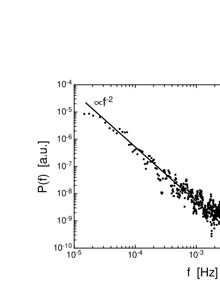
Figure 1: Frequency spectrum of the exchange rate data $y(t)$. For high frequencies the data are dominated by white noise.

As will be seen in capter 3.3, the existence of such an additive white noise dominating the small scales causes problems in our analysis, especially in the limit $\Delta\tau\rightarrow 0$ which has to be performed according to equation (7). In order to avoid these problems, we applied a low-pass filter to the data. Each value $y(t)$ was replaced by the weighted average of itself and its neighbouring data points, where the weighting function was chosen to be a gaussian centered at $t$ with a width of $44sec$. Figure 2 shows the result $s(t)$ of this procedure in comparison to the original data $y(t)$.

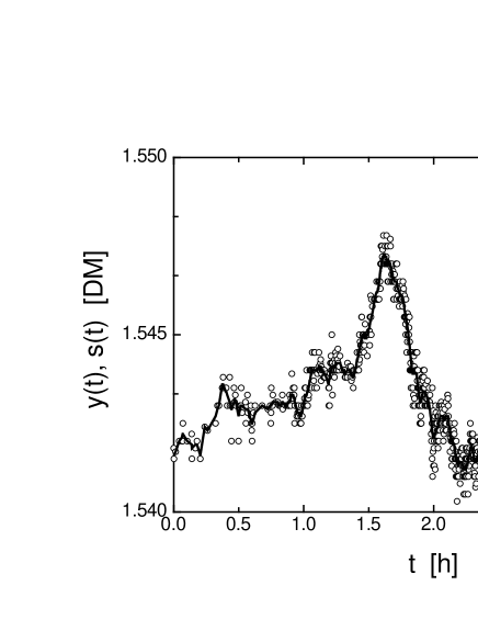
Figure 2: Samples of the time series of the original exchange rate data $y(t)$ (cirles) and the smoothed signal $s(t)$ (full line).

According to equation (13), we can extract the noise $n(t)$ by subtracting the smoothed signal from the original data $y(t)$. If the assumptions leading to equation (13) are correct and the algorithm used to smooth the data is an appropriate one, the extracted $n(t)$ should be white noise, i.e. it should be $\delta$-correlated with zero mean.

The ratio of the mean value $<n(t)>$ to the standard deviation $\sigma_{n}$ of $n(t)$ was found to be smaller than $8\cdot 10^{-5}$ ($\sigma_{n}=0.0003DM$). This result justifies the assumption of a zero mean for $n(t)$. The autocorrelation function $R_{n}(\tau)$ of $n(t)$ decreases from $1$ to $0.08$ within two seconds (see figure 3). Compared to the temporal resolution of the data (the smallest time step between two subsequent data points is two seconds), $R(\tau)$ indeed decreases rapidly. However, there appear to be small but significantly non-zero values for time delays $\tau\leq 2min$, indicating that the approximation of the ”real” signal $s(t)$ by the smoothed signal is insufficient. We therefore restrict our analysis to time delays $\tau$ larger than a certain elementary step $\tau_{min}$ which, from figure 3, we chose to be $4min$. In units of $\tau_{min}$, $R_{n}(\tau)$ can be considered to be $\delta$-correlated.

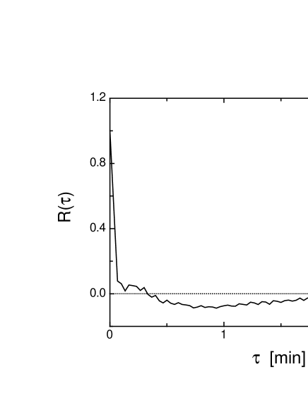
Figure 3: The autocorrelation function of the extracted additive noise $n(t)$.

Figure 4 finally compares the probability density functions of price increments $x(\tau)$ calculated from the original data $y(t)$ and the smoothed data $s(t)$. It becomes evident that the influence of the noise $n(t)$ is indeed restricted to small scales. For scales larger than $\tau=2\tau_{min}$ the pdfs are practically identical.

It may be worth to recall the result for fully developed turbulence, where a similar stochastic analysis was performed for velocity increments over space scales instead of price increments over time scales. In the case of turbulence, the Markovian properties were found to be valid only for (length-) scales and differences of scales larger than an elementary step size $l_{mar}$ [16]. But in contrast to the elementary step in turbulence which is a physical effect caused by the smoothing effects of viscous forces, the step $\tau_{min}$ used here for the analysis of financial data is due to the additional noise $n(t)$ as discussed above. We want to mention that it is not unusual to find such a ”cut off” at small scales for stochastic processes. For Brownian motion, the mean free path of molecules defines an elementary step size for the diffusion process in an analogous way.

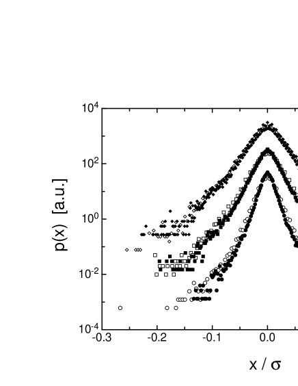
Figure 4: Pdfs of price increments $x(\tau)$ for $\tau=4min,8min$ and $15min$ (from bottom to top). The pdfs of $x$ were calculated from the smoothed data (full symbols) as well as from the original time series $y(t)$ (open symbols). Curves have been shifted in y-direction for clarity of presentation. Note that $\sigma$ ist not the respective standard deviation of each individual pdf, but the standard deviation of the whole data set $y(t)$.

For the rest of the article, the price increments $x_{i}(\tau_{i})$ are (unless it is mentioned explicitly) calculated from the smoothed data $s(t)$.

3.2 Markov Properties

Next, we give evidence that the Markovian property (4) holds. Strictly speaking, the relationships (4) have to be verified for all positive values of N as well as for each set of scales $\tau_{1},...,\tau_{N}$, a task, which is evidently impossible. However, the data set considered here consisting of $10^{6}$ samples allows to verify condition (4) for $N=3$:

$$p(x_{1},\tau_{1}|x_{2},\tau_{2};x_{3},\tau_{3})\;=\;p(x_{1},\tau_{1}|x_{2},\tau_{2}).$$ (14)

In figure 5, the contour plots of $p(x_{1},\tau_{1}|x_{2},\tau_{2})$ and $p(x_{1},\tau_{1}|x_{2},\tau_{2};x_{3}=0,\tau_{3})$ have been superposed for the scales $\tau_{1}=\tau_{min}=4min$, $\tau_{2}=2\tau_{min}$ and $\tau_{3}=3\tau_{min}$. The proximity of corresponding contour lines yields evidence for the validity of equation (14) for the chosen set of scales. Additionally, two cuts through the conditional probability densities are provided for fixed values of $x_{2}$.

Figure 5: (a): Contour plots of the conditional pdfs $p(x_{1},\tau_{1}|x_{2},\tau_{2})$ (dashed lines) and $p(x_{1},\tau_{1}|x_{2},\tau_{2};x_{3}=0,\tau_{3})$ (solid lines) for $\tau_{1}=\tau_{min}$, $\tau_{2}=2\tau_{min}$ and $\tau_{3}=3\tau_{min}$.
(b) and (c): Cuts through the conditional pdfs for $x_{2}=\pm 0.02\sigma$. Open symbols: $p(x_{1},\tau_{1}|x_{2},\tau_{2};x_{3}=0,\tau_{3})$, solid lines: $p(x_{1},\tau_{1}|x_{2},\tau_{2})$.

Figure 6 shows the same plots for a different set of scales: $\tau_{1}=1h$, $\tau_{2}=\tau_{1}+\tau_{min}$ and $\tau_{3}=\tau_{1}+2\tau_{min}$. Again, we find a good agreement between corresponding contour lines.

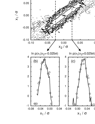
Figure 6: (a): Contour plots of the conditional pdfs $p(x_{1},\tau_{1}|x_{2},\tau_{2})$ (dashed lines) and $p(x_{1},\tau_{1}|x_{2},\tau_{2};x_{3}=0,\tau_{3})$ (solid lines) for $\tau_{1}=1h$, $\tau_{2}=\tau_{1}+\tau_{min}$ and $\tau_{3}=\tau_{1}+2\tau_{min}$.
(b) and (c): Cuts through the conditional pdfs for $x_{2}=\pm 0.025\sigma$. Open symbols: $p(x_{1},\tau_{1}|x_{2},\tau_{2};x_{3}=0,\tau_{3})$, solid lines: $p(x_{1},\tau_{1}|x_{2},\tau_{2})$.

Similar results were obtained for several other sets of scales chosen from the intervall $\tau_{min}\leq\tau_{1}\leq 2h$, with $\Delta\tau=\tau_{2}-\tau_{1}=\tau_{3}-\tau_{2}$ ranging from $\tau_{min}$ to $3\tau_{min}$.

Based on these result, we proceed with the well-founded assumption that the price increments of exchange rate data obey a Markov process for the range of scales under consideration, i.e. for scales and differences of scales larger than $\tau_{min}$.

3.3 Kramers-Moyal Coefficients

According to equations (2) and (8), the coefficients $M_{k}(x,\tau,\Delta\tau)$ can be calculated from the joint probability density functions. These joint pdfs $p(\tilde{x},\tau-\Delta\tau\,;\,x,\tau)$ are easily obtained from the data by counting the number $N(\tilde{x},x)$ of occurrences of the two increments $\tilde{x}$ and $x$.

According to equation (7), the limit $\Delta\tau\rightarrow 0$ has to be performed next in order to obtain the Kramers-Moyal coefficients. Figure 7 shows the coefficient $M_{2}(x,\tau,\Delta\tau)$ for exemplarily chosen fixed values of $x$ and $\tau$ as a function of $\Delta\tau$. Throughout the intervall $\tau_{min}\,\leq\,\Delta\tau\,\leq 3\tau_{min}$, the dependence of $M_{2}$ on $\Delta\tau$ turns out to be linear. For values of $\tau<\tau_{min}/2$, the values deviate from that linear behaviour. It is interesting to note that the range of scales where those deviations begin is identical with the range of scales for which the autocorrelation function of the reconstructed additive noise $n(t)$ has nonzero values (see figure 3). The limit $\Delta\tau\rightarrow 0$ is therefore performed by fitting a straight line to the $M_{n}$ in the intervall $\tau_{min}\leq\Delta\tau\leq 2\tau_{min}$, thus avoiding problems with the values for $\Delta\tau\leq\tau_{min}/2$ (see figure 7).

Figure 7 also displays the coefficient $M^{(y)}_{2}$, which is obtained when instead of the smoothed signal $s(t)$ the original data $y(t)$ is used to calculate the coefficients $M_{k}$. In the presence of additive white noise, the values of $M^{(y)}_{2}$ diverge as $\Delta\tau$ goes to zero. The limit $\Delta\tau\rightarrow 0$ can not be performed in this case. Since the coefficients $M_{k}$ are nothing but conditional moments of the increments (see equation (8)), the reason for this behaviour can easily be understood by expressing the second moment of the increment of $y(t)$ in terms of $s(t)$ and $n(t)$. Using equation (13), we obtain:

$$\left<\,\left(\,y(t+\tau)-y(t)\,\right)^{2}\,\right>\; = \;\left<\,\left(\,s(t+\tau)+n(t+\tau)-s(t+\tau)-n(t+\tau)\,\right)^{2}\,\right>$$ (15)

$$= \;\left<\,\left(\,s(t+\tau)-s(t)\,\right)^{2}\,\right>\;+\;2\left<\,n^{2}\,\right>.$$

Due to the additive nature of the white noise $n$, the additional constant term $2\left<\,n^{2}\,\right>$ arises which does not depend on the scale $\tau$. Similar terms also arise for the conditional moments $M_{k}$ when $y(t)$ is used instead of $s(t)$. Dividing the conditional moments of the increment by $\Delta\tau$ according to equation (8) thus leads to the diverging behaviour of $M_{k}^{(y)}$ in the limit $\Delta\tau\rightarrow 0$ as shown in figure 7.

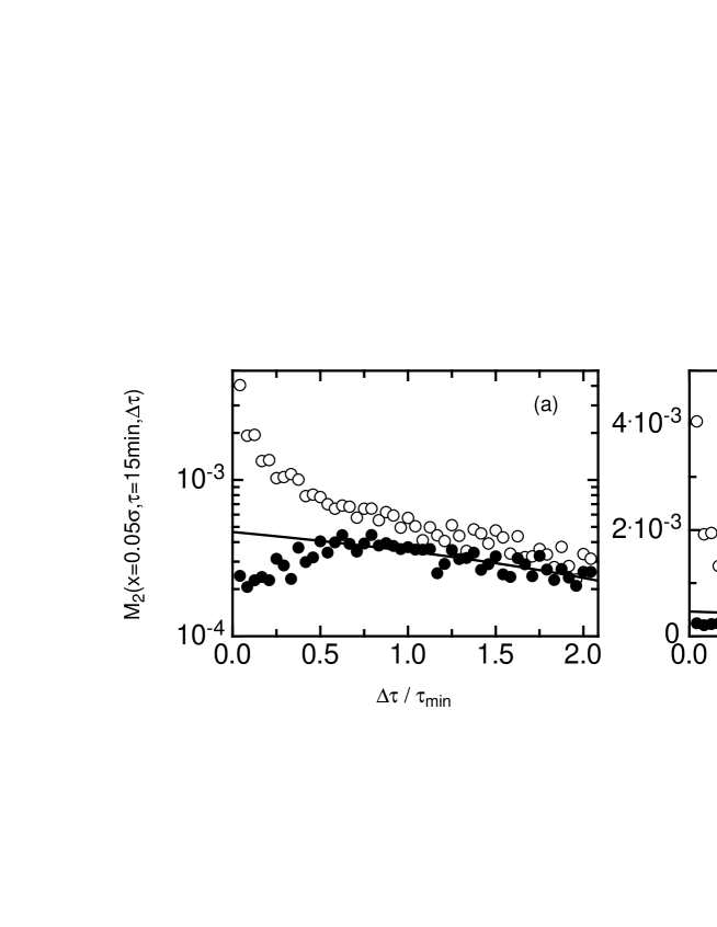
Figure 7: The coefficient $M_{2}(x,\tau,\Delta\tau)$ as a function of $\Delta\tau$ for $x=0.05\sigma$ and $\tau=15min$ (full circles). (a): logarithmic scale, (b): linear scale. For $\tau\geq\tau_{min}$, $M_{2}$ is a linear function of $\Delta\tau$ and can thus be extrapolated using a linear fit in the interval $\tau_{min}\leq\Delta\tau\leq 2\tau_{min}$ (full line). The open circles represent the results for $M_{2}$ for the same values of $x$ and $\tau$ when instead of the smoothed data $s(t)$ the original data $y(t)$ are used. The presence of additive white noise leads to diverging values for $M^{(y)}_{2}$ as $\Delta\tau$ goes to zero.

When the smoothed signal $s(t)$ is used to calculate the coefficients $M_{k}$, the linear dependence of $M_{k}(x,\tau,\Delta\tau)$ on $\Delta\tau$ is found to hold for $k=1,2$, several scales $\tau$ and all values of $x$. This enables us to calculate the coefficients $D_{1}(x,\tau)$ and $D_{2}(x,\tau)$ from the $M_{k}$ using the method of linear extrapolation described above. Figure 8 shows the results for $D_{1}$ and $D_{2}$ as a function of the price increment $x$ at several scales $\tau$. Both coefficients exhibit simple dependencies on the price increment. While $D_{1}$ is linear in $x$, $D_{2}$ can be approximated by a polynomial of degree two where the linear term is zero:

$$D_{1}(x,\tau) \;=\; -\,\gamma(\tau)\,x,$$

$$D_{2}(x,\tau) \;=\; \alpha(\tau)\;+\;\beta(\tau)\,x^{2}.$$ (16)

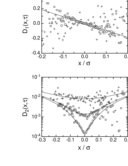
Figure 8: The coefficients $D_{1}$ (a) and $D_{2}$ (b) as functions of the price increment $x$ at scale $\tau=15min$ (circles), $\tau=2h$ (squares) and $\tau=12h$ (crosses). The lines represent the results for $D_{1}$ and $D_{2}$ obtained with the method described in section 3.5 (note the logarithmic presentation of $D_{2}$).

Equation (16) turns out to describe the dependencies of the coefficients $D_{k}$ on $x$ for all scales $\tau$ up to two hours (see figure 8). For larger scales, the statistics of the data are too poore to allow for a proper calculation of the coefficients $M_{k}$, which results in considerable scatter of $D_{1}$ and $D_{2}$ (as exemplarily shown for $\tau=12h$ in figure 8). Indeed, from the analogous analysis of turbulent data [16], we know that the conditional moments $M_{k}$ can be calculated properly only for scales $\tau$ with $\tau\leq 10^{-4}T$, where $T$ is the total length of the data set. With $T$ being one year for the data set considered here, we are thus restricted to scales smaller than one hour for a direct analysis of the Kramers-Moyal coefficients.

Fitting the $D_{k}(x,\tau)$ by straight lines and parabolas, respecitvely, therefore yields values for $\gamma(\tau)$, $\alpha(\tau)$ and $\beta(\tau)$ which scatter considerably and which do not exhibit a well defined functional dependence on the scale $\tau$. However, what can be concluded from the analysis of the coefficients $D_{k}$ is that the Kramers-Moyal coefficients are linear and quadratic functions of the price increment, respectively, with coefficients depending on the scale $\tau$.

3.4 The Fourth Order Coefficient

According to Pawula’s theorem, it is of importance to estimate the fourth order coefficient and to decide whether it may be neglected. Figure 9 shows the coefficient $M_{4}(x,\tau,\Delta\tau)$ for fixed values of $x$ and $\tau$ as a function of $\Delta\tau$. Again, we find a linear dependence of the coefficient on $\Delta\tau$ for $\Delta\tau\geq\tau_{min}$. But whereas $M_{2}(\Delta\tau)$ increases as $\Delta\tau$ goes to zero, $M_{4}$ decreases. Furthermore, the linear extrapolation yields a value for $D_{4}$ which is small compared to the values of $M_{4}$ for $\tau_{min}\leq\tau\leq 2\tau_{min}$. This is a first hint that $M_{4}$ tends to zero in the limit $\Delta\tau\rightarrow 0$.

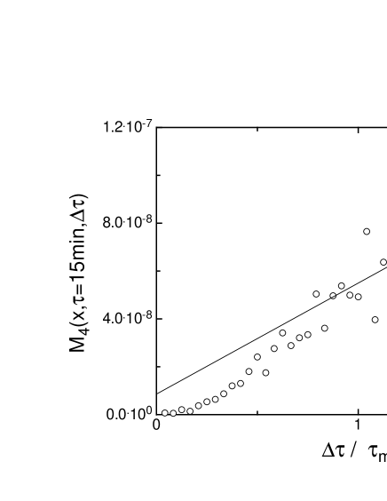
Figure 9: The coefficient $M_{4}(x,\tau,\Delta\tau)$ as a function of $\Delta\tau$ for $x=-0.05\sigma$ and $\tau=15min$ (circles).

Performing the limit $\Delta\tau\rightarrow 0$ for various values of $x$ using the linear extrapolation confirms the above results. We obtain positive as well as negative values for $D_{4}$, as shown in figure 10 for the scale $\tau=15min$. Since, by definition, $D_{4}$ is a positive quantity, this means that the data set allows to take $D_{4}$ to be zero.

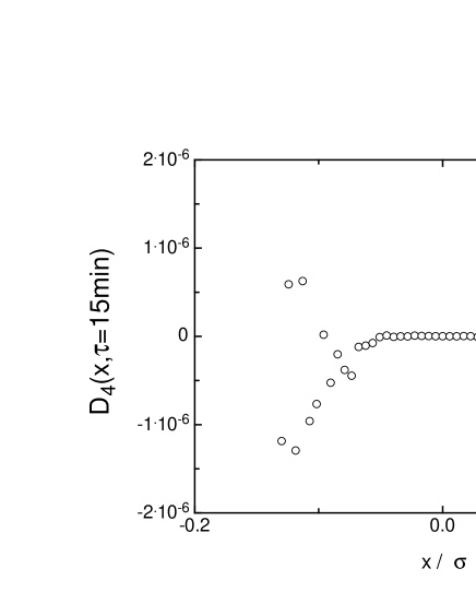
Figure 10: The fourth coefficient $D_{4}(x,\tau)$ as a function of $x$ for scale $\tau=15min$ (circles). The linear extrapolation yields positive as well as negative values for $D_{4}$.

Similar results were obtained for several scales $\tau\leq 2h$. Based on these results, we will proceed with the assumption that the fourth order coefficient $D_{4}$ vanishes, i.e. that Pawula’s theorem applies and that the stochastic process is described by the Fokker-Planck equation.

3.5 An Alternative Approach

Based on the results of the preceeding section, we will proceed with the assumption that the statistics of the price increment is governed by the Fokker-Planck euqation with coefficients $D_{1}$ and $D_{2}$ given by equation (16) and try to find estimates for the coefficients $\gamma$, $\alpha$ and $\beta$.

For the slope $\gamma(\tau)$ of $D_{1}$, such an estimate can be obtained from the conditional first order moment $T^{1}(\tau)=\left<\,x(\tau)\,|x_{0}(\tau_{0})\,\right>$ of the price increment. Multiplying the Fokker-Planck equation (9) with $x$, integrating with respect to $x$ and finally using the result (16) for $D_{1}$, an equation for $T^{1}(\tau)$ can be derived. The result is:

$$-\tau\frac{\partial}{\partial\tau}\,T^{1}(\tau)\; = -\,\gamma(\tau)\,T^{1}(\tau).$$ (17)

In deriving equation (17), it was assumed that $D_{2}(x,\tau)\,p(x,\tau|x_{0},\tau_{0})$ goes to zero for $|x|\rightarrow\infty$.

With the initial condition $T^{1}(\tau=\tau_{0})=\left<x(\tau=\tau_{0})|x_{0}(\tau_{0})\right>=x_{0}$, equation (17) is solved by:

$$T^{1}(\tau)\;=\;x_{0}\,\exp\left\{\,\int\limits_{\tau_{0}}^{\tau}\,\frac{\gamma(\tau^{\prime})}{\tau^{\prime}}\,d\tau^{\prime}\right\}.$$ (18)

If the conditional moment $T^{1}$ follows the simple prediction (18), this can be taken as a strong hint for the validity of the assumptions underlying the derivation (validity of the Fokker-Planck equation and linear dependence of $D_{1}$ on $x$). On the other hand, the simple dependence of $T^{1}(\tau)$ on $\gamma$ could also be used to measure the function $\gamma(\tau)$.

Figure 11 shows the conditional expectation values $T^{1}/x_{0}$ as a function of $\tau/\tau_{0}$ for scale $\tau_{0}=3h$ and several values of $x_{0}$. Indeed, as was expected from equation (18), $T^{1}$ divided by $x_{0}$ turns out to be an universal function of $\tau/\tau_{0}$. In particular, we do not find a systematic dependence on $x_{0}$.

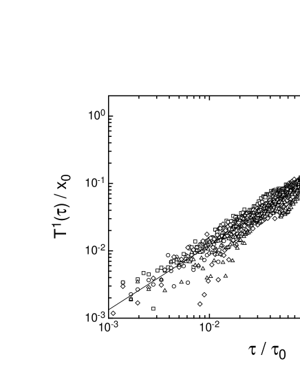
Figure 11: The conditional moment $T^{1}$ (divided by $x_{0}$) as a function of the time scale $\tau$ for $\tau_{0}=3h$, $x_{0}=-0.05\sigma$ (circles), $x_{0}=-0.025\sigma$ (squares), $x_{0}=0.05\sigma$ (diamonds) and $x_{0}=0.05\sigma$ (triangles). The straight line represents a power law fit to the data yielding a scaling exponent of $0.95$.

Furthermore, it is found that $T^{1}$ is well described by a power law in $\tau$, i.e.: $T^{1}\propto\tau^{c}$. It is easily seen that such a power law arises from equation (18) for the case that $\gamma(\tau)$ is constant:

$$T^{1}(\tau)\; = \;x_{0}\,\exp\left\{\,\int\limits_{\tau_{0}}^{\tau}\,\frac{\gamma}{\tau^{\prime}}\,d\tau^{\prime}\right\}\;=\;x_{0}\,\exp\left\{\,\gamma\ln\left(\frac{\tau}{\tau_{0}}\right)\,\right\}$$ (19)

$$= \;x_{0}\,\left(\frac{\tau}{\tau_{0}}\right)^{\gamma}.$$

Hence, the conditional first order moment $T^{1}$ of the price increment $x$ provides a very convenient method to determine $\gamma$. Fitting the data presented in figure 11, we obtain a value of $\gamma=0.95$ for the scaling exponent. Summarizing the results obtained by varying the values of $x_{0}$ and $\tau_{0}$ finally yields:

$$\gamma\;=\;0.93\pm 0.02\;.$$ (20)

It is interesting to note that the value of $\gamma$ we obtain is close to one. However, the statistics of the data set we used is rather poor and further investigations using larger data sets will be necessary to decide whether $\gamma$ deviates significantly from one.

Estimates for the coefficients $\alpha(\tau)$ and $\beta(\tau)$ of $D_{2}$ can be obtained using the equations for the n-th order moments $<x(\tau)^{n}>$ of the price increment. With the result (16) for $D_{1}$ and $D_{2}$, equation (12) yields for $n\geq 2$:

$$-\tau\frac{\partial}{\partial\tau}\left<x^{n}(\tau)\right> \;=\; -\,n\,\gamma\,\left<x^{n}(\tau)\right>\;+\;n\,(n-1)\,\alpha(\tau)\,\left<x^{n-2}(\tau)\right>$$ (21)

$$\;+\,n\,(n-1)\,\beta(\tau)\,\left<x^{n}(\tau)\right>,$$

which can be rewritten as:

$$\frac{\tau\frac{\partial}{\partial\tau}\left<x^{n}(\tau)\right>}{n\,\left<x^{n}(\tau)\right>} \;=\; \gamma\;-\;(n-1)\,\beta(\tau)\;-\;(n-1)\,\alpha(\tau)\,\frac{\left<x^{n}(\tau)\right>}{\left<x^{n-2}(\tau)\right>}.$$ (22)

As $\gamma$ is known from the analysis of the conditional first order moment, two of the equations (22) are sufficient to calculate the two unknown functions $\alpha(\tau)$ and $\beta(\tau)$ from the moments $\left<x^{n}(\tau)\right>$. We use the moments of order two and four, since even moments of low order can be determined best from empirical data. Due to the rather limited number of samples it is even uncertain whether the moment of order six can be determined properly (see [16] for a more detailed discussion of this topic).

Figure (12) shows the moments $\left<x^{n}(\tau)\right>$ for order two and four as functions of the time scale $\tau$. Throughout the range $\tau_{min}\;\leq\;\tau\;\leq 12h$, the moments can be described by power laws in $\tau$:

$$\left<x^{n}(\tau)\right>\;\propto\;\tau^{\zeta_{n}}.$$ (23)

Using this result, the left hand side of equation (22) can easily be shown to be equal to $\frac{\zeta_{n}}{n}$. Fitting the empirically determined moments with power laws, we find the following values for the scaling exponents $\zeta_{n}$:

$$\zeta_{2}\; = \;0.94\,\pm\,0.04$$

$$\zeta_{4}\; = \;1.72\,\pm\,0.12.$$ (24)

The estimates for the errors were obtained by varying the range of scales used for the fit. Note that we found a value of $\zeta_{2}$ which is slightly smaller than one, the value which is usually assumed [20, 8]. Due to the poor statistics of the data set, however, this result is by no means significant; the second order moment can be fitted with a scaling exponent of $\zeta_{2}=1$ with almost the same accuracy. Yet, the values given in (24) are the best fitting coefficients for the data set under consideration and will therefore be used here.

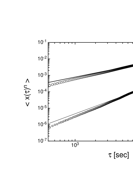
Figure 12: The moments $\left<x^{n}(\tau)\right>$ of the price increment $x(\tau)$ as functions of the time scale $\tau$ for order $n=2$ (top) and $n=4$ (bottom). Throughout the range $\tau_{min}\;\leq\;\tau\;\leq 12h$ the moments are in good approximation described by power laws (straight lines).

Using the results for the second and fourth order moments, equations (22) can easily be solved and yield estimates for the unkown functions $\alpha(\tau)$ and $\beta(\tau)$. We find that $\alpha$ is a linear function of the time scale $\tau$ with a slope $\alpha_{0}$ of $0.016d^{-1}$, while $\beta$ is approximately constant in $\tau$ and has a value of $0.11$. Let us summarize our results for $D_{1}$ and $D_{2}$:

$$D_{1}(x,\tau)\; = \;-\,\gamma\,x$$

$$\gamma\; = \;0.93\,\pm\,0.02$$

$$D_{2}(x,\tau)\; = \;\alpha_{0}\,\tau\;+\;\beta\,x^{2}$$

$$\alpha_{0}\; = \;0.016d^{-1}\,\pm\,0.002d^{-1}$$

$$\beta(\tau)\; \approx \;const\;=\;0.11\,\pm\,0.02.$$ (25)

3.6 Consistency Checks

The results and assumptions of the preceeding sections lead to Fokker- Planck equations for the pdf $p(x,\tau)$ and the conditional pdf $p(x,\tau|x_{0},\tau_{0})$, respectively (equations (10) and (9)). The coefficients $D_{1}$ and $D_{2}$ which completely determine these equations were estimated from the data. Thus we can claim to have found the complete description of the stochastic process for the data. In order to test this result, we compare the (numerical) solution of the Fokker-Planck equation with the distributions obtained directly from the data. The algorithm used for the numerical iteration is based on the approximative solution of the Fokker-Planck equation for small steps $\Delta\tau$. According to [14], the conditional pdf $p(x_{1},\tau_{0}-\Delta\tau|x_{0},\tau_{0})$ is, for small $\Delta\tau$ and arbitrary $D_{1}$ and $D_{2}$, a Gaussian distribution in $x_{1}$ with mean value $x_{0}-D_{1}\Delta\tau$ and standard deviation $\sqrt{2D_{2}\Delta\tau}$. In order to obtain the conditional densities for larger steps, we use the Chapman-Kolmogorov equation

$$p(x_{2},\tau_{0}-2\Delta\tau|x_{0},\tau_{0})=\int\limits_{-\infty}^{+\infty}p(x_{2},\tau_{0}-2\Delta\tau|x_{1},\tau_{0}-\Delta\tau)p(x_{1},\tau_{0}-\Delta\tau|x_{0},\tau_{0})dx_{1}.$$ (26)

(26) is a direct consequence of the Markov condition (4). Iterating this procedure, we finally obtain the conditional pdf $p(x,\tau_{0}-n\Delta\tau|x_{0},\tau_{0})$. Multiplying with $p(x_{0},\tau_{0})$ and integrating with respect to $x_{0}$ yields the pdf $p(x,\tau_{0}-n\Delta\tau)$.

Figure 13, which compares the solutions of the Fokker-Planck equation for the pdf $p(x,\tau)$ with the empirically estimated pdfs, proves that the Fokker-Planck equation accurately describes the evolution of $p(x,\tau)$ in $\tau$ over the range $4min\leq\tau\leq 12h$.

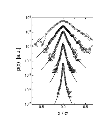
Figure 13: Comparison of the numerical solutions of the Fokker-Planck equation (solid lines) for the pdfs $p(x,\tau)$ with the pdfs obtained directly from the data (open symbols). The scales $\tau$ are (from top to bottom): $\tau\;=\;12h,\,4h,\,1h,\,15min$ and $4min$. The pdf at the largest scale $\tau=12h$ was parametrized (dashed line) and used as inital condition for the iteration of the Fokker-Planck equation. Curves are shifted in vertical direction for clarity of presentation.

As mentioned above, the Fokker-Planck equation also governs the conditional pdf $p(x,\tau|x_{0},\tau_{0})$. As a further test of our results, we calculated the solutions of the Fokker-Planck equation (9). Figure 14 shows the result for $\tau_{0}=1h$ and $\tau=0.5h$, again in comparison with empirical data. Taking into account the various uncertainties and assumptions in the determination of the coefficients $D_{1}$ and $D_{2}$, the agreement between the solution of (9) and the data is remarkably good.

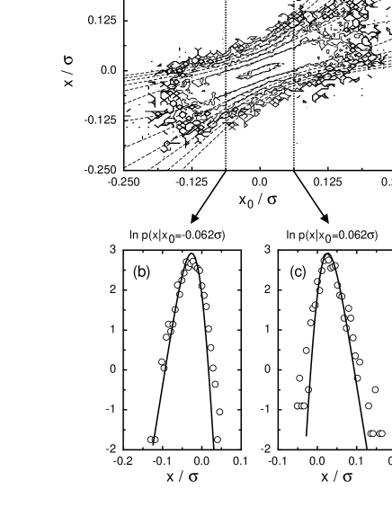
Figure 14: Comparison of the numerical solution of the Fokker-Planck equation for the conditional pdf $p(x,\tau|x_{0},\tau_{0})$ with the emprical data.
(a): Contour plots of $p(x,\tau|x_{0},\tau_{0})$ for $\tau_{0}=1h$ and $\tau=0.5h$. Dashed lines: numerical solution of eq. (9), solid lines: empricial data.
(b) and (c): Cuts through $p(x,\tau|x_{0},\tau_{0})$ for $x_{0}=-0.062\sigma$ and $x_{0}=+0.062\sigma$, respectively. Open symbols: empirical data, solid lines: numerical solution of the Fokker-Planck equation.

4 Summary and Conclusions

The purpose of the present article is to show how the mathematical framework of Markov processes can be applied to the analysis of emprical high frequency exchange rate data. Within the limitations due to the finite number of samples, we were able to verify the Markovian properties of the price increment for time delays $\tau$ larger than $\tau_{min}=4min$.

Furthermore, we obtained estimates for the Kramers-Moyal coefficients $D_{k}(x,\tau)$ and found hints that the fourth order coefficient $D_{4}$ is zero. The comparison of the solutions of the resulting Fokker- Planck equations with the empricial distributions strongly supports our results for $D_{1}$ and $D_{2}$.

It is worth to note that the results given in the present article differ from the results of our previous analysis presented in [12]. While in [12] $D_{1}$ and $D_{2}$ were also found to be linear and quadratic functions of $x$, respectively, the values given for the coefficients $\gamma$, $\alpha$ and $\beta$ were different from the ones given here in equation (25).

The analysis presented in [12] is incomplete, because it did not take into account the presence of the additive white noise (see section 3.1) and mainly focused on the functional dependence of the $D_{k}$ on $x$. The numerical values of the coefficients $\gamma$, $\alpha$ and $\beta$ were chosen such that the pdfs of the price increment $x$ were fitted best by the resulting Fokker-Planck equation. However, it can be shown that the coefficients given in [12] fail to describe the conditional pdf $p(x,\tau|x_{0},\tau_{0})$, i.e. cannot be correct.

This is a quite important result: There are several choices for the coefficients which correctly describe the one-point distribution $p(x,\tau)$, but only one choice which also describes the joint statistical properties of several increments on different scales. This, in turn, means that a complete statistical characterization of the price increments (or returns) necessarily has to include the multi-scale statistics and must not be restricted to the analysis of increments (or returns) on only one scale.

The results of our analysis presented in this paper also eliminate the discrepancy between our approach as presented in [12] and the often reported power-law behaviour of the distributions of returns. As previously shown in [17], the solutions of the Fokker-Planck equation asymptotically show scaling behaviour with a scaling exponent $\mu$ which can be calculated from the linear and quadratic coefficient of $D_{1}$ and $D_{2}$, respectively:

$$\mu\;=\;\frac{\gamma}{2\,\beta}.$$ (27)

While the values reported in [12] lead to a value of about $12$ for the scaling exponent $\mu$, in disagreement with the usually observed value between 3 and 5, our new values (25) yield $\mu\,=\,4.2\pm 0.8$.

Another interesting result of our analysis concerns the symmetry of the stochastic process underlying the evolution of the price increment $x$ in the scale variable $\tau$. According to (25), the drift coefficient $D_{1}$ is completely antisymmetric in $x$ ($D_{1}(-x)\,=\,-D_{1}(x)$), while the diffusion coefficient $D_{2}$ is symmetric in $x$. The resulting Fokker-Planck equation (10) for the pdf $p(x,\tau)$ is symmetric in $x$. This means that if the large scale pdf, which serves as the initial condition for the partial differential equation (10), was symmetric, it would remain symmetric for all scales $\tau$. In other words: The asymmetries of the distributions of price increments on small scales are solely due to the asymmetry of the increment at the largest scale, i.e. they are a consequence of some market event on long terms. The stochastic process itself, at least on scales smaller than a day, is symmetric in $x$. This result might provide a possibility to distinct between trends (as for example caused by the long term development of a country’s economy) and the short term fluctuations caused by the market itself i.e. by the interactions of several agents trading an asset. This fits well with the results of commonly discussed market models, which are quite succesfull in qualitatively explaining most of the features of real markets but which do not naturally exhibit asymmetries between positive and negative returns, see for example [18] and [19]. Our result indicates that there is no need to incorporate asymmetries in such models. However, so far we can only present results for a single data set over an one-year period. Further studies on a larger variety of assets and time scales will be necessary to check the significance of this particular result.

Finally, we would like to comment on the proposed analogy between financial markets and turbulent hydrodynamic flows, cf. [20]. The complex statistical behaviour of velocity increments on a certain length scale in turbulent flows is assumed to be due to a cascading process. Energy, which is fed into the system on large scales, is continuously transported towards smaller scales due to the inherent instability of vortices of a given scale towards perturbations on smaller scales. Finally, the energy is dissipated at the smallest scale.

A similar mechanism has been proposed for financial markets, where the energy cascade was replaced by a flow of information. Initially, the assumption of a cascading process in financial markets was based on similarities in the empirical description of the pdfs of price and velocity increments, respectively [20]. The analogy between turbulence and finance has inspired many further studies (see, for example, [21], [22], [23]), but has also been criticized for being too superficial [9].

However, the results of the Markov analysis of financial and turbulent data (see [16] for details on the Markov analysis of turbulence) allow for a more detailed comparison of the stochastic processes underlying the two phenomena with the predictions of common cascade models.

The most prominent model for turbulence is Kolmogorov’s theory dating back to 1962 (furtheron refered to as K62). The prediction of the K62 model for the coefficients $D_{1}$ and $D_{2}$ can easily be shown to be [24]:

$$D_{1} \;=\; -\,\gamma\,x,$$

$$D_{2} \;=\; \beta\,x^{2},$$ (28)

where $\gamma$ and $\beta$ both are constant ($\gamma\approx 1/3$ for turbulence). Castaing [25] proposed the model of a multiplicative cascade where the increment on a given scale is linked to an increment at a larger scale via a random multiplier. This model was shown to imply Markovian properties [26] and to predict coefficients $D_{1}$ and $D_{2}$ similar to those predicted by K62, except that it allows for a scale dependence of $\gamma$ and $\beta$.

Recently, Dubrulle [27] proposed an extension of Castaing’s multiplicative cascade model which incorporates additive noise. Comparing the results (25) of our analysis with the predictions of the various models, we can state that the statistics of the price increment is well described by the model of a multiplicative cascade with additive noise (or, in the notion of [17], by the mechanism of ”multiplicative noise with reinjection”).

It is interesting to note the result of the Markov analysis for fully developed turbulent flows [16]. It turns out that measured turbulent data are not completely described by any of the above mentioned models. While $D_{1}$ turns out to be linear, $D_{2}$ exhibits are more complicated dependence on the increment than predicted by the multiplicative cascade models. In particular, we find a linear term in $D_{2}$ which breaks the symmetry and which is by no means negligable, see [16]. In some sense, one might therefore say that financial data are much closer to ideal ”Kolmogorov-like” turbulence than turbulent data. Besides this analogy we found a clear differene in the mechanisms leading to the finite step-size of the cascade processes. In the case of turbulence a smoothing out due to viscosty was found, while financial markets seem to be dominated by some uncoorelated additional noise on the smallest scales.

Summarizing, it is the concept of a cascade in time hierarchy that allowed us to derive the results of the present paper, which in turn quantitatively supports the initial concept of an analogy between turbulence and financial data. Furthermore, we have shown that the smooth evolution of the pdfs down along the cascade towards smaller time delays is caused by a Markov process with multiplicative noise.

Metaphorically, our characterization of volatility of currency markets as random and uneven flow of information to the markets is similar to [7] which describes stochastic process of the stochastic volatility model as random and uneven flow of news to the financial markets.

References

- [1] L. Bachelier, Theorie de la speculation, Ph.D. Thesis, Annales Scientifiques de l’Ecole Normal Superieure III-17, 1900.
- [2] Engel, R. F. and M. Rothschild, (eds.). (1992). Journal of Econometrics, A supplement to the Journal of Econometrics, Vol. 52.
- [3] Bollerslev, T., 1986. Generalized autoregressive conditional heteroskedasticity. Journal of Econometrics. 31, 307-327.
- [4] Bollerslev, T., Chou, R. Y., Kroner, K.F., 1992. ARCH modeling in finance: a review of the theory and empirical evidence. Journal of Economterics, 52, 5–59.
- [5] Taylor, S. J., 1994. Modelling stochastic volatility: a review and comparative study. Mathematical Finance, 4, 183–204.
- [6] Ghysels, E., Harvey, A., and Renault, E. (1996). Stochastic Volatility. In: Handbook of Statistics (vol. 14), eds. G. S. Maddala and C.R. Rao, Amsterdam: North-Holland, pp. 119-191.
- [7] Gallant, A. R., Hsieh, D., Tauchen, G., Estimation of stochastic volatility models with diagnostics. Journal of Econometrics, 81, 159–192.
- [8] R. Mantegna & H.E. Stanley 1996. Turbulence and financial markets. Nature 383, 767.
- [9] R. Mantegna & H.E. Stanley 1999. An introduction to econophysics. Cambridge University Press, Cambridge.
- [10] H.E Stanley et al., Quantifying fluctuations in economic systems by adapting methods of statistical physics, Physica A 287 (2000) 339 - 361.
- [11] Voit, J., The Statistical Mechanics of Financial Markets. Springer-Verlag, Heidelberg (2001).
- [12] Friedrich, R., Peinke, J. and Renner, Ch. (2000). How to quantify deterministic and random influences on the statistics of the foreign exchange market. Phys. Rev. Lett., 84, 5224–5227.
- [13] Heald, J.P.M. and Stark, J. (2000) Estimation of Noise Levels for Models of Chaotic Dynamical Systems. Phys. Rev. Lett., 84, 2366–2369
- [14] Risken, H., The Fokker-Planck equation, (Springer-Verlag Berlin, 1984); Van Kampen,N. G., Stochastic processes in physics and chemistry (North Holland, Amsterdam, 1981); Gardiner, C.W. Handbook of Stochastic Methods, (Springer-Verlag Berlin, 1983)
- [15] Hänggi, P. & Thomas, H. 1982 Stochastic processes: Time evolution, symmetries and linear response Physics Reports 88, 207.
- [16] Rener, Ch., Peinke, J. and Friedrich, R. Experimental indications for Markov properties of small scale turbulence. JFM 433 (2001), 383-409.
- [17] D. Sornette, Fokker-Planck equation of distributions of financial returns and power laws. Physica A 290 (2001) 211–217.
- [18] R. Cont, J.P. Bouchaud, Herd behaviour and aggregate fluctuations in finacial markets. cond-mat/9712318.
- [19] D. Stauffer, D. Sornette, Self-organized percolation model for stock market fluctuations, Physica A 271 (1999) 496–506.
- [20] Ghashghaie, S., Breymann, W., Peinke, J., Talkner, P., Dodge, Y., 1996. Turbulent cascade in foreign exchange markets. Nature 381, 767–770.
- [21] A. Arneodo, J.-F. Muzy & D. Sornette, ”Direct” causal cascade in the stock market. Eur. Phys. J. B 2 (1998), 277–282.
- [22] F. Schmitt, D. Schertzer & S. Lovejoy, Multifractal analysis of foreign exchange data. Appl. Stoch. Model D. A. 15 (1), 1999.
- [23] W. Breymann, S. Gashghaie & P. Talkner, A stochastic cascade model for FX dynamics. International journal of theoretical and applied finance (IJTAf) 3 (3), 357–360, 2000.
- [24] Friedrich, R., Peinke, J., Physica D 102, 147 (1997); Friedrich, R., Peinke, J., Phys. Rev. Lett. 78, 863 (1997)
- [25] B. Castaing, Y. Gagne & E.J. Hopfinger, Physica D 46, 177–200 (1990); B. Castaing, J. Phys. II France 6 105 (1996).
- [26] P.-O. Amblard & J.-M. Brossier, On the cascade in fully developed turbulence. The propagator approach versus the Markovian description. Eur. Phys. J. B 12 (1999), 579–582.
- [27] B. Dubrulle, Affine turbulence. Eur. Phys. J. B 13, 1 (2000).